Суперкомпьютерные дни в России 2016 // Russian Supercomputing Days 2016 // RussianSCDays.org
A parallel algorithm for 3D modeling of monochromatic acoustic field by the method of integral equations ∗ M.S. Malovichko1, N.I. Khokhlov1, N.B. Yavich1, M.S. Zhdanov2 Moscow Institute of Physics and Technology1, The University of Utah2 We present a parallel algorithm for solution of the three-dimensional Helmholtz equation in the frequency domain by the method of volume integral equations. The algorithm is applied to seismic forward modeling. The method of integral equations reduces the size of the problem by dividing the geologic model into the anomalous and background parts, but leads to a dense system matrix. A tolerable memory consumption and numerical complexity were achieved by applying an iterative solver, accompanied by an effective matrix-vector multiplication operation, based on the fast Fourier transform. We used OpenMP to speed up the matrix-vector multiplication, while MPI was used to speed up the equation system solver, and also for parallelizing across multiple sources. Practical examples and efficiency tests are presented. Keywords: Fredholm integral equations, acoustics, seismics, MPI, OpenMP.
1. Introduction The method of integral equations (IE) is a well-known wavefield modeling technique [2,9]. It has a number of attractive properties. It requires discretization for the anomalous volume only. It drastically reduces the size of a problem in many applications. The IE formulation does not require boundary conditions. It also can be naturally used to compute the Fr´echet derivatives and for this reason it is very attractive for inverse problems. The IE method is based on the discretization of the original integral equation and results in a complex-valued dense matrix. In a straightforward implementation, the computational burden becomes prohibitive for large three-dimensional problems, encountered in seismology. Yet some studies, many of them for the two-dimensional solution, have been reported [4–6,8,11]. Recently, the full method of IE, accompanied with an iterative solver, was applied to the visco-acoustic three-dimensional modeling [1]. The authors of [1] have implemented Green’s integral operator for the free space background model via the Fourier transform (this idea itself is quite old). An effective matrix-free implementation allowed them application of the BiCGStab method to resulting system of linear equations with the cost per iteration of O(N logN ), where N is the number of model cells. They showed, that a realistically large acoustic model can be simulated almost as effectively with the IE method, as it is for finite-different schemes. In this study, we design a parallel version of the solver for the half-space host medium, and study the efficiency of parallelization.
2. Problem formulation We consider a 3D model consisting of a half-space host medium and an anomalous volume D, confined within the lower half-space. The host medium has piece-wise constant density and acoustic velocity: ρ0 and c0 for the upper half-space; ρb and cb for the lower half space. The anomalous volume has the same background density ρb , and arbitrary distribution of velocity c = c(r), where r is the position vector. Let ω be the circular frequency. Assuming a lossless medium, we define the anomalous velocity ca = c − cb , wavenumber k = ω/c, background wavenumber kb = ω/cb and parameter χ = 1/c2 − 1/c2b . The pressure response p to a point ∗
This research was supported by the Russian Science Foundation, project No. 16-11-10188.
4
Суперкомпьютерные дни в России 2016 // Russian Supercomputing Days 2016 // RussianSCDays.org
source at a given frequency ω satisfies to the following Lippmann-Schwinger equation: p − G[ω 2 χp] = pb , where pb is the background field, G is the integral operator, defined for any scalar field f , Z G[f ] = g(r|r0 )f (r0 )dV 0 ,
(1)
(2)
D
where g is the background Green’s function. Let the anomalous volume be covered by N = Nx Ny Nz cubical cells. After discretization we receive the following matrix equation: Au = b,
(3)
where u = (p1 ..pN ) is the vector of N unknown values approximating p in the center of each cell, b = (pb,1 ..pb,N ) is known values of the background field in each cell, A is the scattering matrix, A = (I − GX),
(4)
where I is the identity matrix, X = diag(χ1 ..χN ) is a diagonal matrix formed by contrasts for each cell, G contains integrals of Green’s function over cells, Z g(rm |r0 )dV 0 , m, n = 1..N. (5) Gmn = Dn
Matrix A is a dense complex-valued non-hermitian matrix with real-valued spectrum. Its condition number substantially improves at lower frequencies since in this case matrix spectrum has a weak dependence on the grid step size and velocity model. These properties make the IE equation system more attractive for iterative solution than that of the finite-difference method. To solve system (3) we use the unpreconditioned BiCGStab iterative solver [10]. An effective implementation of the matrix-vector multiplication is critical for iterative solutions. In case of a layered background medium Green’s function g has lateral symmetry, i.e. g(r|r0 ) = g(x − x0 , y − y 0 , z, z 0 ). Thus, for interior points (r ∈ D), Ny Nx Nz X X X Inml = G(xn − xi , ym − yj , zl , zk )f (xi , yj , zk ), k=1
(6)
(7)
j=1 i=1
where Inml is the value of G[f ] for a cell located at (xn , ym , zl ). The expression inside the outer parenthesis is essentially a 2D convolution for given k and l. Being implemented with 2D FFT, it takes O(Nx Ny log(Nx Ny )). This should be performed Nz2 times (for every k-l combination). Finally, the total complexity for matrix-vector multiplication in the case of a layered host model is O(N Nz log(Nx Ny )). The memory requirements is O(N Nz ), though this amount can be reduced to O(N ) at the expense of increased running time if the values of G are calculated on-the-fly.
3. Parallelization Our code exploits three levels of parallelism: parallel execution of the matrix-vector product, parallel system solution, and data decomposition across multiple acoustic sources (Figure 1). The BiCGStab solver requires four inner products and two matrix-vector products per iteration. The inner products are easily parallelized, though in distributed-memory systems some
5
Суперкомпьютерные дни в России 2016 // Russian Supercomputing Days 2016 // RussianSCDays.org
Figure 1: Layers of parallelism on a hybrid cluster.
collective communication is required. In this study we have used the standard MPI collective communication routines. This overhead is negligible for our typical tasks. The matrix-vector multiplications are easily parallelized within a single computational node with OpenMP. On a distributed-memory system, this operation becomes the most problematic part, because each model cell is connected with all other cells through the integral operator. No matter what the distribution scheme is selected (splitting the matrix into strips across MPI processes with subsequent assembling the resulting vector on a single MPI process, or splitting the matrix into vertical strips and subsequent reduction of resulting vectors on a single MPI process), when the matrix-vector product is computed, it must be sent to all other MPI processes for they update their copies. It can be expected, that this level scales to O(logP ), where P is the number of processes, that communicate during the system solutions [7]. This may create huge network traffic for large P . The highest level of parallelism is the distribution of different seismic sources across several MPI groups. In our tasks a forward problem typically has to be solved for many sources (several thousand) for the same model. Naturally, the available pool of MPI processes is divided into several groups. All processes in a group have their copies of model parameters and simultaneously work on a subset of sources, processing them one by one.
4. Numerical tests In this section we present the results of numerical experiments. We used two types of hardware. All tests, involving several computing nodes, such as those shown in Figure 2a and Figure 2b (labels ”Type 1”), have been performed on a hybrid cluster. Each node consisted of twelve-core Intel Xeon (Westmere X5660) processors running at 2.8GHz and was equipped with 24Gb RAM and QDR Infiniband interconnect. All tests on a shared-memory system (Figure 2b, labels ”Type 2”, and Figure 2c) have been performed on a workstation with a single twelve-core Intel Xeon E5-2620 processor running at 2.10GHz. The highest level of parallelism, i.e. the distribution of seismic sources across different MPI groups, should scale almost linearly in K, where K is the number of equally-sized MPI groups. In our tests, which involved a moderate number of nodes, the overhead can be neglected. For the first test we selected a model with 2’097’152 cells (128 cells in each direction). There were 32 seismic sources, located at the surface. The size of a single MPI group was constant and set to unity. We ran computations with 1, 4, 8, 16, and 32 nodes, i.e. each node had to solve 32, 8, 4, 2, and 1 forward problems, respectively. The resulting speedup (Figure 2a) confirmed, that the task decomposition has produced a good acceleration. In the next test, only one forward problem (a single source) has been solved. The iterative solver ran in parallel on varying number of MPI processes. The curve labeled ”Type 1” (Figure 2b) has been obtained on a cluster, on which one MPI process was running on a single node with 12 cores. The curves, named ”Type 2”, have been obtained on a single 12-core node,
6
Суперкомпьютерные дни в России 2016 // Russian Supercomputing Days 2016 // RussianSCDays.org
(a)
(b)
(c)
Figure 2: Scalability tests. (a) - distribution of sources across MPI groups, (b) - system solution with several MPI processes, (c) - matrix-vector parallelization with OpenMP threads.
where each core was running an MPI process. For this test we used four different models, in which the number of cells was varying from 40’960 cells to 2’097’152 cells (see the plot legend). The speedup rapidly deteriorates as the number of processes per system grows. For the largest model, the computational time dominates the communication time until 16 process per system. For smaller models the speedup began to deteriorate at lower K. In the third test, we studied the performance of the matrix-vector multiplication leveraged with the shared-memory parallelization. There were three runs with three models of different sizes (Figure 2c). The resulting speedup curves revealed fairly good scaling versus the number of cores. The speedup for the smallest model suffered from the fact, that the background field pb was computed on the master thread. However, for the larger models, where the matrix-vector operations dominated, the efficiency was above 86%.
5. Conclusion We have designed a parallel solver for 3D frequency-domain modeling of the acoustic field. The equation system is solved iteratively; the matrix-vector product is performed via FFT. It makes the computational complexity and memory requirements tolerable for realistically large problems. We have extended this approach by parallelizing the code at three levels: the distribution of seismic sources across different groups of MPI processes, solution of the equation system with several MPI processes, and parallelization of the matrix-vector multiplication over OpenMP threads. We have studied the efficiency of all three levels of parallelism. The parallelization of the system solution has been found be the most difficult part, because the system matrix is dense. This limited the speedup of this level. Presumably, any algorithms, based on the volume integral equations, would have similar problems. On the other hand, the coarse-grained (the distribution of sources) and fine-grained parallelism (matrix-vector product) have a good scalability. We expect, that the presented approach might be quite effective on CPU-GPU clusters, especially in case of multi-frequency and multi-source simulation, which are often encountered in seismic applications. The presented results confirm, that the integral-equation modeling can be applied to realistic problems, and is quite promising for seismic applications involving multiple sources/frequencies.
References 1. Abubakar, A., T.M. Habashy. Three-dimensional visco-acoustic modeling using a renormalized integral equation iterative solver. //Journal of computational physics, vol. 249, pp.1-12, 2013.
7
Суперкомпьютерные дни в России 2016 // Russian Supercomputing Days 2016 // RussianSCDays.org
2. Aki, K. and P. G. Richards. Quantitative seismology. 1980. W. R. Freeman and Co. 3. Aminzadeh, F., Brac, J., Kunz, T. 3-D Salt and Overthrust Models. SEG/EAGE 3-D Modeling Series No.1., Soc. Explor. Geophysicists, Tulsa, 1997. 4. Freter, H. An Integral Equation Method for Seismic Modelling// in Inversion Theory and Practice of Geophysical Data Inversion, vol. 5, 1992. Vieweg+Teubner Verlag. 5. Fu, Li-Yun. Numerical study of generalized Lippmann-Schwinger integral equation including surface topography. //Geophysics, vol. 68, no. 2, pp.665-671, 2003. 6. Fu, Li-Yun, Yong-Guang Mu, Huey-Ju Yang. Forward problem of nonlinear Fredholm integral equation in reference medium via velocity-weighted wavefield function. //Geophysics, vol. 62, no. 2, pp.650-656, 1997. 7. Grama, A., A. Gupta, G. Karypis, V. Kumar Introduction to parallel computing, 2nd ed. Addison Wesley, 2003. 8. Johnson, S.A., Y. Zhou, M.J. Berggren, M.L. Tracy. Acoustic Inverse Scattering Solutions by Moment Methods and Back Propagation // Conference on inverse scattering: theory and applications. 1983. SIAM. 9. Morse, P. M. and Feshbach, H. Methods in theoretical physics. 1953, McGraw-Hill Book Company, inc. 10. Saad, Y. Iterative methods for sparse linear systems, 2nd ed., SIAM, Philadelphia, PA, USA. 2003. 11. Zhang, Rongfeng , Tadeusz J. Ulrych. Seismic forward modeling by integral equation and some practical considerations. //SEG Technical Program Expanded Abstracts 2000, chp. 593, pp. 2329-2332, SEG, 2000.
8