6.3 Velocity distribution, bed roughness and friction factors in unvegetated channels
6.3.1 Viscous sublayer
On the bottom of an unvegetated channel there is no turbulence and the turbulent shear stress τt =0, and therefore in a very thin layer above the bottom, viscous stress is dominant, and hence flow is laminar in that layer called viscous sublayer.
Above the viscous sublayer the turbulent stress dominates and the total stress can be calculated from Eq. (6-16), i.e. as the sum of viscous and turbulent shear stresses.
τ z = τ v + τ t = ρg( h − z )So
(6-16)
The total stress decreases linearly towards zero when approaching the water surface (z approaches water depth h). The distribution of the shear stress as a function of z is completely analogous with the hydrostatic pressure p=ρg(h-z) with the exception of the viscous sublayer close to the bottom.
6.3.2 Scientific classification of flow layers in unvegetated channels
According to Liu (2001) the so called scientific classification of flow layers is the one shown in Fig. 6-4.
Last update September 2009. Original material by Tuomo Karvonen, 2002. Department of Civil and Environmental Engineering, Helsinki University of Technology. http://civil.tkk.fi/fi/tutkimus/vesitalous/www_oppikirjat/yhd_122010/
75
Fig. 6-4. Scientific classification of flow regions in unvegetated channels (not to scale). Adapted from Liu (2001).
Near the bottom there is the thin viscous sublayer where there is almost no turbulence. Measurements show that the viscous shear stress in this layer is constant and equal to the bottom shear stress τb. Flow in this layer is laminar. In the transition layer viscosity and turbulence are equally important. In the turbulent logarithmic layer viscous shear stress is negligible and the turbulent shear stress is equal to the bottom shear stress. The Prandtl's mixing length theory was developed for this layer and it leads to the logarithmic velocity profile as shown later on. The turbulent outer region consists of about 80-90 % of the total region and velocity is relatively constant due to the strong mixing of the flow (Liu 2001).
6.3.3 Bed roughness ks in unvegetated channels
Bed roughness ks is very often also called roughness height (karkeuskorkeus in Finnish) or equivalent roughness (ekvivalentti karkeus).
One important question is how to determine the bed roughness ks. Nikuradse made his experiments by glueing grains of uniform size to pipe surfaces. In completely flat bed consisted of uniform spheres the bed roughness ks would be the diameter of the grains.
Last update September 2009. Original material by Tuomo Karvonen, 2002. Department of Civil and Environmental Engineering, Helsinki University of Technology. http://civil.tkk.fi/fi/tutkimus/vesitalous/www_oppikirjat/yhd_122010/
76
This cannot be found in nature, where the bed material is composed of grains with different size and bottom itself is not flat but it includes ripples or dunes (see Fig. 6-5).
According to Liu (2001), the following ks values have been suggested based on different type of experiments: • concrete bottom
ks=0.001 - 0.01 m
• flat sand bed
ks= (1 - 10)d50
• bed with sand ripples ks=(0.5 - 1.0)Hr : Hr = ripple height (m)
Fig. 6-5. Ripples and dunes (adapted from Liu 2001).
6.3.4 Characterisation of smooth and rough flow in unvegetated channel
It is necessary to characterise the flow as hydraulically smooth or rough since it influences e.g. the thickness of the viscous sublayer etc. A very big series of experiments were carried out by Nikuradse for pipe flows. He introduced the concept of equivalent grain roughness ks, which is usually called bed roughness for open channel flow. Based on the experiments it was found that the following criteria can be used to characterise if flow is hydraulically smooth, rough or in the transitional zone:
Last update September 2009. Original material by Tuomo Karvonen, 2002. Department of Civil and Environmental Engineering, Helsinki University of Technology. http://civil.tkk.fi/fi/tutkimus/vesitalous/www_oppikirjat/yhd_122010/
77
v *k s ≤ 5; hydraulica lly smooth flow ν v *k s ≥ 70; hydraulica lly rough flow ν v k 5 ≤ * s ≤ 70; hydraulica lly transition al flow ν
(6-18)
where v* is the friction velocity calculated using Eq. (6-15) and ν is the kinematic viscosity.
6.3.5 Logarithmic velocity distribution in turbulent layer
It was described in section 6.3.2 that the measurements show that the turbulent shear stress is constant in the turbulent logarithmic layer and it equals the bottom shear stress. By assuming that the mixing length is proportional to the distance to the bottom, lm=κz (κ is von Karman constant), Prandtl obtained the logarithmic velocity profile. By the modifications done to the original theory, the logarithmic velocity profile applies also in the transitional layer and in the turbulent outer layer. Measured and computed velocities show reasonable agreement. This means that from an engineering point of view, two different velocity profiles need to be considered (Liu 2001): • logarithmic velocity distribution, which covers the transition layer, turbulent logarithmic layer and turbulent outer layer from Fig. 6-4. • velocity profile in the viscous sublayer
In the turbulent layer the total shear stress is assumed to contain only the turbulent shear stress. The total shear stress increases linearly with depth
z τ t (z ) = τ b (1 − ) h
(6-19)
According to Prandtl's mixing length theory shown in section 6.2.2 and Eq. (6-6)
dv τ t = ρl 2m
2
(6-6)
dz
Last update September 2009. Original material by Tuomo Karvonen, 2002. Department of Civil and Environmental Engineering, Helsinki University of Technology. http://civil.tkk.fi/fi/tutkimus/vesitalous/www_oppikirjat/yhd_122010/
78
Now comes out the modification of the original theory. Instead of assuming that the mixing length lm=κz like Prandtl assumed, lm is replaced by equation
z l m = κz (1 − )0.5 h
(6-20)
It is possible to combine (6-20) and (6-6) to get
dv = dz
τb / ρ v * = κz κz
(6-21)
Eq. (6-21) can be integrated from z0 to h to get the logarithmic velocity profile.
v z v (z ) = * ln κ z0
(6-22a)
The integration constant z0 is the elevation corresponding to zero velocity (see Fig. 6-6).
Note: Most often the "universal" logarithmic velocity distribution is shown in the form:
v( z) 1 z = ln + 8.5 κ ks v*
(6-22b)
See next page for comparison of (6-22a) and (6-22b)!
Note the similarity to the calculation of aerodynamic resistance ra needed in the estimation of potential evapotranspiration rate using the Penman-Monteith equation! In these calculations the roughness length is usually around 10-13 % of the crop height!
Last update September 2009. Original material by Tuomo Karvonen, 2002. Department of Civil and Environmental Engineering, Helsinki University of Technology. http://civil.tkk.fi/fi/tutkimus/vesitalous/www_oppikirjat/yhd_122010/
79
Fig. 6-6. Velocity distribution in hydraulically smooth and rough flow (graphs not to scale).
The integration constant z0 (m) is here based on the study conducted by Nikuradse for pipe flows.
ν 0 . 11 v* z 0 = 0.033k s ν 0 . 11 + 0.033k s v *
v *k s ≤ 5; hydraulica lly smooth flow ν v *k s (6-23) ≥ 70; hydraulica lly rough flow ν v k 5 ≤ * s ≤ 70; hydraulica lly transition al flow ν
NOTE! Eqs. (6-22a) and (6-22b) are exactly the same since (6-22b) is valid from z-values which give v(z) greater than or equal to zero. v(z) given by (6-22b) is zero when
z ( v = 0) = k se −8.5κ = 0.033k s = z 0
(for rough flow )
(6-22c)
The friction velocity v* is the fluid velocity very close to the bottom and it is the flow velocity at elevation z=z0eκ, i.e.
v
z = z 0e κ
= v*
Last update September 2009. Original material by Tuomo Karvonen, 2002. Department of Civil and Environmental Engineering, Helsinki University of Technology. http://civil.tkk.fi/fi/tutkimus/vesitalous/www_oppikirjat/yhd_122010/
(6-24)
80
6.3.6 Velocity profile in the viscous sublayer
In the case of hydraulically smooth flow there is a viscous sublayer whereas in the rough flow there is a height z0 with zero flow (Figs. 6-6 and 6-7). Viscous shear stress is constant in the viscous sublayer and it is equal to the bottom shear stress as shown in Fig. 6-4.
τν = ρν
dv = τb dz
(6-25)
Eq. (6-25) can be integrated assuming that velocity v=0 when z=0. Integration gives
τb ρ v (z ) = z= ν
v *2 z ν
(6-26)
giving a linear velocity distribution in the viscous sublayer. The thickness of the viscous sublayer can be obtained by finding the z value where the logarithmic velocity distribution intersects the linear distribution giving a theoretical thickness of the viscous sublayer δν (Liu 2001).
δ ν = 11.6
ν v*
(6-27)
Summary of the velocity profiles in the hydraulically smooth and rough flow is given in Fig. 6-7.
Last update September 2009. Original material by Tuomo Karvonen, 2002. Department of Civil and Environmental Engineering, Helsinki University of Technology. http://civil.tkk.fi/fi/tutkimus/vesitalous/www_oppikirjat/yhd_122010/
81
Fig. 6-7. Summary of the velocity profiles in hydraulically smooth and hydraulically rough flow (in the graph u(z) refers to v(z) and u* refers v*).
6.3.7 Drag force
Flowing water moving past an object will exert a force called drag force
1 FD = ρC D Av 2 2
(6-28)
where CD is the coefficient and A is the projected area of the object to the flow direction. Values of CD are usually around 1.0...2.0 but experiments are needed for more accurate determination of the values. Drag force comes partly from the skin friction when water moves around the object and partly from the pressure the moving water exerts on the object.
Correspondingly to the drag force another force called lift force FL can be defined. It has the same shape than the drag force:
1 FL = ρC L Av 2 2
(6-29)
where CL is the lift coefficient which also need to be determined experimentally.
Last update September 2009. Original material by Tuomo Karvonen, 2002. Department of Civil and Environmental Engineering, Helsinki University of Technology. http://civil.tkk.fi/fi/tutkimus/vesitalous/www_oppikirjat/yhd_122010/
82
6.3.8 Chézy, Manning and Darcy-Weissbach friction coefficients
The three most often used equation for calculating friction losses hf (Eqs. 6-30) are the ones known as Chézy, Manning and Darcy-Weissbach equations.
1 Lv 2 hf = C2 R 2 2 Lv hf = n 4/3
Chézy Manning
(6-30)
R
L v2 h f = f DW 4R 2g
Darcy − Weissbach
where L is the length of the river section and R is hydraulic radius. C is the Chézy coefficient, n =1/kSt is the Manning coefficient (the inverse of n is kSt called the Strickler coefficient) and fWD is the Darcy-Weissbach friction coefficient originally developed for pipe flow. Note the hf is linearly related to fWD but to C2 and n2.
There is the following connection between the different friction coefficients:
f DW = 8gR −1 / 3n 2 = 8gC − 2
(6-31)
The three different friction factors are related to calculation of average velocity v (m s-1) in the river as follows:
v = C RSf 1 2/3 R Sf n 8g RSf v= f DW v=
Chézy Manning
(6-32)
Darcy − Weissbach
where Sf is the energy slope (friction slope) and in uniform flow Sf can be replaced by the bottom slope So.
Last update September 2009. Original material by Tuomo Karvonen, 2002. Department of Civil and Environmental Engineering, Helsinki University of Technology. http://civil.tkk.fi/fi/tutkimus/vesitalous/www_oppikirjat/yhd_122010/
83
The next step is to provide relationships between bed roughness ks and different friction factors in unvegetated channels.
Chézy coefficient versus bed roughness ks
Liu (2001) has derived the following relationships for Chezy coefficient C and bed roughness ks in a broad channel (bottom width BB>>h, i.e. R can be replaced by h). If one compares the well-known Chézy equation
v = C RSf
(6-31)
and the equation for friction velocity v*, (note So replaced by Sf)
v * = gRSf
(6-15)
it is possible to derive a connection between C, v* and average velocity v.
C=
v g v*
(6-33)
In the next step it is necessary to calculate the average velocity from the logarithmic velocity profile by integrating it from z0 to h (Liu 2001).
v=
1 h v* h z ∫z 0 v (z )dz = ∫z 0 ln( )dz = κh h z0
v h z v h = * ln( ) − 1 + 0 ≈ * ln( ) κ z0 h κ z 0e
(6-34)
In this way it is possible to relate the Chezy coefficient, water depth h and roughness height (bed roughness) ks and critical velocity v* as follows (Liu 2001):
12 hv * 18 log 3.3ν g h C= ln( )≈ κ z 0e 12 h 18 log ks
v k Hydraulica lly smooth flow ; * s ≤ 5 ν v k Hydraulica lly rough flow ; * s ≥ 70 ν
Last update September 2009. Original material by Tuomo Karvonen, 2002. Department of Civil and Environmental Engineering, Helsinki University of Technology. http://civil.tkk.fi/fi/tutkimus/vesitalous/www_oppikirjat/yhd_122010/
84
(6-35)
where the equations for z0, (6-23) have been utilized. The log used in the equations refers to Briggs logarithm.
Bottom friction coefficient f versus roughness ks Liu (2001) shows derivation of a dimensionless friction coefficient f which corresponds to the Darcy-Weissbach friction coefficient fDW originally derived for pipe flow. Here a different symbol f is used since the derivations do not originate from theory for pipe flows. The derivation is based on examining the forces acting on a grain resting on the bed. The drag force is slightly modified from (6-28) by multiplying the depth averaged velocity v by an empirical coefficient α to take into account the fact that the true velocity near the grain on the bottom is somehow related to v. Then it is possible to examine the shear stress τb acting on the grain by saying that the horizontal force is the drag force acting on A' which is the projected area of the grain to the horizontal plane:
1 FD = ρC D A( αv )2 2
(6-36)
F 1 A 1 τb = D = ρ(C D α2 ) v 2 = ρfv 2 A' 2 A' 2
(6-37)
where f is empirical friction coefficient corresponding the Darcy-Weissbach coefficient in pipe flow.
f = (C D α 2
A ) A'
(6-38)
Eq. (6-38) is not useful and therefore the following derivation is needed by utilising Eqs. (6-37), (6-15) and (6-31):
f =
2τ b
2ρgRSo 2g = = ρv 2 ρC 2 RSo C2
(6-39)
where it has been assumed that flow is uniform. Eq. (6-39) can finally be converted to hydraulically smooth and rough flow conditions by utilising (6-35).
Last update September 2009. Original material by Tuomo Karvonen, 2002. Department of Civil and Environmental Engineering, Helsinki University of Technology. http://civil.tkk.fi/fi/tutkimus/vesitalous/www_oppikirjat/yhd_122010/
85
0.0555 2 log 12 hv * 2g 3.3ν ≈ f= 2 0.0555 C 12 h 2 log k s
v k Hydraulica lly smooth flow ; * s ≤ 5 ν v k Hydraulica lly rough flow ; * s ≥ 70 ν
(6-40)
Friction coefficient equation (6-40) together with Eq. (6-37) provide in some cases a useful way to calculate the bottom shear stress τb.
Colebrook-White equation relating fWD and ks was originally developed for pipe flows and it relates the friction coefficient fWD with ks, Reynolds number Re and D is hydraulic diameter of the pipe.
c1 k /D = −2 log + s c f DW Re f 2 DW 1
(6-41)
where the coefficient c1=2.51 and c2=3.71 are based on experiments in pipe flows. The same values are used for open channel flow. Moreover, an effective hydraulic diameter Deff is used instead real pipe diameter by introducing an empirical correction factor fPL, i.e. Deff=fPLD (i.e. Deff is used in Eq. (6-41) but in the final equation (6-42) the pipe diameter D is used):
c1 k /D = −2 log + s f c f DW Re f f PL 2 PL DW 1
(6-42)
The first term on the right hand side of (6-42) refers to hydraulically smooth flow and it can be neglected in hydraulically rough turbulent flow. Moreover, in open channel flow the D is replaced by D=4R in open channel flow leading to relationship between fDW and bed roughness ks and hydraulic radius R.
Last update September 2009. Original material by Tuomo Karvonen, 2002. Department of Civil and Environmental Engineering, Helsinki University of Technology. http://civil.tkk.fi/fi/tutkimus/vesitalous/www_oppikirjat/yhd_122010/
86
k /D R = 2 log14.84f PL = −2 log s ks f DW f PLc 2 1
(6-43)
where fPL is usually 0.827. Eq. (6-43) resembles the equation derived by Liu in (6-40) but with the comment that fDW=4f (the factor 2 before log-term raised to exponent 2 causes the conversion factor 4). For wide channels R is almost the same than h.
Meyer-Peter empirical relationship between kSt and d90
Assuming that ks=d90, it is possible to use the Meyer-Peter empirical relationship between kSt (=1/n) and ks:
kSt =
1 26 = n k1s / 6
(6-44)
6.3.9 Velocity distribution in unvegetated channels
Example 6-1. Consider an unvegetated wide channel with the following input data (see Table 6-1): ________________________________________________________________________ Table 6-1. Input data for calculation of velocity distribution in unvegetated channel in the case of rippled and flat bed.
________________________________________________________________________ Last update September 2009. Original material by Tuomo Karvonen, 2002. Department of Civil and Environmental Engineering, Helsinki University of Technology. http://civil.tkk.fi/fi/tutkimus/vesitalous/www_oppikirjat/yhd_122010/
87
The example is calculated for two different cases: rippled bed with ripple height Hr=0.05 m and it is assumed that ks=Hr for rippled bed. For flat bed ks is assumed to be 2.5d50.
In the calculation of the logarithmic velocity profile it is necessary to know the friction velocity v* and z0 in equation (6-22a) or (6-22b)
v z v (z ) = * ln (6-22a) κ z0
v( z) 1 z = ln + 8.5 (6-22b) κ ks v*
Note that (6-22a) and (6-22b) give identical result since there is a relationship between ks and z0, i.e. (6-22b) gives zero velocity at location
z ( v = 0) = k se −8.5κ = 0.033k s = z 0
(for rough flow )
(6-22c)
The calculation of friction velocity is carried out using Eq. (6-15) taking into account that for a wide river or floodplain hydraulic radius R can be replaced by water depth h. Bottom slope So is replaced by friction slope Sf. It is also useful to calculate bottom shear stress τb from Eq. (6-14). Calculation of z0 is carried out using (6-23).
Last update September 2009. Original material by Tuomo Karvonen, 2002. Department of Civil and Environmental Engineering, Helsinki University of Technology. http://civil.tkk.fi/fi/tutkimus/vesitalous/www_oppikirjat/yhd_122010/
88
________________________________________________________________________ Table 6-2. Calculation of additional variables needed in computation of velocity distribution in unvegetated channel in the case of rippled and flat bed.
________________________________________________________________________
The additional variable shown in Table 6-2 are the thickness of the viscous sublayer for smooth flow (Eq. (6-27)), test criteria v*ks/ν for Eq. (6-18) to check the type of flow.
The velocity distribution is shown as numbers in Table 6-3 and in Fig. 6-8a for the whole depth range (0… 1 m) and in Fig. 6-8b for the narrow range close to the bottom.
Fig. 6-8a. Velocity distribution in rippled and flat bed: water depth h=1.0 m, Sf=0.0001.
Last update September 2009. Original material by Tuomo Karvonen, 2002. Department of Civil and Environmental Engineering, Helsinki University of Technology. http://civil.tkk.fi/fi/tutkimus/vesitalous/www_oppikirjat/yhd_122010/
89
Fig. 6-8b. Velocity distribution in rippled and flat bed near the bottom: water depth h=1.0 m, Sf=0.0001. ________________________________________________________________________ Table 6-3. Velocity distribution in unvegetated channel; water depth h=1.0 m, S f=0.0001, ripple height Hr=ks=0.05 m and ks=2.5d50 = 0.0075 m for flat bed (d50 =0.3 mm).
________________________________________________________________________
As shown in Figs. 6-8a and b and in Table 6-3, the difference between the velocity Last update September 2009. Original material by Tuomo Karvonen, 2002. Department of Civil and Environmental Engineering, Helsinki University of Technology. http://civil.tkk.fi/fi/tutkimus/vesitalous/www_oppikirjat/yhd_122010/
90
distribution in rippled and flat bed is quite large and the difference stems from the very narrow range near the bottom (Fig. 6-8b) where v(z) increases fast.
Average velocity vA can be calculated by numerical integration of the velocity distribution but very accurate results can be obtained using Eq. (6-34).
v h v A ≈ * ln( ) z 0e κ
(6-34)
In the case of rippled bed the average velocity is vA=0.42 m s -1 and for flat bed vA=0.57 m s-1. Influence of bottom roughness ks on average velocity calculated using Eq. (6-34) is shown in Table 6-4. ________________________________________________________________________ Table 6-4. Depth-averaged velocity vA as a function of bottom roughness ks: water depth h=1.0 m, Sf=0.0001.
________________________________________________________________________
The results of Table 6-4 show that when flow is smooth the depth-averaged velocity is vA=0.905 m s-1 and for first rough flow case (ks=0.004 m), vA= 0.62 m s-1, i.e. about 31 % smaller. The results of Table 6-4 show how crucial it is to be able to evaluate the bed roughness correctly. Comparison of the depth-averaged velocity calculated from velocity distribution is also compared to velocity given by the Darcy-Weissbach equation (6-32).
Last update September 2009. Original material by Tuomo Karvonen, 2002. Department of Civil and Environmental Engineering, Helsinki University of Technology. http://civil.tkk.fi/fi/tutkimus/vesitalous/www_oppikirjat/yhd_122010/
91
The results given in the last three columns in Table 6-4 show that the difference between the values is quite small. Calculation of the Darcy-Weissbach friction factor fDW is carried out using Eq. (6-43) and assuming that fPL=0.827 and R is replaced by h. The results are very close to each other for rough flow conditions, i.e. conditions prevailing in natural channels.
6.3.10 Exercise
Calculate velocity distribution v(z) (show also as a graph) in unvegetated channel using the following input data. Assume that the bottom is rippled and k s=Hr.
Calculate average velocity by integrating numerically the velocity distribution over the depth h. Calculate also average velocity using Eq. (6-34) and compare the result with average velocity calculated using the Darcy-Weissbach equation.
Last update September 2009. Original material by Tuomo Karvonen, 2002. Department of Civil and Environmental Engineering, Helsinki University of Technology. http://civil.tkk.fi/fi/tutkimus/vesitalous/www_oppikirjat/yhd_122010/
92