Discussion Paper No. 958

EXPANDING DISTRIBUTION CHANNELS

Noriaki Matsushima

February 2016

The Institute of Social and Economic Research Osaka University 6-1 Mihogaoka, Ibaraki, Osaka 567-0047, Japan

Expanding distribution channels∗ Noriaki Matsushima† February 22, 2016

Abstract We provide a model in which upstream producers, whose production cost is quadratic in quantity, sell their products through two distribution channels, a traditional channel and an external retailer. Some producers (called “large” producers) supply to both channels, whereas other producers (called “small” producers) are only able to supply to the traditional channel. All producers compete in quantity in the traditional channel. The external retailer offers a nondiscriminatory per unit payment to upstream producers. We show that distribution channel expansion executed by a small producer can decrease the producer’s profit and the sum of the upstream producers’ profits.

JEL codes: L13, D43, Q13, M31 Keywords: channel expansion, dual channel, increasing marginal cost, retailers ∗

I would like to thank Reiko Aoki, Koki Arai, Takeshi Ebina, Takaharu Kameoka, Takahiro Matsui, Toshihiro Matsumura, Tomomichi Mizuno, Yuka Ohno, Dan Sasaki, and the seminar participants at Kyushu, National Taiwan, and Shinshu Universities for helpful discussions and comments. I also would like to thank the warm hospitality at MOVE, Universitat Aut` onoma de Barcelona, where part of this paper was written, and financial support from the “Strategic Young Researcher Overseas Visits Program for Accelerating Brain Circulation” of The Japan Society for the Promotion of Science (JSPS). I gratefully acknowledge financial support from JSPS KAKENHI Grant Numbers 15H03349, 15H05728, and 24530248, and RISTEX (JST). The usual disclaimer applies. † Noriaki Matsushima, Institute of Social and Economic Research, Osaka University, Mihogaoka 6-1, Ibaraki, Osaka, 567-0047, Japan. Phone: (81)-6-6879-8571. Fax: (81)-6-6879-8583. E-mail: [email protected]

1

1

Introduction

Distribution channel expansion is important for producers, such as manufacturers and agricultural farmers, because such an expansion seems to bring greater profits.1 For instance, agricultural farmers have recently appeared eager to find additional distribution channels to expand their earning opportunities, although agricultural cooperatives have typically represented the distributors of agricultural goods produced by farmers.2 Some individual farmers seek out retailers and, then, directly negotiate and sell their agricultural products to those retailers.3 Additionally, some regional agricultural cooperatives in Japan support their member farmers by distributing products through nationwide retailers and signing agreements for cooperative distribution of those farmers’ agricultural products.4 Although similar efforts to expand distribution channels seem to benefit the farmers, is this always the case? We consider the influence of distribution channel expansion on the profitability of producers such as manufacturers and agricultural farmers. We construct a model in which producers sell their products through two distribution channels, a traditional channel and external retailers. Each producer has common increasing marginal cost technology, which follows the assumptions in related papers that discuss agricultural product distributions (e.g., Albæk and Schultz, 1998; Karantininis and Zago, 2001; Agbo et al., 2015). We believe that this assumption is also applicable to manufacturing sectors with production capacity constraints that limit their productivity and increase their marginal costs.5 We assume that some producers can distribute their products through both channels, although the other producers can distribute their products only through the traditional channel. We 1

Direct marketing by manufacturers is a typical example of distribution channel expansion, which has been intensively discussed in the context of management (e.g., Chiang et al., 2003). 2

In the context of agricultural products, Fulton and Giannakas (2013) provide an excellent survey on agricultural cooperatives. Agbo et al. (2015) summarize the recent trends in the role of agricultural cooperatives worldwide. 3

In such cases, some agricultural products are sold bearing the name of the agricultural producer (for instance, Mr. X’s tomatoes, where X is the family name of the farmer). 4

Kawamura et al. (2011) explain the case of JA (Japan Agricultural Cooperatives) Tomisato-City.

5

The plausibility of assuming increasing marginal cost is briefly mentioned in Matsushima and Zhao (2015), who discuss a multi-market model with a monopoly manufacturer and two local monopoly retailers. Detailed discussions on increasing marginal costs are available, for instance, in Soderbery (2014) and Ahn and McQuoid (2015).

2

call the former type of producer a “large producer” and the latter a “small producer.” The assumption reflects the asymmetry in producers’ abilities to find new distribution channels. Given the market environment, we consider the following scenario concerning external retailers: a for-profit retailer is the external retailer and unilaterally offers a (nondiscriminatory) per unit purchasing price for large producers.6 This implies that the retailer has substantial bargaining power. Given a fixed number of producers, we investigate the effect of distribution channel expansion executed by a small producer on market performance. First, expanding a small producer’s distribution channel (in other words, a small producer becomes a large producer) does not always increase the sum of the producers’ profits. Second, the profit of each large producer can be smaller than that of each small producer if the number of large producers is large. Third, for each small producer, expanding distribution channels actually decreases its profit if the number of pre-existing large producers is large. The results imply that expanding distribution channels is not always achievable in industries with increasing marginal cost technology. Finally, given a fixed number of producers, an increase in the number of large producers always benefits each producer who remains small and does not supply its product to the external retailer. That is, there is a free-rider effect of channel expansion executed by rival small producers on remaining small producers. The mechanism behind the results is as follows. From the perspective of the (monopsonistic) external retailer, expanding a small producer’s distribution channel generates a supply expansion for the retailer. This supply expansion allows the external retailer to set a lower purchasing price, which decreases the profits of all large producers. Given a fixed number of producers, the negative effect of a lower purchasing price intensifies as the number of large producers increases. From the perspective of small producers, by definition, each small producer cannot supply goods to the external retailer. The inability of each small producer to supply goods functions as a commitment to greater supply through the traditional channel, which 6

We briefly discuss another scenario: each large producer has an opportunity to sell its goods at a common exogenous price. The scenario might capture a case in which large producers have sufficient opportunity to supply their products to mutually independent external retailers.

3

induces large producers to produce less through the traditional channel because of strategic substitutability and the convexity of production costs. When the number of large producers is larger, the commitment works well, and the profitability in the external channel decreases because the purchasing price is lower. Therefore, when the number of pre-existing large producers is large, each remaining small producer earns a higher profit and does not have an incentive to become a large producer. We believe that our model is applicable to the agricultural industry and the manufacturing industry in which manufacturers, whose production technology has an increasing marginal cost, export their products through merchandisers and export agents, although our model is based on the agricultural industry. In the context of international trade, the traditional and external channels in our model are related to domestic and foreign markets, respectively. Intermediaries (e.g., world-wide retailers and general traders) have an important role in the export of manufacturers’ products (Coe and Hess, 2005). Intermediaries would have stronger bargaining power over domestic manufacturers as the market environments in importing countries (e.g., business customs and regulations) become unclear because the advantages of those intermediaries (e.g., informational advantage in countries and the personal connections to local business networks) strengthen. These advantages are significant, particularly in developing and transitional countries. Our results imply that expanding distribution channels to those countries might not be advantageous for manufacturers if intermediaries’ bargaining power is strong, even if the markets in those countries seem to have sufficient profitability. Our model is a modification of that of Karantininis and Zago (2001) and Agbo et al. (2015), who discuss vertical relations between farmers and agricultural cooperatives. Karantininis and Zago (2001) consider an oligopolistic farmer market in which each farmer distributes goods to only one of two channels, an agricultural cooperative and an investor-owned firm (a for-profit retailer).7 Karantininis and Zago (2001) and Agbo et al. (2015) are, respectively, related to the traditional channel and the external retailer in our paper. The authors discuss the re7

Albæk and Schultz (1998) also discuss a situation in which each farmer distributes its product to only one of two channels, an agricultural cooperative and a profit maximizing firm. The authors show that cooperative membership is more profitable for farmers.

4

lation between the profitability of the farmers and the number of farmers that distribute to the agricultural cooperative. The authors do not consider a situation in which some manufacturers/farmers are able to use both distribution channels. Agbo et al. (2015) consider an oligopolistic farmers market in which each farmer is able to distribute its goods through two channels, an agricultural cooperative and the producer’s own direct selling. The retail price of the agricultural cooperative is exogenous and offers a purchasing price for the farmers. The farmers compete in quantity in the direct selling channel. The roles of the two channels in Agbo et al. (2015) are different from those of the channels in our paper. We assume that some of the manufacturers/farmers (not all manufacturers/farmers) can distribute their goods through both retail channels, which also differs from Agbo et al. (2015).8 As noted by Agbo et al. (2015), our model follows the literature of multi-market oligopoly models (e.g., Bulow et al., 1985; Kawasaki et al., 2014) although most of those models do not deal with strategic interactions between manufacturers and retailers. In a different context, Matsushima and Shinohara (2014) discuss an upstream monopolist’s decision to increase its downstream trading partners as in our model, although the authors’ model cannot discuss upstream competition to the extent of our model. Our paper contributes to the agricultural goods distribution and multi-market oligopoly contexts. The paper proceeds as follows. Section 2 provides the basic model. Section 3 solves the model. Sections 4 and 5 provide comparative statics of our result. Section 6 concludes the paper. Section 7 is the Appendix.

2

Basic model

There are N (≥ 3) producers producing a good that is potentially distributed through two distribution channels, a traditional distribution channel and external retailers. Hereafter, we call the external retailer “the retailer.” M (≤ N ) producers can distribute their goods to both channels although the remainder, N − M producers, distribute their goods only to the traditional channel due to the lack of marketing ability. We call the former type of producers 8

Moreover, in the two previous papers, the authors assume that each farmer gains the cooperative’s profit divided by the number of farmers.

5

“large producers” and the latter type “small producers.” The production cost of the producer i is cqi2 /2, where c is a positive constant and qi is the total production of producer i (i = 1, 2, . . . , N ). A large producer i supplies qit units to the traditional channel and qir units to the retailer, where qit + qir = qi (i = 1, . . . , M ). The small producer i supplies qit units to the traditional channel only (i = M + 1, . . . , N ). In the traditional channel, the N producers compete in quantity. The inverse demand in the traditional channel is given by pt = α−βQt , where α and β are positive constants, and Qt is ∑ the total quantity supplied by the producers (Qt = N i=1 qit ). Thus, the revenue of producer i from the traditional channel is given as pt qit . The consumer surplus in the distribution channel is given as CSt = βQ2t /2. For analytical simplicity, we assume that the per unit revenue from the traditional channel is independent of the quantity distributed in the other distribution channel. The for-profit retailer unilaterally sets a nondiscriminatory per unit payment wr to each producer. We assume that the retailer cannot refuse any selling order by producers. That is, given wr , if producer i sells qir units to the retailer, then wr qir becomes producer i’s revenue from the distribution through the retailer (i = 1, . . . , M ). Per unit revenue of the retailer from the distribution is given by pr = α − βQr , where α and β are positive constants, and Qr is the ∑ total quantity supplied by the producers (Qr = M i=1 qir ). For simplicity, we assume that the operating cost of the retailer is zero. The profit of the retailer is given as πr = (α − βQr )Qr − wr Qr . The consumer surplus in the distribution channel is given as CSr = βQ2r /2. The assumption on the inverse demand functions in the two distribution channels implies that the downstream markets are independent and do not have any interaction. We impose this assumption for the following reasons: to simplify the analysis and to render the model applicable to the context of international trade. We believe that the simplification is applicable to the context of agricultural goods distribution if we consider a situation in which the traditional channel is related to distribution through regional cooperatives in rural regions, and the external channel is related to distribution through large retailers in urban regions, which are 6

independent. In Section 5, we briefly discuss how the assumption influences the main results. The profit of large producer i is summarized as follows (the superscript “l” represents “large” producer) πil = (α − βQt )qit + wr qir − c(qit + qir )2 /2. The profit of small producer i is summarized as follows (the superscript “s” represents “small” producer) 2 πis = (α − βQt )qit − cqit /2.

The total surplus is given as W ≡

M ∑

πil

i=1

+

N ∑

πis + πr + CSt + CSr .

i=M +1

We solve the following two-stage game. In the first stage, the retailer unilaterally sets wr . In the second stage, observing the first stage outcome, each producer simultaneously determines its quantities, qit and qir , if possible.

3

Equilibrium quantities and purchase price

We solve the game using backward induction.

3.1

The second stage

Given the per-unit payment level for each producer wr , the maximization problems of large and small producers are given as max (α − βQt )qit + wr qir − c(qit + qir )2 /2, s.t. qit ≥ 0, qir ≥ 0 (i = 1, . . . , M ),

qit ,qir

2 max (α − βQt )qit − cqit /2, s.t. qit ≥ 0 (i = M + 1, . . . , N ). qit

7

The maximization problems lead to the following equilibrium quantities in the subgame:  (c + β)((c + (N + 1)β)wr − cα)   if wr < w(N, M ),  cβ((M + 1)c + (N + 1)β) l qir (wr ) =  w   r if wr ≥ w(N, M ),  c   (c + β)α − (c + (N − M + 1)β)wr if wr < w(N, M ), l β((M + 1)c + (N + 1)β) qit (wr ) =   0 if wr ≥ w(N, M ),  α + M wr   if wr < w(N, M ),  (M + 1)c + (N + 1)β s qit (wr ) = α   if wr ≥ w(N, M ),  c + (N − M + 1)β  (c + β)(α + M wr )    (M + 1)c + (N + 1)β if wr < w(N, M ), pt (wr ) =  (c + β)α   if wr ≥ w(N, M ), c + (N − M + 1)β (c + β)α where w(N, M ) ≡ . c + (N − M + 1)β

(1)

(2)

(3)

(4)

(5)

s (w ) does not depend on w when w ≥ w(N, M ) because strategic interaction Note that qit r r r

through the convex production costs of the large producers disappears when wr is large. The profits are given as    wr (c + β)((c + (N + 1)β)wr − cα)    cβ((M + 1)c + (N + 1)β)      (α + M wr )(c + β)((c + β)α − (c + (N − M + 1)β)wr ) wr2  + − l (6) πi (wr ) = β((M + 1)c + (N + 1)β)2 2c    if wr < w(N, M ),      2    wr if wr ≥ w(N, M ),  2c (c + 2β)(α + M wr )2    if wr < w(N, M ),  2((M + 1)c + (N + 1)β)2 s πi (wr ) = (7)  (c + 2β)α2   if wr ≥ w(N, M ).  2(c + (N − M + 1)β)2

3.2

The first stage

Anticipating the second-stage outcome, the retailer unilaterally sets wr in the first stage. The objective of the retailer is given as ( ) M M M ∑ ∑ ∑ l l l πr (wr ) = α − β qir (wr ) qir (wr ) − wr qir (wr ). i=1

i=1

8

i=1

Solving the maximization problem of the retailer, we have the equilibrium per unit payment, wr∗ :

wr∗ =

 cα((N + 1)(1 + N + 2M )β 2 + (3(N + 1) + (5 + 3N )M )βc + 2(1 + 2M )c2 )      D    ˜a < M,  if M  w(N, M )     cα     2(c + M β)

˜b ≤ M ≤ M ˜ a, if M

(8)

˜ b, if M < M

where D ≡ 2(c + (N + 1)β)((N + 1)M β 2 + ((N + 1) + (2 + N )M )cβ + (1 + 2M )c2 ), ˜a ≡ M

c(N − 1)((N + 1)β + c) ˜ b ≡ c(−c + (N − 1)β) . , M 2 2 (2(N + 1)β + (5 + 3N )cβ + 4c ) β(3c + 2β)

˜b ≤ M ≤ M ˜ a , the optimal wr∗ is at w(N, M ), which induces the constraint Note that for M of each large producer to be just binding. Note also that no large producer supplies to the ˜ a . We now mention a remark on the range of M in traditional channel if and only if M ≤ M ˜ a and M ˜ b is less than one for large parameter which wr∗ = w(N, M ). The difference between M ranges. Specifically, we can show the following remark: ˜a − M ˜ b < 1. Remark 1 If 4β 4 + 16cβ 3 + 21c2 β 2 + 6c3 β − 4c4 > 0, 0 < M ˜ b, M ˜ a ] is narrow unless the production technology is not This remark implies that the range [M too convex in quantity. Therefore, in Section 5, we mainly consider the case in which M is ˜ b ] or [M ˜ a , N ]. within the range [0, M Substituting wr∗ into the second-stage outcome, we have the equilibrium profits of the full game.  (N + 1)2 M α2 β(c + β)     4(c + (1 + N )β)((1 + N )M β 2 + ((1 + N ) + (2 + N )M )cβ + (1 + 2M )c2 )     ˜a < M,  if M   πr∗ = M α2 β(c + β)(cN − (β + 2c)M ) ˜b ≤ M ≤ M ˜ a,  if M  2 (c + β + (N − M )β)2  c       M α2  ˜ b.  if M < M 4(c + M β)

9

(9)

 c(N + 1)α2 (c + β)(c + (1 + N )β)     D2     ×((1 + N )(1 + N + 2M )β 2 + (3 + 3N + (5 + 3N )M )cβ + 2(1 + 2M )c2 )      α2 (c + β)   +    D2    ×(2(1 + N )M β 2 + (2 + 2N + (5 + 3N )M )cβ + 2(1 + 2M )c2 )      ×(2(1 + N )M β 2 + (1 − N 2 + (5 + 3N )M )cβ + (1 − N + 4M )c2 ) l ∗ πi (wr ) = cα2 ((1 + N )(1 + N + 2M )β 2 + (3(1 + N ) + (5 + 3N )M )βc + 2(1 + 2M )c2 )2(10)   −   2D2    ˜a < M,  if M       α2 (c + β)2  ˜b ≤ M ≤ M ˜ a,  if M   2c(c + β + (N − M )β)2       cα2  ˜ b.  if M < M 8(c + M β)2  α2 (c + 2β)(2(1 + N )M β 2 + (2 + 2N + 5M + 3M N )βc + 2(1 + 2M )c2 )     8(c + (1 + N )β)2 ((1 + N )M β 2 + ((1 + N ) + (2 + N )M )cβ + (1 + 2M )c2 )2     ˜a < M,  if M  

πis (wr∗ ) =

α2 (c + 2β)    2(c + β + (N − M )β)2       α2 (c + 2β)   2(c + β + (N − M )β)2

˜b ≤ M ≤ M ˜ a, if M

(11)

˜ b. if M < M

We also have the equilibrium quantities and price.  (N + 1)α(c + β)    2 + ((1 + N ) + (2 + N )M )cβ + (1 + 2M )c2 )  2((1 + N )M β     ˜a < M,  if M  l ∗ qir (wr ) = (12) α(c + β)  ˜b ≤ M ≤ M ˜ a, if M    c(c + β + (N − M )β)     α  ˜ b.  if M < M 2(c + M β)  α(2(1 + N )M β 2 − (N 2 − 3M N − 5M − 1)cβ − (N − 4M − 1)c2 )     2(c + (1 + N )β)((1 + N )M β 2 + ((1 + N ) + (2 + N )M )cβ + (1 + 2M )c2 )    ˜a < M, if M l qit (wr∗ ) = (13)   ˜ ˜  0 if Mb ≤ M ≤ Ma ,     ˜ b. 0 if M < M

10

 α(2(1 + N )M β 2 + (2N + 3M N + 5M + 2)cβ + 2(1 + 2M )c2 )      2(c + (1 + N )β)((1 + N )M β 2 + ((1 + N ) + (2 + N )M )cβ + (1 + 2M )c2 )     ˜a < M, if M  s ∗ qit (wr ) = (14) α ˜b ≤ M ≤ M ˜ a,  if M   c + β + (N − M )β     α   ˜ b.  if M < M c + β + (N − M )β  α(c + β)(2(1 + N )M β 2 + (2N + 3M N + 5M + 2)cβ + 2(1 + 2M )c2 )      2(c + (1 + N )β)((1 + N )M β 2 + ((1 + N ) + (2 + N )M )cβ + (1 + 2M )c2 )    ˜a < M,  if M   p∗t =

4

α(c + β)    c + β + (N − M )β      α(c + β)    c + β + (N − M )β

˜b ≤ M ≤ M ˜ a, if M

(15)

˜ b. if M < M

Benchmark case (wr is exogenous)

To clarify the mechanism in the main model, as a benchmark, we first consider the case in which wr is exogenously given. That is, we check the equilibrium property in the second l (w ), q l (w ), stage. Concretely, we show how an increase in M influences the quantities (qir r r it s (w )), the profits of large and small producers (π l (w ) and π s (w )), and the sum of and qit r r r i i

producers’ profits (M πil (wr ) + (N − M )πis (wr )). We think that the exogenous per unit payment case might capture a situation in which large producers have sufficient opportunities to find their mutually independent external distribution channels and, as a result, the per unit payment for the large producers does not change with the sum of the quantities supplied by them to the external distribution channels. Although in the main model we explicitly consider the traditional and the external channels and the optimization problem of the retailer in the external channel, the case in this section assumes that the per unit payment for large producers represents exogenous profitable opportunities for the large producers only. To secure that both cases in the second stage (each large producer supplies (i) to both channels, and (ii) only to external distribution channels) appear within the range of M ([0, N ]), we impose the following assumption on wr :

11

Assumption 1 wr is not small or large. Specifically, { } (c + β)α (2(2N + 1)c + (N + 1)(3N + 1)β)αc min , ≤ wr < α. c + (N + 1)β 2(c + (N + 1)β)((2N + 1)c + N (N + 1)β) The upper bound implies that the external purchase price is not larger than the intercept of the inverse demand function (α), which is reasonable. The upper bound also secures that each large producer supplies to both channels when M is sufficiently large. The lower bound of wr is w(N, 0) or wr∗ |M =N (see (5) and (8), respectively). w(N, 0) is the threshold value of wr in which each large producer supplies only to the external retailer. If wr is smaller than w(N, 0), large producers always supply to both channels for any M . wr∗ |M =N is the lowest level of wr∗ in the main model (note that wr∗ in (8) is minimized at M = N within the range M , [0, N ]). It is reasonable to set the two values of wr as the possible lowest exogenous value of wr . Note l (w ) in (1) is positive when w < w(N, M ).9 that Assumption 1 ensures that qir r r

The quantities

We mention how an increase in M influences the quantities supplied by the

producers. First, when wr ≥ w(N, M ) (when M is small), most of the producers (specifically, N − M producers) supply their products only to the traditional channel, and the profitability of the traditional channel is low. Given this low profitability in the traditional channel and the increasing marginal cost production technology, M large producers concentrate on their supply to external distribution channels, which induces that no large producer supplies through the l (w ) in (2)). As a result, there is no strategic interaction between traditional channel (see qit r

external distribution channels and the traditional channel through those large producers with increasing marginal cost technology, and a marginal increase in M purely works as an exit by a small producer from the traditional channel. This exit allows small producers to expand s (w ) in (3)). Second, when the quantities distributed through the traditional channel (see qit r

wr < w(N, M ) (when M is large), traditional channel profitability is higher than when wr ≥ w(N, M ). Given this higher profitability from the traditional channel, M large producers supply their products through the traditional channel, which increases their marginal costs to supply through external distribution channels because of the increasing marginal cost for 9

If wr is sufficiently small, we must consider another corner solution in which all producers supply through the traditional channel only, but obviously this case is not important in our paper.

12

l (w ) in (1) but increases production technology. As a result, an increase in M decreases qir r l (w ) in (2). For producers who remain small, a marginal increase in M works as a “partial” qit r

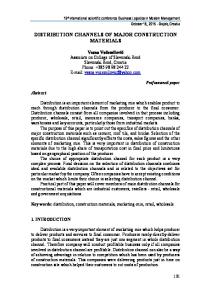
exit by a small producer from the traditional channel. Concretely, the small producer who becomes a large producer decreases its quantity distributed through the traditional channel, which allows producers who remain small to expand their quantities distributed through the s (w ) in (3) increases in M . Figure 1 shows a graphical example traditional channel; that is, qit r

of how the quantities change with an increase in M . [Figure 1 about here] l (w ) in (1) and q l (w ) in Proposition 1 When M is small such that wr ≥ w(N, M ), qir r r it l (w ) in (1) always (2) are independent of M . When M is large such that wr < w(N, M ), qir r l (w ) in (2) always increases with an increase in decreases with an increase in M , although qit r s (w ) in (3) always increases with an increase in M . M . qit r

The profits

First, when wr ≥ w(N, M ), the profit of each large producer, πil (wr ) in (6), is

constant because the producer does not supply through the traditional channel but supplies its product through external distribution channels as if it is a price taker whose selling price is wr . In contrast, the profit of each small producer, πis (wr ) in (7), monotonically increases with an increase in M because the exits by past small producers from the traditional channel increase the retail price of the traditional channel. From the upstream industry’s perspective, an increase in M monotonically increases the sum of the producers’ profits because an expansion of a small producer’s distribution channel simply works as a profit opportunity expansion within the industry. Second, when wr < w(N, M ), the profit of each large producer, πil (wr ) in (6), monotonically increases in M . This profit increase stems from an increase in the profit from the supply through the traditional channels from the mitigation of competition, which is related to the previous discussion on quantities. The profit of each small producer, πis (wr ) in (7), monotonically increases with an increase in M , which also comes from the mitigation of competition in the traditional channel. As in the case in which wr ≥ w(N, M ), an increase in M monotonically increases the sum of the producers’ profits. Note that the profit of each 13

small producer is higher than that of each large producer when the number of large producers is greater than a threshold value. This is because the inability of each small producer to supply its goods to external distribution channels functions as a commitment to a larger supply through the traditional channel, which induces large producers to produce less because of strategic substitutability and the convexity of production costs. Figures 2 and 3 summarize the change in profits. [Figures 2 and 3 about here] Proposition 2 When M is small such that wr ≥ w(N, M ), πil (wr ) in (6) is independent of M . When M is large such that wr < w(N, M ), πil (wr ) in (6) always increases with an increase in M . πis (wr ) in (7) always increases with an increase in M . The sum of the producers’ profits monotonically increases with an increase in M .

5

The main case (wr is endogenous)

Our main focus is to investigate how the number of large producers influences the equilibrium outcome through a change in wr . To do so, we investigate how an increase in M influences the endogenous values step by step: quantities, retail price, purchase price, profits, and total surplus.

The quantities

Except for a change in the purchase price, the basic properties of the main

case are shared with the benchmark case. As in the previous section, an increase in the number l (w ∗ ), except of large producers lowers the quantity supplied by each supplier to the retailer, qir r

˜b ≤ M ≤ M ˜ a . We, therefore, explain retailer pricing. An increase for the case in which M in M is a supply expansion of goods that allows the retailer to set a lower wr inducing each of the producers to produce less for the retailer. When M becomes larger than the threshold ˜ a , as in the previous section, each large producer supplies through both channels (see value M l (w ∗ ) in (13)). The quantity supplied by each small producer monotonically increases with qit r

an increase in M . Figure 4 shows a graphical example of how an increase in M influences the quantities. 14

[Figure 4 about here] l (w ∗ ) in (13) increases with an increase in M if M ≥ M ˜ a , otherwise, it is Proposition 3 qit r l (w ∗ ) in (12) decreases with an increase in M if M is on the range [0, M ˜ b ] or [M ˜ a , N ), zero. qir r s (w ∗ ) in (14) always increases with an increase otherwise, it increases with an increases in M . qit r

in M . Purchase price wr∗ and retail price p∗t

The purchase price wr∗ decreases with an increase

˜b ≤ M ≤ M ˜ a . Although the in the number of large producers, except for the case in which M quantity supplied by each large producer to the retailer decreases with an increase in M , the total quantity supplied increases, which allows the retailer to set a lower purchase price wr∗ . As in the previous section, a marginal increase in M functions as an exit (or a partial exit) by a small producer from the traditional channel, which enhances the profitability of the traditional channel. However, the continuous decrease in wr∗ through an increase in M diminishes the profitability increment from the traditional channel because the quantity reduction by large producers in the external channel allows the large producers to increase their quantities supplied through the traditional channel because of the production cost convexity. As a result, the marginal increment of the retail price in the traditional channel p∗t substantially decreases ˜ a . Figure 5 shows a graphical example of how an increase in M influences wr∗ when M ≥ M and p∗t .10 [Figure 5 about here] ˜ b ] or Proposition 4 wr∗ in (8) decreases with an increase in M if M is within the range [0, M ˜ a , N ), otherwise, it increases with an increase in M . p∗t in (15) always increases with an [M increase in M .

Profits and total surplus

˜ a , the profit of each large producer monotonically When M > M

decreases with an increase in M up to a threshold value of M and slightly increases with a 10 ˜ b, M ˜ a ], that is, those values are the same within the range In Figure 5, wr∗ and p∗t overlap on the range [M ˜ b, M ˜ a ] because each large producer just halts supply through the traditional channel. This implies that the [M ˜ b, M ˜ a ]. marginal revenues from the two channels are the same, that is, wr∗ = p∗t within the range [M

15

further increase in M . The former profit decrease stems from the substantial decrease in the purchase price wr , and the latter slight profit increase stems from an increase in the profit from the supply through the traditional channel, as in the previous section. Contrary to the change in each large producer’s profit, the profit of each small producer monotonically increases with an increase in M . This is correlated with an increase in the retail price of the traditional channel, as in the previous section. Additionally, the profit of each small producer is higher than that of each large producer when the number of large producers is greater than a threshold value. The reason is similar to that in the previous section. Moreover, the profit of a small producer decreases by expanding its distribution channel if M is large; that is, a small producer does not have an incentive to expand its distribution channel if there is a substantial number of existing large producers. When M is large, the beneficial commitment not to supply to the retailer is effective, and the profitability of the external channel is not great because the retailer sets a lower purchase price as M increases. We can show a sufficient condition that expanding a small producer’s distribution channel actually decreases the small producer’s profit. Distribution channel expansion by a small firm is detrimental to it if M ≥ N/3.11 Figure 6 shows a graphical example of how an increase in M influences πil (wr∗ ) and πis (wr∗ ). [Figure 6 about here] ˜ b] Proposition 5 πil (wr∗ ) in (10) decreases with an increase in M if M is within the range [0, M ˜ a , Mc ), otherwise, it increases with an increases in M , where or [M Mc ≡

(c + (1 + N )β)(2c + (1 + N )β)((2N − 1)c + (1 + N )β) . (3c + (1 + N )β)(2(1 + N )β 2 + (5 + 3N )cβ + 4c2 )

πis (wr∗ ) in (11) always increases with an increase in M . πis (wr∗ ) in (11) is larger than πil (wr∗ ) in (10) if M is larger than a threshold value. A small producer does not have an incentive to become a large producer if M ≥ N/3. 11

The profit deterioration occurs for more wide range of M . For instance, when α = 1, β = 1, N = 30, and c = 2, expanding the distribution channel is detrimental to a small producer if M ≥ 9, which is smaller than 30/3 = 10.

16

The sum of the producers’ profits can nonmonotonically change with an increase in M ˜ a , the partial because the purchase price wr∗ decreases with an increase in M . For M > M derivative of the sum with respect to M is given as ∂(M πil (wr∗ ) + (N − M )πis (wr∗ )) c(1 + N )α2 βE(c + (1 + N )β)2 = , ∂M D3 where D is defined in the previous section and E ≡ {c(c + (1 + N )β)((1 + N )2 β 2 + (2N 2 + 9N − 1)cβ + 2(3N − 1)c2 )} − {(1 + N )3 β 4 + (1 + N )(9 + 4N + 3N 2 )cβ 3 + (26 + 21N + 5N 2 + 2N 3 )c2 β 2 + 6(5 + N )c3 β − 4(N − 3)c4 }M . When M = N , the sign of the partial derivative is equivalent with that of −N (1 + N )3 β 3 − (1 + N )(−1 + 6N + N 2 + 2N 3 )cβ 2 − (1 + 11N + 2N 2 )c2 β + 2(−1 − 3N + 2N 2 )c3 , which is negative whenever c is not sufficiently large. That is, if the production function of each producer is not too convex, an increase in M can decrease the sum of the producers’ profits. Figures 7 and 8 show graphical examples of how an increase in M influences M πil (wr∗ ) + (N − M )πis (wr∗ ). Particularly, from Figure 8, we expect that, on a large parameter range of c, an increase in M will not enhance the total profit of the producers when large producers supply through the traditional channel as well as the external channel. The relation between the sum of the producers’ profits and M is quite different from that in the previous section. The relation in this section stems from the monotonic decrease in wr when M is large. The price decrease is applied to all the quantities supplied in the external channel, which substantially reduces the profits of large producers when M is large. This effect does not exist in the exogenous purchase price case (see the previous section). Note that, when M is small, the profit level in the main case is larger than that in the benchmark case in which wr is not large (see Figures 3 and 7). When M is positive and small, the total profit in the main case is larger than that in the benchmark case because the retailer sets a higher price when M is small. [Figures 7 and 8 about here] Proposition 6 The sum of the producers’ profits nonmonotonically changes with an increase in M when c is not sufficiently large. We discuss how the independence of the downstream markets influences the main results. 17

We could extend our demand system to the following: pi = α − βQi − γQj , (i, j = t, r, j ̸= i, and γ ∈ [0, 1)). This demand system nests our current demand system a special case (the case of γ = 0), although the analysis becomes substantially complicated. Under the extended demand system, distribution channel expansion directly reduces the market size in the traditional channel, which diminishes the quantities supplied by small producers. This implies that the importance of becoming a large producer intensifies as the substitutability of the two channels increases. We expect that the profit of each small producer is always smaller than that of each large producer if the substitutability of the two channels (γ) is high, in contrast with the result in the main model. We also expect that the nonmonotonicity of the total profits in the upstream would still hold because the purchase power of the retailer remains even under the extended demand system. The results in Sections 4 and 5 and the above brief discussion imply that we should seriously take into account the market structures when we consider distribution channel expansion in upstream industries. Finally, we briefly mention the total surplus property. Proposition 7 The total surplus, W ∗ , monotonically increases with an increase in M . Figure 9 shows a graphical example of how an increase in M influences W ∗ . [Figure 9 about here]

6

Conclusion

We consider a market with a vertical relation in which upstream producers produce their goods and then sell them through two distribution channels, a traditional channel and external retailers. We assume that some of the producers (small producers) are able to distribute their products only through the traditional channel, whereas the other producers (large producers) can distribute to both channels. We discuss the influence of the number of large producers on the equilibrium outcome. Given a fixed number of producers, we show several results: an increase in the number of large producers does not always improve the sum of producers’ profits when a for-profit 18

retailer, who can unilaterally set the purchasing terms, is the only external retailer; the profit of each large producer can be smaller than that of each small producer if there is a substantial number of large producers, and the profit of each producer increases with an increase in the number of large producers when the purchase price in the external channel does not change. These results imply that the effect of expanding distribution channels substantially depends on the market structure in the external channel. Agricultural cooperatives should consider their bargaining position when they sign agreements with nationwide retailers for cooperative distribution because the retailers tend to have strong bargaining power. The current model does not explicitly consider firm behavior in the traditional distribution channel in the sense that there is no active retailer in the traditional distribution channel. It would be reasonable to consider producers’ cooperatives (COOPs) in the traditional distribution channel as discussed in Fousekis (2015), who discuss mixed duopsony with a cooperative.12

7

Appendix

The appendix provides the proofs of the statements in the main text.

The proof of Remark 1

The difference is given by

˜a − M ˜b = M

2c2 (c + β)((N + 1)β + 2c) . β(3c + 2β)(2(1 + N )β 2 + (5 + 3N )cβ + 4c2 )

Differentiating it with respect to N , we have ˜a − M ˜ b) ∂(M 4c3 (c + β)2 =− < 0. ∂N (3c + 2β)(2(1 + N )β 2 + (5 + 3N )cβ + 4c2 )2 That is, the difference decreases in N . When N = 0, the difference is 2c2 (c + β)(2c + β) , β(3c + 2β)(2β 2 + 5cβ + 4c2 ) which is smaller than 1 if and only if 4β 4 + 16cβ 3 + 21c2 β 2 + 6c3 β − 4c4 > 0. Therefore, we have the statement in the remark. 12

As mentioned in Fousekis (2015, p.518-9), the extension is related to the discussion of mixed markets in which the objective functions differ among firms (e.g., a firm’s objective to maximize total surplus). For instance, in the context of the vertical relations as discussed in our paper, Matsumura and Matsushima (2012) and Chang and Ryu (2015) discuss mixed markets with vertical relations.

19

Proof of Proposition 1 to M , we have l (w ) ∂qir r ∂M

=

l (w ) ∂qit r ∂M

=

s (w ) ∂qit r ∂M

=

∂pt (wr ) ∂M

=

Differentiating the four values in (1), (2), (3), and (4), with respect

   − (c + β)((c + (N + 1)β)wr − cα) < 0 if wr < w(N, M ), β((M + 1)c + (N + 1)β)2   0 if wr ≥ w(N, M ),    (c + β)((c + (N + 1)β)wr − cα) > 0 if wr < w(N, M ), β((M + 1)c + (N + 1)β)2   0 if wr ≥ w(N, M ),  (c + (N + 1)β)wr − cα    ((M + 1)c + (N + 1)β)2 > 0 if wr < w(N, M ),  αβ   >0 if wr ≥ w(N, M ), (c + (N − M + 1)β)2  (c + β)((c + (N + 1)β)wr − cα)   > 0 if wr < w(N, M ),  ((M + 1)c + (N + 1)β)2  (c + β)αβ   >0 if wr ≥ w(N, M ). (c + (N − M + 1)β)2

Proof of Proposition 2

It is easy to find that πil (wr ) does not change with an increase in

M when wr ≥ w(N, M ). For M such that wr < w(N, M ), 2(c + β)((c + (N + 1)β)wr − cα)((c + β)α − (c + (N − M + 1)β)wr ) ∂πil (wr ) > 0. = β((M + 1)c + (N + 1)β)3 ∂M l (w ) and q l (w ) are positive when Note that, to check the sign, we use the condition that qir r r it

wr < w(N, M ). It is easy to find that πis (wr ) increases with an increase in M when wr ≥ w(N, M ). For M such that wr < w(N, M ), (α + M wr )(c + 2β)((c + (N + 1)β)wr − cα) ∂πis (wr ) > 0. = ((M + 1)c + (N + 1)β)3 ∂M l (w ) is positive when w < w(N, M ). Note that, to check the sign, we use the condition that qir r r

For M such that wr ≥ w(N, M ), the partial differential of (M πil (wr ) + (N − M )πis (wr )) with respect to M is given as ∂(M πil (wr ) + (N − M )πis (wr )) w2 α2 (c + 2β)((N − M − 1)β − c) = r + . ∂M 2c 2(c + (N − M + 1)β)3 We further differentiate it with respect to M , and we obtain α2 β(c + 2β)((N − M )β − 2(β + c)) . (c + (N − M + 1)β)4 20

(16)

Its sign is the same with that of the numerator which is monotonically decreasing in M . On the range of M such that wr ≥ w(N, M ), there are three possibilities on the sign of this numerator: (i) (+) for small M but (−) for large M ; (ii) (+) for all M ; (iii) (−) for all M . From the three possibilities, we find that the partial differential of (M πil (wr ) + (N − M )πis (wr )) is minimized at M = 0 or the highest value of M on the range of M such that wr ≥ w(N, M ), that is, M = ((β(N + 1) + c)wr + (β + c)α)/(βwr ). First, we check the sign of the partial differential in (16) when M = 0. The partial differential is minimized at the lowest value of wr in Assumption 1. When wr is the left-hand side of min in Assumption 1, the partial differential is α2 β(2N c2 + β(4N + 1)c + (N + 1)β 2 ) > 0. 2c(c + (N + 1)β)3 When wr is the right-hand side of min in Assumption 1, the partial differential is

8(c + (N +

α2 βF1 , + 1)c + N (N + 1)β)2

1)β)3 ((2N

where F1 ≡ 4(2N + 1)(5N 2 − 1)c3 + β(45N 4 + 92N 3 + 22N 2 − 12N − 3)c2 + (N + 1)(13N 4 + 48N 3 − 6N 2 − 8N + 1)β 2 c + 8(N − 1)N 2 (N + 1)2 β 3 (> 0). Second, we check the sign of the partial differential in (16) when M is the maximum value of wr ≥ w(N, M ), that is, M = ((β(N + 1) + c)wr + (β + c)α)/(βwr ). The partial differential is wr2 (β 2 α + 2c(α + wr )(c + 2β)) (> 0). 2cα(c + β)2 The partial differential of (M πil (wr ) + (N − M )πis (wr )) with respect to M is positive when wr ≥ w(N, M ). For M such that wr < w(N, M ), the partial differential of (M πil (wr ) + (N − M )πis (wr )) with respect to M is given as l (w )F ∂(M πil (wr ) + (N − M )πis (wr )) qir r 2 = , ∂M 2(c + β)((M + 1)c + (N + 1)β)2

where F2 ≡ {(2c + β)(c + (N + 1)β)2 wf − αc(2c2 + 5βc − (N − 3)β 2 )} + {(2c + 3β)αc2 − c(2c2 + 7βc + (N + 5)β 2 )wf }M . We now check whether F2 is positive when wr is on the range in Assumption 1. F2 is a linear function of M . We first check the sign of the constant term. Because this term is increasing in wf , this is minimized when wf is at the lowest value in 21

Assumption 1. Substituting the two possible lowest values in Assumption 1 into the constant term in F2 , we have (2c + β)(c + (N + 1)β)2 ·

(2(2N + 1)c + (N + 1)(3N + 1)β)αc 2(c + (N + 1)β)((2N + 1)c + N (N + 1)β) −αc(2c2 + 5βc − (N − 3)β 2 )

=

βαc{2(5N 2 − 1)c2 + (6N 3 + 15N 2 − 1)βc + (5N 3 + 3N 2 − N + 1)β 2 } (> 0), 2((2N + 1)c + N (N + 1)β) (c + β)α (2c + β)(c + (N + 1)β)2 · − αc(2c2 + 5βc − (N − 3)β 2 ) c + (N + 1)β

= βα{2N c2 + (4N + 1)βc + (N + 1)β 2 }(> 0). The constant term is always positive for any wr in Assumption 1. From this outcome and the linearity of F2 , if F2 is positive when M = N , then we can conclude that F2 is always positive. When M = N , F2 is F2 |M =N = α((N − 3)β + 2(N − 1)c)c − {2(N − 1)c2 + (N − 3)βc − (N + 1)2 β 2 }wf . This is a linear function of wf and the constant term is positive because N ≥ 3 by assumption. If this is positive when wf is at the lowest value and at the highest value, this linear function is positive for any wf in Assumption 1. Substituting the three values into wf in F2 |M =N , we have α((N − 3)β + 2(N − 1)c)c −{2(N − 1)c2 + (N − 3)βc − (N + 1)2 β 2 } · =

(2(2N + 1)c + (N + 1)(3N + 1)β)αc 2(c + (N + 1)β)((2N + 1)c + N (N + 1)β)

(N + 1)αβ(β + c)cF3 (> 0), 2(c + (N + 1)β)((2N + 1)c + N (N + 1)β) α((N − 3)β + 2(N − 1)c)c − {2(N − 1)c2 + (N − 3)βc − (N + 1)2 β 2 } ·

=

(c + β)α c + (N + 1)β

αβ(β + c){2N (N − 1)c2 + (2N 2 − N + 1)βc + (N + 1)2 β 2 } (> 0), c + (N + 1)β α((N − 3)β + 2(N − 1)c)c − {2(N − 1)c2 + (N − 3)βc − (N + 1)2 β 2 } · α

= (N + 1)2 αβ 2 (c + β)(> 0), where F3 ≡ {2(3N 2 − 2N − 1)c2 + (4N 3 + 7N 2 − 6N − 1)βc + (5N 3 + 3N 2 − N + 1)β 2 }(> 0). Therefore, F2 |M =N is positive, thus, F2 is positive. From the discussion, we can conclude that 22

the partial differential of (M πil (wr ) + (N − M )πis (wr )) with respect to M is positive under Assumption 1.

Proof of Proposition 3

l (w ∗ ) = 0 when M < M ˜ a . When M > M ˜ a, It is easy to find that qit r

l (w ∗ ) c(N + 1)α(c + β)(2c + (N + 1)β) ∂qit r = > 0. ∂M 2{(1 + N )M β 2 + ((1 + N ) + (2 + N )M )cβ + (1 + 2M )c2 }2 l (w ∗ )/∂M < 0 when M < M ˜ b and that ∂q l (wr∗ )/∂M > 0 when It is easy to find that ∂qir r ir

˜b ≤ M ≤ M ˜ a . When M > M ˜ a, M l (w ∗ ) ∂qir (N + 1)α(c + β)((1 + N )β 2 + (2 + N )cβ + 2c2 ) r =− < 0. ∂M 2{(1 + N )M β 2 + ((1 + N ) + (2 + N )M )cβ + (1 + 2M )c2 }2 s (w ∗ ). The first-order partial derivatives of We check how an increase in M influences qit r s (w ∗ ) with respect to M is given as qit r  (N + 1)αβc2  ˜a < M,  > 0 if M  s ∗ ∂qit (wr ) 2{(1 + N )M β 2 + ((1 + N ) + (2 + N )M )cβ + (1 + 2M )c2 }2 = αβ  ∂M  ˜ a.  >0 if M ≤ M (c + β + (N − M )β)2

Proof of Proposition 4

˜ b and that It is easy to find that ∂wr∗ /∂M < 0 when M < M

˜b ≤ M ≤ M ˜ a . When M ≥ M ˜ a, ∂wr∗ /∂M > 0 when M c(1 + N )αβ(c + β)(c + (1 + N )β) ∂wr∗ < 0. = − 2{(1 + N )M β 2 + ((1 + N ) + (2 + N )M )cβ + (1 + 2M )c2 }2 ∂M The partial derivative of p∗t with respect to M is given as  αβ(c + β)  ˜ a,  >0 if M < M  ∗ ∂pt (c + β + β(N − M ))2 =  c2 (N + 1)αβ(c + β) ∂M  ˜a ≤ M.  > 0 if M 2{(1 + N )M β 2 + ((1 + N ) + (2 + N )M )cβ + (1 + 2M )c2 }2 Proof of Proposition 5

˜ a, We check how an increase in M influences profits. For M > M

the partial derivative of πil (wr∗ ) with respect to M is given as ∂πil (wr∗ ) c(N + 1)α2 β(c + β)F4 = . ∂M 4(c + (1 + N )β){(1 + N )M β 2 + ((1 + N ) + (2 + N )M )cβ + (1 + 2M )c2 }3 where F4 ≡ (3c + (1 + N )β)(2(1 + N )β 2 + (5 + 3N )cβ + 4c2 )M − (c + (1 + N )β)(2c + (1 + ˜ a ) (F4 | N )β)((2N − 1)c + (1 + N )β). F4 is positive (negative) when M = N (M = M ˜a = M =M 23

−(N + 1)(c + β)(c + (N + 1)β)2 ). F4 = 0 when M=

(c + (1 + N )β)(2c + (1 + N )β)((2N − 1)c + (1 + N )β) = Mc . (3c + (1 + N )β)(2(1 + N )β 2 + (5 + 3N )cβ + 4c2 )

˜ b and that ∂π l (w∗ )/∂M > 0 when M ˜b ≤ M ≤ M ˜ a. Note that ∂πil (wr∗ )/∂M < 0 when M < M r i ˜ a , it is easy to find that ∂π s (w∗ )/∂M > 0. For M > M ˜ a, For M ≤ M r i ∂πis (wr∗ ) c2 (N + 1)α2 β(c + 2β)F5 > 0. = ∂M 4(c + (1 + N )β){(1 + N )M β 2 + ((1 + N ) + (2 + N )M )cβ + (1 + 2M )c2 }3 where F5 ≡ 2M (1 + N )β 2 + (2(1 + N ) + (5 + 3N )M )cβ + 2(1 + 2M )c2 > 0. ˜ a , the difference between the profits of small and large producers is given as For M > M πis (wr∗ ) − πil (wr∗ ) =

8(c + (1 + N )β){(1 +

c(N + 1)α2 βF6 , + ((1 + N ) + (2 + N )M )cβ + (1 + 2M )c2 }2

N )M β 2

where F6 ≡ (8c2 + 2(5 + 3N )cβ + 4(N + 1)β 2 )M − (2(N − 1)c2 + (2N 2 + N − 1)cβ + (N + 1)2 β 2 ). ˜ a (M = N ) (F6 | F6 is negative (positive) when M = M ˜ a = −(N + 1)β(c + (N + 1)β)). M =M Thus, there exists M such that F6 = 0. To prove the claim that a small producer does not have an incentive to expand its distribution channel if the number of large producers is large, we need to compare πis (wr∗ ) when M = k and πil (wr∗ ) when M = k + 1. If the former is larger than the latter, each small producer does not have an incentive to expand its distribution channel when M = k. The difference between the two values is given as πis (wr∗ )|M =k − πil (wr∗ )

M =k+1

=

c(N + 1)α2 βF8 , F7

where F7 ≡ 8(c + (1 + N )β){(1 + N )kβ 2 + ((1 + N ) + (2 + N )k)cβ + (1 + 2k)c2 }2 {(1 + N )(k +

24

1)β 2 + ((1 + N ) + (2 + N )(k + 1))cβ + (3 + 2k)c2 }2 and F8 ≡ a0 + a1 k + a2 k 2 + a3 k 3 , where a0 = −c2 {2(N + 1)c4 + 6(N 2 + 3)βc3 + 2(3N 3 − N 2 + 8N + 16)β 2 c2 +(2N 4 + N 3 + N 2 + 23N + 21)β 3 c + (N 4 + 2N 2 + 8N + 5)β 4 }, a1 = −2c{4(N − 2)c5 + 2(5N 2 − 10N − 4)βc4 +(8N 3 − 9N 2 − 34N + 5)β 2 c3 + (2N 4 + 5N 3 − 23N 2 − 19N + 11)β 3 c2 +(3N 4 − N 3 − 13N 2 − 3N + 6)β 4 c + (N 2 − 1)2 β 5 }, a2 = −{8(N − 7)c6 + 16(N 2 − 6N − 10)βc5 + 2(5N 3 − 20N 2 − 133N − 108)β 2 c4 +(2N 4 + 7N 3 − 129N 2 − 308N − 170)β 3 c3 +(5N 4 − 10N 3 − 121N 2 − 188N − 82)β 4 c2 +(N + 1)2 (4N 2 − 15N − 23)β 5 c + (N + 1)3 (N − 3)β 6 }, 2 a3 = 2{2c + (N + 2)βc + (N + 1)β 2 }2 {4c2 + (3N + 5)βc + 2(N + 1)β 2 }. The sign of the difference, πis (wr∗ )|M =k − πil (wr∗ ) M =k+1 , is the same with that of F8 . F8 is a continuous function of k, a0 < 0, and a3 > 0. We now prove that F8 > 0 when k ≥ N/3. To do it, we check the following: first, we show that F8 is convex in k on the range [N/3, N − 1]; second, we show that F8 is increasing in k on the range [N/3, N − 1]; finally, we show that F8 > 0 for k ∈ [N/3, N − 1]. First, we show the first matter. Because a3 > 0, it is sufficient to show that ∂ 2 F8 /∂k 2 is positive at k = N/3. Substituting k = N/3 into ∂ 2 F8 /∂k 2 , we obtain ∂ 2 F8 /∂k 2 |k=N/3 = 2{8(3N +7)c6 +40(N 2 +5N +4)βc5 +2(11N 3 +104N 2 +213N +108)β 2 c4 +(4N 4 +83N 3 +353N 2 + 452N +170)β 3 c3 +(11N 4 +110N 3 +285N 2 +268N +82)β 4 c2 +(N +1)2 (10N 2 +41N +23)β 5 c+ 3(N +1)4 β 6 }, which is positive. Second, we show the second matter. Because F8 is convex in k, it is sufficient to show that ∂F8 /∂k is positive at k = N/3. Substituting k = N/3 into ∂F8 /∂k, we obtain ∂F8 /∂k|k=N/3 = (2/3){4(2N 2 +11N +6)c6 +2(6N 3 +59N 2 +110N +12)βc5 +(6N 4 + 100N 3 +373N 2 +318N −15)β 2 c4 +(N 5 +32N 4 +226N 3 +449N 2 +227N −33)β 3 c3 +(3N 5 +51N 4 + 206N 3 + 267N 2 + 91N − 18)β 4 c2 + (N + 1)2 (3N 3 + 25N 2 + 29N − 3)β 5 c + N (N + 1)3 (N + 3)β 6 }, which is positive. Finally, we show the third matter. Because F8 is increasing in k, it is sufficient to show that F8 is positive at k = N/3. Substituting k = N/3 into F8 , we obtain F8 |k=N/3 = (1/27){(8N 3 + 96N 2 + 90N − 54)c6 + 2(4N 4 + 106N 3 + 339N 2 + 72N − 243)βc5 + 2(N 5 +72N 4 +479N 3 +657N 2 −261N −432)β 2 c4 +(33N 5 +467N 4 +1455N 3 +825N 2 −819N − 567)β 3 c3 + (N 6 + 76N 5 + 518N 4 + 878N 3 + 246N 2 − 324N − 135)β 4 c2 + N (N + 1)2 (2N 3 + 25

53N 2 + 105N − 18)β 5 c + N 2 (N + 1)3 (N + 9)β 6 }, which is positive. Therefore, F8 > 0 for k ∈ [N/3, N − 1]. Proof of Proposition 6

The discussion is presented in the main text.

Proof of Proposition 7

We check how an increase in M influences the total surplus. For

˜ a , the partial derivative of the total surplus with respect to M is given as M >M ) ( c(N + 1)α2 β(c + (N + 1)β)2 F9 ∗ ∂ M πil + (N − M )πis ∗ + πr∗ + CSt∗ + CSr∗ /∂M = , D3 where F9 ≡ 4(M (N − 1) + N )c4 + {3 + 15N + 8N 2 + 6M (−1 + 2N + N 2 )}βc3 + {6 + 20N + 18N 2 + 4N 3 + M (2 + 21N + 17N 2 + 2N 3 )}β 2 c2 + (1 + N ){3(1 + N )2 + M (7 + 16N + 5N 2 )}β 3 c + 3M (1 + N )3 β 4 . We easily find that the sign of the partial derivative is the same with that of ˜ a. F9 , which is plus. Therefore, the partial derivative is positive for any M > M ˜b ≤ M ≤ M ˜ a , the partial derivative of the total surplus with respect to M is given as For M

=

) ( 1 ∗ ∗ ∗ l∗ s∗ + π + CS + CS · ∂ M π + (N − M )π r t r /∂M i i α2 β c(2N c2 + β(2N 2 + 6N + 1)c + (2N 2 + 3N + 1)β 2 ) 2c2 (c + (N − M + 1)β)3 M (2c + β)(2c2 + β(2N + 5)c + 2(N + 1)β 2 ) − . 2c2 (c + (N − M + 1)β)3

˜ a , this is This is decreasing in M . When M = M ( ) ∗ ∂ M πil + (N − M )πis ∗ + πr∗ + CSt∗ + CSr∗ /∂M

˜a M =M

=

2c(N + 1)(c +

β)(2c3

8)c2

β 2 (N 2

+ β(3N + + + 7N + 7)c + (N 2 + 3N + 2)β 3 ) > 0. 4c2 + β(3N + 5)c + 2(N + 1)β 2

˜b ≤ M ≤ M ˜ a. Therefore, the partial derivative is positive for M ˜ b , the partial derivative of the total surplus with respect to M is given as For M < M

=

( ) 1 l∗ s∗ ∗ ∗ ∗ · ∂ M π + (N − M )π + π + CS + CS i i r t r /∂M α2 c(−c3 + β(5N − 3)c2 + β 2 (9N 2 + 18N + 1)c + 3β 3 (N + 1)3 ) 8(c + βM )2 (c + (N − M + 1)β)3 βc(13c2 + 2β(13N + 21)c + β 3 (9N 2 + 18N + 25)c)M − 8(c + βM )2 (c + (N − M + 1)β)3 (13β 2 c2 + β 3 (5N − 3)c − β 4 )M 2 + β 3 cM 3 . + 8(c + βM )2 (c + (N − M + 1)β)3 26

˜ b is not strictly positive if and only if c ≥ (N − 1)β. Thus, we do not need to Note that M ˜ b if c ≥ (N −1)β. From here on, we assume that c < (N −1)β. consider the case in which M < M To prove that the numerator is positive, we differentiate it with respect to M , and obtain −βc(13c2 +2β(13N +21)c+β 2 (9N 2 +18N +25))+(26β 2 c2 +2β 3 (5N −3)c−16β 4 )M +3β 3 cM 2 , which is convex in M and the first term is negative. Therefore, this is always negative if this ˜ b . Substituting M = M ˜ b into it, we obtain is negative at M = M −

4βc((N + 1)β + 2c)(24c3 + 4β(3N + 17)c2 + 2β 2 (11N + 30)c + β 3 (9N + 17)) (< 0). (3c + 2β)2

˜ b . If the numerator We find that the numerator is monotonically decreasing in M when M < M ˜ b , it is always positive for M < M ˜ b . When M = 0, the is positive at M = 0 and M = M numerator is c(−c3 + β(5N − 3)c2 + β 2 (9N 2 + 18N + 1)c + 3β 3 (N + 1)3 ), which is larger than c(−((N − 1)β)3 + β(5N − 3)(0)2 + β 2 (9N 2 + 18N + 1)(0) + 3β 3 (N + 1)3 )(> 0) because ˜ b , the numerator is 0 < c < (N − 1)β. When M = M 8c(β + c)((N + 1)β + 2c)2 (4c3 + β(2N + 11)c2 + 2β 2 (3N + 5)c + 3β 3 (N + 1)) (> 0). (3c + 2β)3 ˜ b . Therefore, the partial derivative is We find that the numerator is always positive for M < M ˜ b. positive for M < M

References [1] Agbo, M., D. Rousseli`ere, and J. Salani´e. 2015. “Agricultural Marketing Cooperatives with Direct Selling: A Cooperative-Non-Cooperative Game.” Journal of Economic Behavior & Organization 109(1): 56–71. [2] Ahn, J. and McQuoid, A.F. 2015. “Capacity Constrained Exporters: Identifying Increasing Marginal Cost.” mimeo, Department of Economics, Florida International University. [3] Albæk, S. and C. Schultz. 1998. “On the Relative Advantage of Cooperatives.” Economics Letters 59(3): 397–401. [4] Bulow, J.I., J.D. Geanakoplos, and P.D. Klemperer. 1985. “Multimarket Oligopoly: Strategic Substitutes and Complements.” Journal of Political Economy 93(3): 488–511. 27

[5] Chang, W.W. and H.E. Ryu. 2015. “Vertically Related Markets, Foreign Competition and Optimal Privatization Policy.” Review of International Economics 23(2): 303–319. [6] Chiang, W.K., D. Chhajed, and J.D. Hess. 2003. “Direct Marketing, Indirect Profits: A Strategic Analysis of Dual-Channel Supply-Chain Design.” Management Science 49(1): 1–20. [7] Coe, N.M. and M. Hess. 2005. “The Internationalization of Retailing: Implications for Supply Network Restructuring in East Asia and Eastern Europe.” Journal of Economic Geography 5(4): 449–473. [8] Fousekis, P. 2015. “Location Equilibria in a Mixed Duopsony with a Cooperative.” Australian Journal of Agricultural and Resource Economics 59(4): 518–532. [9] Fulton, M. and K. Giannakas. 2013. “The Future of Agricultural Cooperatives.” Annual Review of Resource Economics 5(1): 61–91. [10] Karantininis, K. and A. Zago. 2001. “Endogenous Membership in Mixed Duopsonies.” American Journal of Agricultural Economics 83(5): 1266–1272. [11] Kawamura, T., S. Kiyono, and S. Mitsuishi. 2011. “JA Hambai Jigyo Kaikaku: Case Year Book 2011.” (Japan Agricultural Cooperative Sales Operations Reforms: Case Year Book 2011 ), Zenkoku Nogyo Kyodo Kumiai Rengokai (JA Central Union of Agricultural Co-operatives): Tokyo (in Japanese). [12] Kawasaki, A., M.H. Lin, and N. Matsushima. 2014. “Multi-Market Competition, R&D, and Welfare in Oligopoly.” Southern Economic Journal 80(3): 803–815. [13] Matsumura, T. and N. Matsushima. 2012. “Airport Privatization and International Competition.” Japanese Economic Review 63(4): 431–450. [14] Matsushima, N. and R. Shinohara. 2014. “What Factors Determine the Number of Trading Partners?” Journal of Economic Behavior and Organization 106(1): 428–441.

28

[15] Matsushima, N. and L. Zhao. 2015. “Multimarket Linkages, Trade and the Productivity Puzzle.” Review of International Economics 23(1): 1–15. [16] Soderbery, A. 2014. “Market Size, Structure, and Access: Trade with Capacity Constraints.” European Economic Review 70(1): 276–298.

29

qlir Hwr L,qlit Hwr L,qsit Hwr L 0.05

qlir Hwr L

qsit Hwr L

0.04 0.03 0.02 qlit Hwr L

0.01 0

5

10

15

20

25

30

M

l (w ∗ ), q l (w ∗ ), q s (w ∗ ) qir r r r it it

Figure 1: Quantities (wr is exogenous) N = 30, α = 1, β = 1, c = 2

Πli Hwr L,Πsi Hwr L 0.0040 0.0035 Πsi Hwr L 0.0030 Πli Hwr L 0.0025 0.0020

0

5

10

15

20

25

30

M

πil (wr ), πis (wr ) Figure 2: The profits of large and small producers (wr is exogenous) N = 30, α = 1, β = 1, c = 2, wr = 1/10

30

MΠli Hwr L+HN-MLΠsi Hwr L 0.11 0.10 0.09 0.08 0.07 0.06 0

5

10

15

20

25

30

M

M πil (wr ) + (N − M )πis (wr ) Figure 3: The sum of the producers’ profits (wr is exogenous) N = 30, α = 1, β = 1, c = 2, wr = 1/10

quantity 0.07 qlir Hw*r L

0.06 0.05

qsit Hw*r L

0.04 0.03 0.02

qlit Hw*r L

0.01 5

10

15

20

25

l (w ∗ ), q l (w ∗ ), q s (w ∗ ) qir r r r it it

Figure 4: Quantities (wr is endogenous) N = 30, α = 1, β = 1, c = 2

31

30

M

p*t ,w*r 0.20 0.18 w*r

0.16 0.14

p*t

0.12 0.10 0.08 0.06 0

5

10

15

20

25

30

M

p∗t , wr∗ Figure 5: Retail price and purchase price (wr is endogenous) N = 30, α = 1, β = 1, c = 2

Πli Hw*r L,Πsi Hw*r L 0.0050 0.0045 Πli Hw*r L

0.0040 0.0035

Πsi Hw*r L

0.0030 0.0025 0.0020 0

5

10

15

20

25

30

M

πil (wr∗ ), πis (wr∗ ) Figure 6: The profits of large and small producers (wr is endogenous) N = 30, α = 1, β = 1, c = 2

32

MΠli Hw*r L+HN-MLΠsi Hw*r L 0.10 0.09 0.08 0.07 0.06 0

5

10

15

20

25

30

M

M πil (wr∗ ) + (N − M )πis (wr∗ ) Figure 7: The sum of the producers’ profits (wr is endogenous) N = 30, α = 1, β = 1, c=2 MΠli Hw*r L+HN-MLΠsi Hw*r L 0.18130

MΠli Hw*r L+HN-MLΠsi Hw*r L 0.18

0.18125

0.17

0.18120

0.16

0.18115 0.15 0.18110 0.14 0.18105 0.13 5

10

15

20

25

30

M

0

5

10

15

20

25

30

15

20

25

30

M

M πil (wr∗ ) + (N − M )πis (wr∗ ) (c = 20) MΠli Hw*r L+HN-MLΠsi Hw*r L 0.1778

MΠli Hw*r L+HN-MLΠsi Hw*r L

0.1777

0.17

0.1776 0.16 0.1775 0.15

0.1774

0.14

0.1773 5

10

15

20

25

30

M

0

5

10

M

M πil (wr∗ ) + (N − M )πis (wr∗ ) (c = 25) Figure 8: The sum of the producers’ profits (wr is endogenous) N = 30, α = 1, β = 1

33

W* 0.8

0.7

0.6

0.5

0

5

10

15

20

25

30

M

W∗ Figure 9: The total surplus (wr is endogenous) N = 30, α = 1, β = 1, c = 2

34