University of California, Berkeley Department of Economics
EC196: Topics in Economic Research Second Paper
What Determines Our Wage: The Econometric Analysis of Male-Female Wage Gap
Mentor: Shari J. Eli
EC196 Research Paper 2 Introduction The persistency of differentials by gender in the labor market is one of the key focus points of labor economics. Its importance in policy making is vast due to the necessity for mobility and heterogeneity of labor forces. It is important to know to which extent does gender play a role in determining wages, in order to target specific labor policies in the right direction. In addition, it is important to observe to which extent do other characteristics, such as race, nationality, religion or marital status, differently affect wages between men and women. As I demonstrate further in the paper, these differences indeed exist, and should be taken into consideration when forming future labor policies. The main purpose of this report is to examine the impact of gender and race in determining the hourly wage in UK. In an attempt to do so, I shall first analyze the literature on the topic, providing a short historical overview of the dynamics of the labor market discrimination. Afterwards, a quick analysis of the data is presented, outlining the main features and peculiarities of the dataset1. Furthermore, a model is estimated and its strengths and weaknesses are analyzed. Finally, I interpret and discuss the findings and potential policy implications that arise. Literature Analysis Economic discrimination in labor markets firstly needs to be defined. Modern economics literature conventionally defines it as the ‘presence of different pay for workers of the same ability’; or in other words, it is when equal productivity is not compensated by equal pay (Aigner and Cain, 1977: 175-77). Most popularly, a female/male wage gap is observed, although there are variations to this, particularly as a function of ethnicity. The black/white wage gap has been present ever since measurements on the topic have been conducted. The convergence of the black/white male wage gap during the 1960s and 1970s has been followed by a stagnation, which has continued now for almost 30 years (Altonji and Blank, 1999). Although I acknowledge that a number of other factors that can affect the amount a person is paid exist (such as previous unemployment, job characteristics, labor mobility, etc.), the focus of this paper will be
1
The data used is the UK Labour Force Survey, July – September, 2007 (LFS, 2007)
2
EC196 Research Paper 2 exclusively on the wage gap. Naturally, this might lead to a bias in the models presented; an issue I will also touch upon. One of the advantages of observing hourly wage in comparison to weekly or monthly wage is that it is more precise. Some surveys (for example, Drolet 2002 using Labour Force Survey 1997) show that men work more hours a week than females (43.1, in comparison to 39 for females), which leads to severe inaccuracies in estimated models of weekly wages. For this reason estimated regressions in the model I present take hourly wages as the dependent variable. Another interesting feature I shall explore is the effect of urban environment on wage gap. In particular, I shall observe whether there are differences between returns for men and women in urban settings (such as London and its outskirts), and the rest of the country. Phimister (2005) argues that the urban premium for women is larger than for men. Also, he concludes that married or cohabiting women have a substantially larger premium to those who are single. Such conclusion is consistent with the hypothesis that the market in urban areas, which is denser than that in rural, neutralizes the effects of lower spatial mobility (Phimister, 2005: 533). An important continuous variable in the model presented is years spent in education. In estimating the effect of an additional year spent in education, as well as differences between the returns for males and females, it would seem important to take into consideration the relatively recent expansion of higher education in UK. However, previous research shows that expansion has so far had no effect on the financial returns of education (Walker and Zhu, 2001: 145). Also, the same research shows that financial returns of education vary across subjects – those in Arts subjects tend to earn less than those in Economics, Management or Business related subjects. Regarding the male/female wage gap with respect to higher education, another interesting piece of research is that by Huang (1999). He argues that gender and education have a strong interactive influence on wages. All other things being equal, an additional year of education leads to higher wages for both men and women; however, above a certain level2, an additional
2
In his case, it is junior college – a non-bachelor secondary degree in the US. A UK equivalent would probably be a vocational degree.
3
EC196 Research Paper 2 year of education leads only to a larger increase in wage for females. As I shall argue later in the essay, this finding has important policy implications. Huang also mentions differences between countries. He notices that women3 in the UK earn 68 % as much as men; in France that figure is 79 %, whereas in Nordic countries it rises up to 89 %. My analysis will show whether there have been significant changes in the UK labor market since that period (mid-90s). Data Analysis: Figure 1: Overview of the Key Variables
Mean Median Maximum Minimum Std. Dev. Skewness Kurtosis Observations
Wage (£)
yredu
workex
12.751 10.430 512.67 0.020 10.577 17.721 719.76 7645
12.624 11.000 29.000 0.000 2.879 1.327 4.627 36716
9.534 6.083 68.00 0.083 9.658 1.458 4.918 28735
Table 1 shows an overview of the key continuous variables of the dataset. As only those who have finished their continuous education and are earning at the time of the survey are taken into consideration, the number of observations of wage is 7645. The average hourly pay is £12.75, with a standard deviation of 10.57. The median value is £10.43. Such a value, which is lower than the mean, suggests positive skewness. Such large positive skewness can probably be ascribed to a small number of individuals earning a lot more than the average.
3
Employment sector of his analysis is manufacturing, yet there should be no specific reason it could not be applied to the entire labour market.
4
EC196 Research Paper 2 Figure 2: Hourly Wage (adjusted for outliers)
Figure 3: Years spent in continuing education
As regards to education, the average person has spent 12 years in full time education, whereas the ‘middle person’ received the first 11 years of education (primary and secondary). An average individual has around nine and a half years of continuous work experience, ranging from a minimum of just a few months, to a maximum of almost 70 years. Figure 4: Key Variables by Sex/Race:
Sample Proportion (%) Average Years of Education Average Years of Work Experience Average Hourly Wage (£)
Female
Male
White
Other
40.10 12.54 7.91
59.90 12.67 10.37
92.85 12.47 9.79
7.15 14.24 6.49
10.84
13.97
12.85
11.43
Figure 4 shows that on average both females and males have been in continuous education for the same time; however, an average male has 3 years more work experience than an average female. He is also earning 22% more than she is. When observing differences across races, it can be seen that white individuals earn approximately 10 % more than those of other races (black, Chinese, Asian, etc.); despite the fact they have 1.5 years less education. Although this might seem unusual, we must take into consideration that Britain mostly issues work permits
5
EC196 Research Paper 2 for highly skilled workers, yet there remains a great deal of illegal, low skilled workers, who do not form part of the sample. Analysis of the estimated model: Equation (E1) in Figure 5 gives the results of the regression analysis of the wage determination. The dependent variable is natural logarithm of wages (a list of independent variables with explanations is provided in Appendix). The overall F-statistic is 286.23 (p < 0.001), which shows a significant relationship between the dependent and independent variables. Figure 5: Regression output for Equations E1 and E2 Dependent Variable: log(wage) Independent Variables c yredu 2
yredu workex 2 workex male white fulltime married london christian british financial male*yredu male*workex male*white male*fulltime male*married male*london male*christian male*british male*financial Adjusted R2 Number of Observations F-statistic
Equation E1 Equation E2 Coefficient Std.Error t-statistic Coefficient Std.Error t-statistic -0.500 0.127 -3.95*** -0.336 0.135 -2.48 0.241 0.017 13.49*** 0.240 0.018 13.16*** -0.005 0.024 -0.000 0.118
0.0006 0.002 0.000 0.013
-9.64*** 14,15*** -7.64*** 9.13***
-0.006 0.025 -0.0003 -0.107
0.0006 -8.88*** 0.002 13.99*** 0.000 -7.17*** 0.086 -1.25
0.233 0.223 0.079 0.271 0.019 0.079 0.136 -
0.023 0.016 0.011 0.020 0.013 0.020 0.018 -
10.03*** 13.69*** 6.71*** 13.56*** 1.44 3.84*** 7.57*** -
0.106 0.172 0.050 0.236 -0.002 0.053 0.125 -0.010 -0.001 0.192 0.134 0.044 0.049 0.029 0.032 0.024
0.033 0.017 0.017 0.028 0.020 0.031 0.022 0.004 0.001 0.046 0.039 0.023 0.039 0.026 0.041 0.033
0.298 7328 286.23
0.302 7328 173.76
Notes: *Statistically significant at p < 0.1; **statistically significant at p < 0.05; ***statistically significant at p < 0.01
6
3.16*** 9.81*** 2.87*** 8.52*** -0.09 1.67* 5.53*** -2.25** -0.96 4.18*** 3.42*** 1.88* 1.25 1.07 0.79 0.69
EC196 Research Paper 2 The model in E1 is tested for heteroskedasticity using the White heteroskedasticity test, and the results imply errors are robust (see section on Diagnostic Tests, p.10). This is in line with claims by Stock and Watson (2007: 165), who also conclude that regression errors in estimating log(wage) are robust. As it is obvious that men earn significantly more than women (11.8 % according to model in E1), I decided to test whether two separate regressions need to be done. In the case of homoskedastic errors, that can be done using a Chow test. However, in the case of heteroskedasticity, the following method is used - a new regression (E2) was formed, and the interactive dummy variables (between male and all other variables) were tested for joint significance. The Wald test is presented in Figure 8 (Diagnostic Tests, p.10). It shows that we reject the hypothesis that the joint significance of the interactive terms is 0. Thus there is a need for two separate regressions for males and females, in order to estimate a precise model. Figure 6: Regression output for Equations E3 and E4 Dependent Variable: log(wage) E3: MALE
E4: FEMALE
Independent Variables Coefficient Std.Error t-statistic Coefficient Std.Error t-statistic c yredu
-0.341 0.216
0.158 0.022
-2.17 9.72***
-0.603 0.277
0.215 0.030
-2.81 9.03***
-0.005 0.022
0.0007 0.002
-6.83*** -0.006 9.83*** 0.029
0.001 0.003
-6.42*** 9.80***
-0.0003
0.0006
-5.29*** -0.0005
0.0001
-5.10***
white fulltime
0.302 0.309
0.031 0.035
9.70*** 8.84***
0.107 0.171
0.033 0.017
3.17*** 9.74***
married london christian british financial
0.094 0.285 0.026 0.087 0.150
0.016 0.027 0.018 0.026 0.025
5.99*** 10.42*** 1.46* 3.34*** 5.90***
0.049 0.237 -0.002 0.049 0.124
0.017 0.027 0.020 0.031 0.022
2.81*** 8.59*** -0.14 1.56 5.46***
2
yredu workex workex
2
Adjusted R2 Number of Observations F-statistic
0.248 4463 143.67
0.323 2865 145.81
Notes: *Statistically significant at p < 0.1; **statistically significant at p < 0.05; ***statistically significant at p < 0.01
7
EC196 Research Paper 2 Regression E3 in Figure 6 shows the main wage determinants for males, whereas E4 outlines those applicable for females. As the variables yredu and workex have a non-linear effect on wages, I calculate the ‘optimum level’ of education. In other words, a level of education which maximizes earnings, can be determined by maximizing the partial differential as follows: For Male (E3):
For Female (E4):
! log(wage) = 0.216 + 2("0.005) yredu = 0 !yredu
! log(wage) = 0.277 + 2("0.006) yredu = 0 !yredu
yredu = 21.6
yredu = 23.1
This implies that earnings for males are maximized after 21.6 years of education, whereas for females they are maximized after 23.1 years, ceteris paribus. However, one must be careful and take these results with a degree of approximation, as they do not take other relevant variables that affect schooling into account (most importantly, the tuition fees). The interpretation of coefficients regarding education and work experience is as follows: For Male:
For Female:
! log(wage) = 0.216 + 2("0.005)10 = 0.116 !yredu
! log(wage) = 0.277 + 2("0.006)10 = 0.157 !yredu
! log(wage) = 0.216 + 2("0.005)20 = 0.016 !yredu
! log(wage) = 0.277 + 2("0.006)20 = 0.037 !yredu
A male with 10 years of education can expect a rise in his hourly wage of 11.6 % if he decides to take an extra year of education, whereas a female with the same level of education gets 15.7 % higher wage. After 20 years of education, a male earns 1.6 % more per hour for an additional year of education; whereas a female earns 3.7 % more. This confirms the research of Huang (1999), who concluded that females after a certain level of education earn more per each additional year of education than males.
8
EC196 Research Paper 2 With regard to work experience, the following analysis applies: For Male:
For Female:
! log(wage) = 0.022 + 2("0.0003)10 = 0.016 !workex ! log(wage) = 0.022 + 2("0.0003)20 = 0.01 !workex
! log(wage) = 0.029 + 2("0.0005)10 = 0.019 !workex ! log(wage) = 0.029 + 2("0.0005)20 = 0.009 !workex
After ten years of work experience, an average male’s salary will increase by 1.6 % after an additional year of work. For women, that number is higher – 1.9%. However, men’s returns on work experience diminish less over time. After twenty years of work experience, average male will get an increase of 1 % per additional year; whereas a woman gets only 0.9 %. Such analysis suggests that women have higher returns on work experience earlier in their careers. White men earn almost 30 % higher than men of other races. Amongst women, this gap is three times smaller. A white female earns 10.7 % more than a female individual, holding everything else constant. This suggests male/female gap is decreased amongst minorities, which is a very important fact. Regarding the nature of work, those male individuals working full-time have 30,9 % higher wages than those working part time; among women that gap is smaller. A woman working part time earns 17.1 % more than a woman in part-time employment. This study also shows that married men earn 9.4 % more than others (single, divorced, separated, widowed). Among women, that discrepancy is significantly lower – a married female earns only 4,9 % more than a non-cohabiting one. This is also noted by Korenman and Neumark (1990: 283-4), who argue that married man earn substantially more than those who are not married. Region of work is also an important element in wage determination. Working in London is significant for both males and females alike. An average male individual working in the London area (central, inner or outer) earns 28.5 % more than the ‘identical’ individual working
9
EC196 Research Paper 2 anywhere else in the country. A woman’s average hourly earning is 23.7 % higher in comparison to women of other regions, keeping other variables constant. This again shows that discrepancies among females are lower than among men. Interestingly, religion and nationality are statistically insignificant for women at 1%, 5% and 10% level. For males, religion is also insignificant, but nationality is not. A man of British nationality earns 8.7 % more than an individual of any other nationality, which is significant at 1% level. Finally, working in highly paid industries4, such as financial sector, yields 15 % higher wages for men, and 12.4 % higher wages for women, compared to those working in any other industry. Diagnostic tests and Potential Drawbacks of the Model: Figure 7: White Heteroskedasticity Test: Regression E1 (general): H0= homoskedasticity Chi2(80) 104.83
Probability
0.0328
Figure 8: Joint Significance Test Regression E2 (general with interaction terms) H 0 : !13 = !14 = !15 = !16 = !17 = !18 = !19 = ! 20 = ! 21 = 0 H1 : ! k " 0, k = 13,..., 21 Test Statistic F-statistic
Value 5.890120
df (9, 7278)
Probability 0.0000
Figure 9: Ramsey (I) Reset Test Regression E3 (Males): H0= model has no omitted variables F-statistic (3,4448) 1.05 Probability
0.3711
Do not reject H0. Regression E4 (Females): H0= model has no omitted variables F-statistic (3,2850) 3.31 Probability
0.00192
Reject H0.
4
Industries used in this analysis: Financial Services, Business, Computer Science, Research and Development
10
EC196 Research Paper 2 A number of diagnostic tests were conducted to test the validity of this model. As mentioned previously, the initial model (E1) was tested by White test to prove the existence of heteroskedasticity robust standard errors. All of the regressions conducted are therefore adjusted for robust errors. Ramsey (I) Reset test was conducted to test for misspecification or omitted variable bias in Equations E3 and E4 (i.e. regressions on males and females respectively). The model for males ‘passes’ the test, and we reject the hypothesis that the model suffers from misspecification. On the other hand, the model for females, according to the test, suffers from misspecification. However, two facts must be taken into consideration. Firstly, that there are omitted variables in this model, such as those which are hard or impossible to measure (i.e. ability, previous family history, etc.). Secondly, Ramsey Reset Test is a low power test, therefore it need not necessarily hold true. I would argue that the main flaw of the models I presented is omitted variable bias. In particular, the lack of more precise data on family background and ability cause the estimates on other variables to be biased. In further research, it would be interesting to see how these variables affect wages across different subsamples (i.e. male/female, white/other, British/non-British). It could be useful to try to instrument for these variables, yet the particular dataset I was using seemed to lack any good instruments. For family background, potential instrument could be parent’s earnings or level of education, while ability would be very hard to instrument for in such a large sample. Another setback of my model is that it fails to explain the rationale behind the wage gap. Although I can speculate on reasoning behind the wage gaps, my particular models can not give a definitive answer. Although there is a certain range of literature that attempts to cover this field, I believe there is still lot of unknowns in this research area, and we can expect more discoveries in the future.. For instance, and interesting forthcoming paper by Ichino and Moretti (2008) attempts to look at female absenteeism caused by menstrual cycle as one of the causes of the wage gap. An interesting conclusion they make is that if women did not suffer menstrual symptoms, the wage gap would be 14.1% lower.
11
EC196 Research Paper 2 Policy implications: Despite the fact that both of the models do not have a very high Adjusted R2, there are still some implications and conclusions that can be drawn. The most important fact that can be seen across all the variables is that the females’ salary tends to be less affected by different influences. That is something government should take into account when drawing up policies. For example, the fact that nationality and religious affiliation have no statistical significance among women is a noteworthy fact. It means that when government is fighting discrimination on the basis of nationality or religion in the labor market, it needs to focus to men. However, overall, women are still highly discriminated at the labor market. They still earn substantially less than men (10-12 %), as the output from E1 and E2 shows. But they also benefit more from education. Therefore government’s educational policies should be more proactive towards woman, as that has the ability to contribute towards narrowing the male/female wage gap (see, for example, Huang, 1999). As part time workers earn considerably less than full time workers, government should try to increase the number of full time employment opportunities, relative to part time. Not only can policies be directed towards the labor force, but also towards companies that can be encouraged to employ workers full time, rather than part time. In the mean time, the profile of the part-time workers needs to be established, as it is highly likely that a large part of that population might be parents, or young parents, who can not afford to work while raising children. In such cases, government should intervene as well. Due to the fact that married men (and to a lesser extent women) tend to earn significantly more than those who are not married, government should be prepared for changes in the demographical and social structure. Marriage boosts productivity (Korenman and Neumark, 1990); however, due to the urban lifestyle, less people are getting married. Thus present and future governments need to adapt to the changing social structure, particularly regarding the social status.
12
EC196 Research Paper 2 Finally, governments should have more specific rules regarding the labor force working in London, as their salaries differ largely than those of other parts of the country. Firstly, some national policies (such as the minimum wage policy) need to be adapted to the more expensive lifestyle in London (or the cheaper one in rural areas). Secondly, as the area around London is vastly overcrowded, due to the migration of a population wanting higher salaries, the government needs to enhance policies that would encourage people to remain in the rural areas, or smaller towns. Conclusion: In summary, this paper analyzed the main determinants of wage. The main emphasis was on the male/female gap, and its implications on a number of different variables. The findings show that there is still a significant wage gap between men and women. What is also important is that male wages tend to be affected more by different variables (such as religion or nationality). Although both men and women tend on average to have the same level of education, women tend to earn more for each additional year of education they take. However, this is only true in the early parts of their careers. Men tend to be more affected by their marital status – being single diminishes their productivity and wage level. Women are, on the other hand not affected by their marital status. Such conclusions mean that there is not only a wage gap between men and women, but also a considerable difference between different aspects affecting their wages. For such reasons, as well as for large discrepancies in different areas of the country, the government should have very specific and targeted labor policies, as otherwise, it will not accommodate to such divergence.
13
EC196 Research Paper 2
Appendix: Variable Names and Explanations: yredu – number of years spent in education5 workex – number of years of work experience6 male. where 1 if male 0 otherwise
white, where 1 if white by ethnicity 0 otherwise (mixed, Asian, black, Chinese or other
fulltime, where 1 if employed fulltime 0 otherwise
married, where 1 if married 0 otherwise (single, separated, divorced, widowed, etc.)
london, where 1 if region of work is London (central, inner or outer) 0 otherwise
christian, where 1 if religious denomination is Christian 0 otherwise (Buddhist, Hindu, Jewish, Muslim, Sikh, any other religion, no religion at all)
british, where 1 if British by nationality 0 otherwise
financial, where 1 if employed in business & finance sector, computer science or R&D 0 otherwise
5
yredu = (age when leaving education – 5) workex = variable obtained using variable from the Labour Force Survey empmon (length of time in continuing employment in months), and dividing it by 12 6
14
EC196 Research Paper 2 Bibliography: Aigner, Dennis J. and Glenn G. Cain (1977), ‘Statistical theories of discrimination in labor markets’, Industrial and Labor Relations Review, 30: 175-187 Atlonji, Joseph G., and Rebecca Blank (1999), 'Race and Gender in the Labour Market' in Handbook of Labor Economics Volume 3C, Amsterdam: Elsevier Science B.V, pp. 3143-3259 Drolet, Marie (2001), ‘The Male-Female Wage Gap’, Perspectives on Labour and Income, Vol.2, No.12, pp. 5-13 Huang, Tung-Chun (1999), ‘The impact of education and seniority on the male-female wage gap: is more education the answer?’, International Journal of Manpower, Vol.20, No. 6, pp. 361-374 Ichino, Andrea and Enrico Moretti (2009), ‘Biological Gender Differences, Absenteeism and the Earnings Gap’, American Economic Journal: Applied Economics, Vol.1, Issue 1, January 2009 Korenman, Sanders and David Neumark (1990), ‘Does Marriage Really Make Men More Productive?’, The Journal of Human Resources, Vol.26, No.2, pp. 282-307 LFS (2007), Labour Force Survey, July-September 2007 Phimister, Euan (2005), ‘Urban effects on participation and wages: Are there gender differences?’, Journal of Urban Economics, No. 58, pp.513-536 Stock, James H. and Mark W. Watson (2007), Introduction to Econometrics, 2nd Edition, London: Pearson Education Walker, Ian and Zhu, Yu (2003), ‘Education, earnings and productivity: recent UK evidence’, Labour Market Trends, Vol.111, Issue 3, p.145
15