What Can We Learn about Neighborhood Effects from the Moving to Opportunity Experiment?1 Jens Ludwig University of Chicago

Jeffrey B. Liebman Harvard University

Jeffrey R. Kling Brookings Institution

Greg J. Duncan University of California, Irvine

Lawrence F. Katz Harvard University

Ronald C. Kessler Harvard Medical School

Lisa Sanbonmatsu National Bureau of Economic Research

Experimental estimates from Moving to Opportunity (MTO) show no significant impacts of moves to lower-poverty neighborhoods on adult economic self-sufficiency four to seven years after random assignment. The authors disagree with Clampet-Lundquist and Massey’s claim that MTO was a weak intervention and therefore uninformative about neighborhood effects. MTO produced large changes in neighborhood environments that improved adult mental health and many outcomes for young females. Clampet-Lundquist and Massey’s claim that MTO experimental estimates are plagued by selection bias is erroneous. Their new nonexperimental estimates are uninformative because they add back the selection problems that MTO’s experimental design was intended to overcome. INTRODUCTION

Experimental analyses of the data from the “interim evaluation” of the Department of Housing and Urban Development’s Moving to Oppor1

Support for this research was provided by grants from the National Science Foundation to the National Bureau of Economic Research (9876337 and 0091854) and the National Consortium on Violence Research (9513040), as well as by the U.S. Department of Housing and Urban Development (HUD), the National Institute of Child 䉷 2008 by The University of Chicago. All rights reserved. 0002-9602/2008/11401-0005$10.00

144

AJS Volume 114 Number 1 (July 2008): 144–88

MTO Symposium: What Can We Learn from MTO? tunity (MTO) housing mobility experiment, which measured outcomes for participating adults and children four to seven years after random assignment, find no significant impacts on adult economic outcomes from the opportunity to move to lower-poverty neighborhoods (Orr et al. 2003; Kling, Liebman, and Katz 2007). In an article in this issue, Susan ClampetLundquist and Douglas Massey (hereafter “CM”) reassess the MTO experimental estimates and present new nonexperimental estimates of neighborhood impacts on economic self-sufficiency. We are delighted that CM have undertaken a reanalysis of data from the MTO interim evaluation. One of our teams’ key goals in partnering with HUD and Abt Associates to fund, design, and implement the interim MTO study was to contribute to the research infrastructure available for studying neighborhood effects. A discussion about what the MTO data imply about neighborhood effects is exactly the type of exchange we hoped reanalysis of the MTO data would engender. We are particularly pleased that this reanalysis has been carried out by CM, since Clampet-Lundquist has previously collaborated with two members of our team (Duncan and Kling) on qualitative studies of MTO adult employment and the behavior of young people, and we hold Massey in the highest esteem for his many distinguished scholarly contributions. The basic arguments developed by CM are as follows: MTO was a weak intervention for studying neighborhood effects because the experiment was focused on generating residential integration by social class rather than by both class and race. The low-poverty but predominantly minority neighborhoods into which most MTO movers relocated are not capable of producing substantial improvements in the economic outcomes of MTO families. Moreover, the fact that many families who were offered the chance to relocate through the MTO program did not do so, and that some MTO movers subsequently moved to higher-poverty areas on their Health and Development and the National Institute of Mental Health (R01-HD40404 and R01-HD40444), the Robert Wood Johnson Foundation, the Russell Sage Foundation, the Smith Richardson Foundation, the MacArthur Foundation, the W. T. Grant Foundation and the Spencer Foundation. Additional support was provided by grants to Princeton University from the Robert Wood Johnson Foundation and from NICHD (5P30-HD32030 for the Office of Population Research), by the Princeton Industrial Relations Section, the Bendheim-Thomas Center for Research on Child Wellbeing, the Princeton Center for Health and Wellbeing, the National Bureau of Economic Research, and a Brookings Institution fellowship supported by the Andrew W. Mellon foundation. Thanks to Susan Clampet-Lundquist, David Deming, Lisa Gennetian, Harold Pollack, and seminar participants at the University of Chicago, Harvard, and the Population Association of America meetings for helpful comments and assistance. The MTO data used in this article are from HUD. The contents of this comment are the views of the authors and do not necessarily reflect the views or policies of HUD or the U.S. government. Direct correspondence to Jens Ludwig, University of Chicago, 969 East 60th Street, Chicago, Illinois 60637. E-mail: [email protected]

145

American Journal of Sociology own, compromises the demonstration’s experimental design by imparting selection bias to estimates of the MTO intervention’s effects. CM’s new nonexperimental analysis of the MTO data suggests a substantial positive “association” between time spent in low-poverty neighborhoods and adult economic outcomes which, combined with evidence from other research, makes it likely that neighborhoods do have important impacts on these outcomes. We respectfully disagree with each of the main methodological and substantive points developed by CM. To date, most of our team’s writings on MTO have focused on presenting and interpreting the main experimental impacts of the demonstration.2 We have not discussed in print any of the broader questions raised by CM’s article about alternative research methodologies or more fundamental implications of the MTO evaluation for theories of neighborhood effects. So we are grateful to the editor of AJS for giving us the opportunity to discuss these issues. In what follows, we address three main points. First, we clarify what can and cannot be learned from a randomized policy experiment with partial compliance. We show that features of MTO that lead to what CM describe as “selection bias” do not bias estimates from a properly executed experimental analysis of the MTO data. Their claim seems to reflect some misunderstanding about the calculation of experimental estimates or what is conventionally meant by selection bias. We focus on two types of estimates that follow from MTO’s experimental design—termed “intent to treat” and “treatment on the treated” in the experimental literature. Roughly speaking, the MTO intent-to-treat (ITT) effect on a given outcome is the simple difference between the outcome for all individuals assigned at random to MTO’s experimental condition, regardless of whether they “complied” by actually moving through MTO to a lowpoverty neighborhood, and the outcome for all individuals assigned to the control group. In contrast, the treatment-on-the-treated (TOT) estimates are of outcome differences for families actually moving in conjunction with the program. We show that neither ITT nor TOT estimates are biased by the fact that only some families moved through MTO or by the fact that not all movers stayed in low-poverty areas. Both estimators are informative about the existence of neighborhood effects on behavior, contrary to the distinction CM make between estimating “policy treatment effects” and “neighborhood effects.” 2 For results derived from the interim MTO evaluation, see Orr et al. (2003), Kling, Ludwig and Katz (2005), Sanbonmatsu et al. (2006), Kling et al. (2007), and Ludwig and Kling (2007). Various members of our team were also involved in studying MTO participants from individual demonstration sites over the short term (see Katz, Kling, and Liebman 2001; Ludwig, Duncan, and Hirschfield 2001; Ludwig, Ladd, and Duncan 2001; and Ludwig, Duncan, and Pinkston 2005).

146

MTO Symposium: What Can We Learn from MTO? Second, we discuss whether the neighborhood differences generated by MTO are large enough to tell us anything useful about neighborhood effects. We show that CM’s classification of neighborhoods into “low” and “high” poverty groups on the basis of a single 20% poverty rate threshold overstates the degree to which subsequent mobility by families moving through the MTO program waters down the MTO “treatment dose.” Despite subsequent mobility, the average neighborhood environments of families moving through the program differed greatly from the neighborhoods of their control-group counterparts in terms of neighborhood socioeconomic status (SES), crime, and collective efficacy, but not in terms of race. What to make of the limited MTO impacts on neighborhood racial integration? CM argue that because these new communities are lower poverty but still overwhelmingly minority, they should not be expected to change the behavioral outcomes of MTO families. This claim seems inconsistent with the original theories of neighborhood effects that motivated the MTO experiment, such as that of Wilson (1987), and also with evidence of sizable MTO impacts on other important outcomes, including mental health, some indicators of physical health, and violent behavior among adolescents (Kling et al. 2005; Kling et al. 2007). Perhaps one might argue that moving to a neighborhood that is both low poverty and majority white non-Hispanic is particularly important for improving economic outcomes. But that argument is inconsistent with CM’s new nonexperimental estimates, which, if taken at face value, suggest that the effects on economic outcomes of living in segregated versus integrated low-poverty tracts are indistinguishable. The third point of our article is to consider whether anything useful can be learned about neighborhood effects from the new nonexperimental estimates presented by CM. The answer, in our judgment, is no. We are sympathetic to CM’s goal of understanding how the effects of MTO vary by time spent in low-poverty neighborhoods. In any experiment, some subjects will benefit more than others. Understanding how and why benefits vary across program participants can help inform policy design. But CM’s approach reintroduces all of the selection problems that MTO’s randomization was designed to overcome. Even taken at face value, the associations CM document are overstated, because their analysis confounds cohort and time effects with neighborhood effects, and they perform the wrong hypothesis test for determining whether extra time spent in a low- rather than high-poverty area improves adult economic outcomes. CM measure economic outcomes at a single point in time using data from the interim MTO survey. Random assignment occurred over the four-year period between 1994 and 1998. Our previous work suggests that earlier cohorts of movers may have benefited 147

American Journal of Sociology more than later cohorts with respect to some outcomes, even when time since random assignment is held constant. Because CM’s key explanatory variable is the number of months spent in a low-poverty census tract, their analysis confounds differences in neighborhood effects by randomization cohort with changes in impacts by time spent in low-poverty areas. We show that when we replicate their analysis but control for total number of months between random assignment and the time of the interim survey, there is no evidence that extra time spent in low-poverty integrated neighborhoods improves economic outcomes, while the estimated effects of time in low-poverty segregated neighborhoods are quite small. We also find no evidence that living in low-poverty neighborhoods in general (pooling segregated and integrated areas together) improves economic outcomes. We do not mean to imply that we oppose any attempt to go beyond a pure experimental ITT or TOT estimate of MTO’s impact. On the contrary, we believe there can be great value in such analyses, but only as long as they are carried out in a way that still capitalizes to the greatest extent possible on the strengths of MTO’s experimental design. We provide an example of an instrumental variables (IV) analysis of the effect of neighborhood poverty on employment that takes advantage of MTO random assignment. More definitive evidence on the connection between time spent in lowpoverty neighborhoods and economic outcomes will require longer-term follow-up data on MTO participants as well as analyses that exploit the random assignment design of the MTO experiment. That is the plan for the long-term evaluation of MTO that is currently under way. We look forward to sharing these data and results in the future with members of the research and policy communities interested in neighborhood effects.

AVOIDING SELECTION BIAS USING RANDOMIZED EXPERIMENTS

In this section, we review the main challenges associated with identifying causal neighborhood effects on behavior and then discuss what randomized mobility experiments can—and cannot—accomplish. CM’s article introduces some confusion about the proper interpretation of published MTO estimates because it repeatedly refers to “sources of selection bias” in the experiment, caused by the failure of some families to move through the MTO program or to stay in low-poverty areas. We now discuss why a properly conducted experimental analysis of neighborhood effects using MTO data does not suffer from selection bias.

148

MTO Symposium: What Can We Learn from MTO? Challenges to Nonexperimental Estimation Nonexperimental analyses of neighborhood effects using data on individuals typically proceed by regressing an outcome of interest on measures of a given person’s neighborhood and individual characteristics.3 Outcomes that have been studied in this way range from earnings to teen childbearing and frequency of asthma attacks (see, e.g., Jencks and Mayer 1990; Aber, Brooks-Gunn, and Duncan 1997; Leventhal and Brooks-Gunn 2000; Sampson, Morenoff, and Gannon-Rowley 2002; Ellen and Turner 2003). The neighborhood variables tend to be those easily measured from the decennial census, such as census tract–level poverty rates or %minority, although in some cases extraordinary data collection efforts provide additional measures of such key constructs as neighborhood collective efficacy (Sampson, Raudenbush, and Earls 1997). Individual-level control variables include standard demographic characteristics such as age, education, and race, but may also include more detailed measures of family functioning. The key problem plaguing nonexperimental approaches is classic omitted-variable bias: people choose or in other ways end up in neighborhoods for reasons that are difficult to measure and that may also correlate with their outcomes. Neighborhood selection bias is difficult to avoid with nonexperimental analysis, because there will inevitably be individual characteristics left out of the regression that affect the outcome variable and that may also be related to neighborhood sorting. For example, a person’s level of competence or initiative may affect labor-market outcomes. If these factors also help determine where a person lives but are omitted, then the estimated coefficient on the neighborhood variable will reflect not only the impact of the neighborhood on the outcome but also the impact of the omitted variables that are correlated with both the neighborhood variable and the outcome. If unmeasured initiative both causes a person to find an apartment in a better neighborhood and boosts earnings, then the estimated impact of neighborhood conditions on earnings will be overstated. But downward bias is possible as well. For example, if parents of a child with learning disabilities move to a higher-income neighborhood in the hope of receiving better special-needs services but the researcher fails

3 Alternative approaches include attempts to estimate the scope of neighborhood effects using, e.g., correlations in outcomes among children or adults growing up or living in the same neighborhood (Solon, Page, and Duncan 2000), excess variation across areas in outcomes beyond what can be explained by variation in observable individual background characteristics (Glaeser, Sacerdote, and Scheinkman 1996), or differences in the size of the individual- vs. aggregate-data elasticity of some behavior to some measure of incentives or information (Glaeser, Sacerdote, and Scheinkman 2003).

149

American Journal of Sociology to measure the child’s history of learning disabilities, then the child’s attainment may in fact be boosted by the move but still be lower than observationally similar children whose families did not move to better neighborhoods. In this case, the estimated impact of neighborhood conditions on educational outcomes would be understated. Thus the curse of omitted-variable bias owing to neighborhood selection: neither the magnitude nor even the direction of selection bias is certain. So we cannot even bound the true neighborhood effect from nonexperimental estimates that are susceptible to selection bias. The use of longitudinal data to control for unobserved individual- or family-level time-invariant factors, through either standard panel-data fixed-effects models or their close cousins in the hierarchical linear model (HLM) realm, does not solve these problems. Fixed-effects or trajectory models identify neighborhood effects for subjects who change neighborhood residence over time. But if, say, families move from high- to lowpoverty areas in response to changes in hard-to-measure family circumstances related to initiative, children’s learning needs, or other factors, then selection biases persist. Although these selection concerns are well known, the standard nonexperimental approach remains the workhorse research design in the field. The obvious reasons are the ready availability of nonexperimental national surveys and the dearth of public-use data from randomized experiments. A growing number of social science studies rely on identifying “natural experiments” that generate plausibly exogenous variation in independent variables of interest, but this approach has proved challenging in the case of neighborhood environments. A second problem that plagues the nonexperimental literature is our lack of knowledge of which neighborhood characteristics matter for a particular outcome, in addition to our inability in most data sets to capture anything other than the coarsest measures of neighborhood environments. Suppose it is the poverty rate in a person’s apartment building, and not in the rest of the census tract, that determines outcomes. Or suppose the job network to which a person is exposed is a function of the number of different employers employing not only people in that person’s census tract but also people at that person’s church. If we put the wrong neighborhood characteristic on the right-hand side of the regression, we could erroneously conclude that neighborhood effects do not matter. This is a particularly difficult challenge in nonexperimental research, because the specific neighborhood variables that will be most important, and even the relevant geographic or social definition of “neighborhood,” may depend on the specific outcome that is being studied. 150

MTO Symposium: What Can We Learn from MTO? What a Randomized Intervention Can Achieve A randomized mobility intervention that induces otherwise identical groups of people to live, on average, in different types of neighborhoods solves both problems with respect to detecting the existence of neighborhood effects on the outcomes of interest. Randomization eliminates the need to correctly specify which neighborhood characteristic matters for each outcome to learn about whether neighborhoods matter. A mobility intervention changes an entire bundle of neighborhood characteristics, and the total impact of changing this entire bundle on any outcome can be estimated even if the researcher does not know which neighborhood variables matter. Randomization also solves the selection problem, by causing the variation in neighborhood of residence to occur for reasons that are uncorrelated with individual characteristics, whether or not those characteristics are measurable. In the following discussion, we emphasize intuition over precision. But since part of our disagreement with CM stems from differences in what we mean by the term “selection bias,” we include a more formal development of these issues in the appendix. Our main experimental results come from comparing the outcomes of all of the families randomized into the treatment group with those of all of the families randomized into the control group (i.e., ITT analysis).4 Because randomization ensures that the families in the two groups would have had, on average, identical outcomes in the absence of the experimental intervention, any differences that occur between the two groups can be attributed to the experimental intervention, which in this case was the offer of a geographically restricted housing voucher and housing mobility counseling. CM wonder how these ITT analyses can be informative about the existence of neighborhood effects, given the range of neighborhood environments experienced by families within the MTO experimental group (p. 128). The key to our experimental evaluations of MTO is that random assignment to the experimental group generates large differences in average neighborhood attributes with the control group, as we document below. If neighborhoods matter, these large differences in average neighborhood attributes should lead to differences in average economic or other outcomes. So while CM make a distinction between understanding the

4 We refer to the former as, interchangeably, “experimental-group” or “treatment-group” families. In the MTO experiment there were actually two experimental groups—one required to move to low-poverty neighborhoods and the other offered Section 8 (housing choice) vouchers. While we initially follow CM in focusing only on the experimental and control groups, having data on the Section 8 group is of great value, particularly for efforts to sort out the mechanisms through which MTO influences economic or other outcomes, as we discuss further below.

151

American Journal of Sociology effects of the MTO “policy treatment” and understanding “neighborhood effects,” experimental estimates of MTO treatment effects are informative about the existence of neighborhood effects even when there is variation in neighborhood environments within the experimental and control groups. It is true that the differences in average neighborhood characteristics between the experimental and control groups are generated by very heterogeneous processes. Some experimental-group families used the vouchers they were offered and some did not. Adopting the language of medical trials, in which people are randomly assigned to take medicines but some do not obey the doctors’ instructions, social scientists studying randomized experiments call people who take the offered service “compliers” and those who do not take advantage of the service “noncompliers.” CM correctly note that compliance was “highly selective” (p. 138) in the sense that the compliers and noncompliers are quite different from one another, as we (Kling et al. 2007) and others (Shroder 2002) have documented in previous work. However, CM are mistaken when they claim that partial compliance in MTO introduces “another potential source of selection bias into the experiment” (p. 121). Their claim seems to reflect some confusion either about the mechanics of how an ITT estimate is calculated or else about the meaning of selection bias as conventionally used in social science. Given this confusion, it might be useful to consider the logic of ITT estimates more closely. The fact that only some MTO families assigned to the experimental group comply with their treatment assignment and relocate through the program does not introduce any selection bias to an estimate of the effects of being offered MTO vouchers, because the control group is comparable—it contains both individuals who would have complied, had they had been offered the treatment, and individuals who would not have complied. Similarly, the fact that some MTO compliers move on from their placement neighborhoods, sometimes even to poorer communities, does not introduce any selection bias into our ITT estimates because the control group also contains people who would have made subsequent moves had they been offered the treatment. By comparing all members of the treatment group to all members of the control group, ITT estimates avoid selection bias. ITT estimates are directly relevant for public policy because mobility programs that are likely to be implemented presumably will also be voluntary, so noncompliance is inevitable. Few (if any) social programs are taken up by everyone who is eligible (see Moffitt 2003). Nevertheless, for both scientific reasons (to understand the direct causal effect of location on outcomes) and policy reasons (to allow extrapolation to other mobility 152

MTO Symposium: What Can We Learn from MTO? programs and settings where compliance rates may be different), it would be desirable to have an estimate of the impact of moving per se. The conceptual obstacle to coming up with such an estimate is that while we can observe which members of the experimental group are compliers, we cannot directly observe which members of the control group would have been compliers had they been offered the treatment. Since compliers and noncompliers differ, it would not be appropriate to compare the outcomes of compliers to the outcomes of all members of the control group. Remarkably, it turns out that if we are willing to make some reasonable additional assumptions, we can in fact use the experimental variation to estimate the TOT impact—that is, the effect of the intervention on the subset of treatment group members who complied with the experiment. The assumptions are that the intervention had no effect on noncompliers in the treatment group and that the experience of losing the MTO lottery had no impact on people in the control group.5 Under these assumptions, we know that the average outcomes of the noncompliers in the treatment group and of the potential noncompliers in the control group are the same. Put differently, we know that the experimental impact for the noncompliers was zero. Thus, under the TOT assumptions, the ITT estimate is simply a weighted average of the impact on compliers and the zero effect on noncompliers—the weights are the portion of the sample that are compliers and the portion that are noncompliers (Bloom 1984). This result implies that the TOT impact can be calculated by simply rescaling the ITT estimate by the program compliance rate.6 This TOT estimate represents the impact of the treatment on only those who actually moved using an MTO voucher and captures the impact of the entire bundle of changes in neighborhood attributes generated by MTO moves. 5 This would mean that MTO treatment group families were not affected by the experience of winning the voucher lottery and receiving housing counseling unless they actually managed to move using an MTO voucher. This assumption is probably not strictly valid. Some noncompliers may have gained experience in searching for housing that benefited them later, and some may have been so discouraged by failing to find a unit that it set them back in future housing searches. But if we are willing to assume that any effect of treatment assignment on noncompliers is modest relative to the effects of actually complying with treatment, then we can approximate the TOT impact. A similar argument can be made about the impact of losing the lottery on members of the control group. 6 We define the “treatment” here as moving with an MTO voucher, and so, by definition, none of the control families are treated. We know that the ITT estimate is a weighted average of the impact on compliers and noncompliers. Let Pc be the fraction of the sample that represents compliers. This is a number that can be observed from the experimental group. Under the TOT assumption, we know that the impact on noncompliers is zero. Therefore, ITT p PcTOT ⫹ (1 ⫺ Pc) 0 , and we can estimate the TOT as ITT/Pc. Thus, the TOT is obtained by simply inflating the ITT estimate by the fraction of compliers.

153

American Journal of Sociology The TOT estimate is not attenuated, as the ITT estimate is, by zero effects of the intervention on the noncompliers. We suspect that what CM might really be trying to say with their reference to “selection bias” is that the outcomes of a different intervention in which families were incentivized or compelled to remain indefinitely in their new low-poverty neighborhoods might produce larger impacts. Of course, it is always true of any social intervention that a more powerful intervention could be imagined. Perhaps an involuntary mobility program that required Chicago public housing families all to move to suburbs like Wilmette, Illinois (89.7% white, 2.3% poor in the 2000 census), and stay there forever might have had larger impacts than those observed in the MTO program. But perhaps not. There could be costs associated with moving away from one’s origin neighborhoods, such as lost social networks and difficulty integrating into the new community, which would reduce gains relative to MTO-type moves. Moreover, under the actual MTO demonstration, families who were struggling to adapt to their new lower-poverty areas were able to reoptimize their residential locations by moving again, which would not be possible in a program that required struggling families to stay forever in their placement communities. In any case, the actual MTO program design is likely to be at least as intensive as any mobility program that could actually be implemented given current political (and ethical) constraints. Internal versus External Validity Partial compliance with MTO treatment assignment does not threaten the internal validity of either ITT or TOT estimates. However, it is important to be clear about the populations to which MTO experimental estimates can be generalized (i.e., the external validity of MTO estimates). MTO defined its eligible sample as families with children living in public housing projects in high-poverty neighborhoods in five cities (Baltimore, Boston, Chicago, Los Angeles, and New York).7 Families within this eligible population were invited to apply for the program. The available data suggest that around one-quarter of eligible families applied (Goering et al. 2003, p. 11). Randomization occurred only among those eligible families that applied for housing assistance. Thus MTO data, and both experimental and nonexperimental analyses of them, are strictly informative only about this population subset—people 7 Families also had to meet several other requirements, including that they be up to date on their rent payments and that the household not contain anyone with a criminal record; see Goering, Feins, and Richardson (2003), p. 11.

154

MTO Symposium: What Can We Learn from MTO? residing in high-rise public housing in high-poverty neighborhoods in the mid-1990s, who were at least somewhat interested in moving and sufficiently organized to take note of the opportunity and complete an application. The MTO results should only be extrapolated to other populations if the other families, their residential environments, and their motivations for moving are similar to those of the MTO population. MTO’s TOT estimates apply to an even narrower (complier) segment of the population. There is no reason to expect that the noncompliers would have had a similar effect had they complied—after all, the noncompliers are clearly different from the compliers in that they did not manage to lease up, and this difference is unlikely to be due to random chance. Period effects may also limit the external validity of MTO impact estimates. The program operated in the late 1990s, a time of low unemployment and welfare reform. In fact, the employment rates of experimental-group mothers nearly doubled between baseline and the interim assessment four to seven years later. But employment increased just as much among the control-group mothers, leaving no experimental employment differences between the two MTO groups.8 Interference A different issue about the MTO experimental results noted by CM is Sobel’s (2006) concern about interference between MTO program participants. The stable unit treatment value assumption (SUTVA) introduced by Rubin (1980) assumes that the effect of some intervention on a given individual is not related to the treatment assignments of other people (or observational units). In the context of MTO, this could include effects of public-housing neighbors’ receiving MTO lottery assignments at baseline as well as the existence of MTO neighbors in destination neighborhoods. If this assumption is violated in MTO, then our previous estimates will be relevant only for other mobility programs with similar types of interactions among residents and compliance rates. Potential violation of SUTVA is often a concern with social experiments. While this cannot be directly tested, two pieces of evidence argue against the practical importance of this problem in the MTO context. First, most families that signed up for MTO were socially isolated at baseline: fully 55% of household heads reported on the baseline surveys that they had no friends in the baseline neighborhood, and 65% reported they had no 8 The large increase in employment rates over time for both MTO experimental- and control-group mothers reflects the particular macroeconomic conditions and policy changes affecting low-income single mothers in the 1990s as well as typical patterns of increased employment for mothers after their preschool-aged children enter school.

155

American Journal of Sociology family in the neighborhood. Since around one-quarter of eligible families signed up for MTO, and some public housing residents would not even have been eligible (e.g., because they did not have children), social interactions among MTO families were probably very limited. Second, the MTO intervention deliberately aimed to avoid concentrating MTO families in new neighborhoods. Maps of MTO relocation outcomes reveal relatively little clustering of experimental-group families; across the MTO cities, few census tracts contain more than a few families moving in conjunction with the MTO program (see Orr et al. 2003, exhibits C2.2–C2.6). Thus, it seems unlikely that there would be a great deal of contact among program-group families in destination neighborhoods, much less peer effects. Mechanisms One legitimate complaint about randomized experiments is that they are often something of a black box; they are typically used to estimate only “total effects” of the experimental manipulation but not to shed light on the mediating mechanisms behind them. But in fact, some of the paths in mediational models can be estimated from random-assignment variation. Think of a path model in which MTO effects on maternal employment operate through maternal mental health; moves out of crimeridden neighborhoods reduce depression and enable otherwise incapacitated women to secure stable employment. MTO’s experimental design provides unbiased estimates of two of the three mediational paths— the effects of MTO on employment and mental health—but not of the effect of mental health on employment. Of course, it is easy to fixate on the desire to understand behavioral mechanisms and to lose sight of the first-order benefit that randomized mobility experiments convey: they at least let us answer the key question of whether neighborhood environments actually exert any sort of causal effect on individual behavior. Standard nonexperimental studies of the type described above (and conducted by CM) will usually not be very informative about even the basic question of how neighborhood environments influence behavioral outcomes of interest, much less about the behavioral pathways through which these impacts arise.9 9 Yet another way of uncovering mediational pathways is through open-ended interviews with experimental- and control-group families. Using qualitative data from indepth, semistructured interviews with 67 participants selected at random in Baltimore, Turney et al. (2006) find evidence consistent with minimal MTO effects on employment. Employed respondents in both the experimental and control groups were heavily concentrated in retail and health care jobs. To secure or maintain employment, they relied heavily on a particular job search strategy: informal referrals from similarly skilled

156

MTO Symposium: What Can We Learn from MTO? WAS MTO A WEAK INTERVENTION?

CM’s argument that MTO was a weak intervention for studying neighborhood effects seems to rest on three key propositions: because of partial compliance, the MTO intervention ended up being a small one; subsequent mobility by MTO movers into higher-poverty areas minimized the amount of neighborhood change experienced even by the MTO compliers; and the fact that MTO achieved relatively little racial integration means that we should not expect much in the way of behavioral effects from this intervention. In this section, we explain why we disagree with each of these propositions. At the same time, we also think that some of the translation of the MTO results into policy debates has been overly negative about the potential of housing vouchers to improve the life chances of low-income families. One problem is that policy discussions have sometimes treated all of the statistically insignificant estimates for MTO as if they were zeroes, failing to distinguish between results that were precisely estimated to be close to zero from results for which the confidence intervals were so large as to include both zero and substantively large effects.10 A second difficulty is that the significant estimated impacts of MTO on mental health, family safety, and outcomes for adolescents are often ignored in policy discussions emphasizing the impacts on adult economic self-sufficiency. And of course, the experiment is still ongoing, and there could be long-run effects that are either bigger or smaller than those that have been observed to date. Partial Compliance Part of CM’s case that MTO is a weak intervention is that “only 47% of those families assigned to the experimental group actually used their MTO vouchers” (p. 111). Whether a 47% compliance rate for an ambitious social and credentialed acquaintances who already held jobs in these sectors. Though experimentals were more likely to have neighbors who were employed, few of their neighbors held jobs in these sectors or could provide such referrals. Thus, controls had an easier time garnering such referrals. Additionally, the configuration of the metropolitan area’s public transportation routes in relation to the locations of hospitals, nursing homes, and malls posed additional transportation challenges to experimentals as they searched for employment—challenges controls were less likely to face. 10 The experimental ITT impact, e.g., on the likelihood that individuals ages 15–19 are “educationally on track” (i.e., in school, or have completed a high school diploma or GED) is equal to 0.029 (SE p 0.028), compared to a control mean of 0.741 (Orr et al. 2003, p. 119). This means that we can only rule out an impact that is larger than 11% of the control mean. But an MTO impact on schooling attainment smaller than 11% would still be important for any sort of benefit-cost analysis of MTO, given the very large social costs associated with school dropout.

157

American Journal of Sociology program like MTO should be considered “high” or “low” in some absolute sense is not obvious. One possible benchmark is Chicago’s Gautreaux program, which CM discuss as an example of a superior mobility strategy to MTO on account of the former’s emphasis on achieving racial rather than socioeconomic integration. But only around 20% of eligible families who signed up for Gautreaux moved through that program (Rubinowitz and Rosenbaum 2000, p. 67). Compliance with the experimental-group voucher offer in MTO was also larger than the planners of MTO anticipated. This caused a change in the random-assignment ratios after the first year of MTO in order to take advantage of the opportunity presented by high compliance to reduce the experiment’s minimum detectable effects. More important, we have already shown that a low compliance rate by itself does not invalidate the ability of a mobility program to be informative about the existence of neighborhood effects, since TOT estimates isolate the causal effect of the treatment on families who moved in conjunction with the program. A lower or higher compliance rate simply affects the scaling factor that we apply to the ITT estimate but does not bias the TOT value itself. MTO’s Effects on Neighborhood Environments CM argue that even families who move in conjunction with the program do not experience very large, or at least sustained, changes in neighborhood environments, because some families move again after their initial one-year lease is up.11 However, the degree to which these voluntary subsequent moves by MTO compliers reduces the MTO experiment’s impact on neighborhood environments is overstated by CM’s decision to classify neighborhoods into just four categories. They assign all census tracts in which MTO families spent time into four types based on two dimensions: low versus high poverty (using a threshold of 20%), and integrated versus segregated (using a threshold of 30% minority, combining black and Hispanic). Popular discussions of MTO have focused on the subsequent moves made by MTO compliers that cross CM’s 20% tract poverty threshold. For example, in a Washington Post article about MTO, William Julius Wilson noted that “as many as 41 percent of those who entered low-poverty neighborhoods subsequently moved back to more-disadvantaged neighborhoods” (Matthews 2007). 11 Families assigned to the experimental group in MTO could redeem their vouchers only in census tracts with 1990 poverty rates of 10% or less and had to stay there for at least one year (otherwise, they would lose their vouchers), but after that first oneyear lease they were free to relocate elsewhere.

158

MTO Symposium: What Can We Learn from MTO? By aggregating all census tracts with poverty rates above 20%, CM miss the fact that very few MTO experimental-group compliers choose to move back into the highest-poverty areas in which so many of the control families continued to reside. Four years after random assignment, only 8% of the experimental-group compliers were living in census tracts with poverty rates of 40% or more, compared with 52% of the control group.12 This is a very large difference. We believe that a more informative way to examine how MTO changes diverse dimensions of neighborhood environments for participating families is to calculate ITT and TOT impacts on continuous measures of neighborhood characteristics. The results shown in table 1 demonstrate that, despite the fact that only 47% of experimental-group families moved through MTO, and some then moved back on their own to somewhat higher-poverty areas over time, very large changes in a wide range of neighborhood attributes persisted at the time the interim MTO surveys were conducted. For example, the TOT impact reported in the first row of table 1 shows that at the time of the interim survey, the average complier in the experimental group lived in a census tract with a poverty rate about 17 percentage points below that of the control group (about 45% of the control-group mean).13 The TOT effect on tract share minority is smaller (by 9.6 percentage points, or about 11% of the control mean). But there are large TOT effects on other tract sociodemographic attributes, including the share of two-parent families (14 percentage points, or about 37% of the control mean) and the share of tract adults who have more than a high school education (13 percentage points, or about 42% of the control mean). We also see large MTO effects on the types of neighborhood social processes or institutions that sociologists often emphasize as the key behavioral mechanisms behind neighborhood effects on behavior. For example, experimental-group compliers are about 27 percentage points less likely than controls to report that the police do not respond to 911 calls 12 Using the data on addresses six years after baseline that are available for around two-thirds of the MTO sample, we see only 9% of MTO experimental compliers living in tracts with poverty rates of 40% or more, compared to 43% of the control group. If we use a lower threshold for “high-poverty tracts” of 30% poverty rate or more, four years after random assignment we see 16% of MTO experimental compliers living in tracts with poverty rates of 30% or more, compared to 73% of the control group. Six years after random assignment, about 20% of the experimental compliers are in tracts with poverty rates of 30% or more, compared to 64% of the control group. 13 The most appropriate benchmark for the TOT estimate is actually the average outcome among those families assigned to the control group who would have moved had they been assigned to the treatment group, or the “control complier mean” (CCM); see Katz et al. 2001. However, in practice the CCM is usually fairly close to the overall control mean, and so for simplicity we focus here on the latter.

159

160

Control-Group Mean .386 .876 .810 .385 .307

.541

.366

Neighborhood Measure

Class and race (by tract): Poverty rate (AD) . . . . . . . . . . . . . . . . . . . . . . . . . . . . . . . . . . . . . . . . . . . . . . . . . . . . Share minority (AD) . . . . . . . . . . . . . . . . . . . . . . . . . . . . . . . . . . . . . . . . . . . . . . . . . Share adults employed (AD) . . . . . . . . . . . . . . . . . . . . . . . . . . . . . . . . . . . . . . . . Share two-parent families (AD) . . . . . . . . . . . . . . . . . . . . . . . . . . . . . . . . . . . . Share persons with education beyond high school (AD) . . . . . . . . .

Collective efficacy, trust, and friends (share reporting): Likely or very likely neighbors would do something about kids writing graffiti on local building (SR) . . . . . . . . . . . . . . . . . . . . . . . . . . . Likely or very likely neighbors would do something about kids skipping school or hanging out on street corner (SR) . . . . . . . . .

.106* (.023)

.109* (.022)

⫺.080* (.008) ⫺.045* (.008) .035* (.004) .067* (.007) .060* (.007)

Overall Experimental/ Control Difference (ITT)

.229* (.049)

.235* (.047)

⫺.172* (.017) ⫺.096* (.017) .075* (.008) .142* (.014) .128* (.014)

Experimental/Control Difference for Compliers (TOT)

TABLE 1 Effects of MTO on Neighborhood Characteristics at Time of Interim Survey (4–7 years after baseline)

161

.695

Public drinking/groups of people hanging out (SR) . . . . . . . . . . . . . .

⫺.128* (.020) ⫺.111* (.021) ⫺.170* (.022) .142* (.022) ⫺.117* (.022) ⫺.040* (.017)

.010 (.014) .066* (.022) .052* (.023) .138* (.022) ⫺.266* (.042) ⫺.236* (.046) ⫺.360* (.046) .303* (.046) ⫺.248* (.046) ⫺.085* (.036)

.020 (.029) .140* (.046) .112* (.048) .293* (.047)

Source.—Orr et al. (2003). Notes.—SR p survey report; AD p administrative data. Census data from 2000 are used to measure tract characteristics for neighborhood of residence at time of interim survey. Numbers in parentheses are SEs. * P ! .05.

.209

.704

Litter/trash/graffiti/abandoned buildings (SR) . . . . . . . . . . . . . . . . . . . .

Any household member crime victim in last 6 mos. (SR) . . . . . . .

.337

Crime and drugs (share reporting): Police do not respond when called (SR) . . . . . . . . . . . . . . . . . . . . . . . . . . .

.445

.475

Very satisfied or satisfied with current neighborhood (SR) . . . . . .

Saw drugs in past 30 days (SR) . . . . . . . . . . . . . . . . . . . . . . . . . . . . . . . . . . . .

.424

Have friends earning more than $30,000 (SR) . . . . . . . . . . . . . . . . . . . .

.549

.410

Have college-educated friends (SR) . . . . . . . . . . . . . . . . . . . . . . . . . . . . . . . .

Feel safe at night (SR) . . . . . . . . . . . . . . . . . . . . . . . . . . . . . . . . . . . . . . . . . . . . . .

.099

People can be trusted (SR) . . . . . . . . . . . . . . . . . . . . . . . . . . . . . . . . . . . . . . . . . .

American Journal of Sociology for service, which is nearly 80% of the control-group mean. Experimental compliers are much less likely than controls to report that their neighborhoods are plagued by social disorder, as indicated by litter, graffiti, public drinking, or groups hanging out at night in public spaces. Experimental-group compliers are in turn much more likely than controls to indicate that they feel safe at night in their neighborhood (by 30 percentage points, about 55% of the control mean) and are less likely to indicate that anyone in the household was victimized by a crime in the past six months (by nearly 9 percentage points, or about two-fifths of the control mean). Informal social control seems to be more common in the neighborhoods in which the experimental-group families reside four to seven years after random assignment. Although experimental adults are not more likely than controls to report that they think, in general, that people can be trusted (responses by both groups suggest low levels of trust), adults in the experimental group are more likely to have college-educated friends or friends who earn more than $30,000 per year. Note again that we are measuring neighborhood characteristics in table 1 at the time of the interim surveys (four to seven years after random assignment) using either survey reports or data from the 2000 census. Because some of the neighborhoods experimental-group families moved into were deteriorating from 1990 to 2000, and some MTO families moved again on their own, MTO’s impacts on the average neighborhood environment families experienced from baseline to the time of these surveys are even larger than table 1 would suggest. It is hard to think of any larger randomized social policy intervention than MTO. MTO families were assisted in moving from some of the most violent and distressed housing projects in America. This was not a program that simply offered short-term job training, like the Job Training Partnership Act (JTPA) programs (Bloom et al. 1996; Orr et al. 1996); changed health insurance co-payment rates, like the RAND health experiment (Newhouse and IEG 1993); or helped with interview skills, like the job-search assistance experiments. The living arrangements for people who moved through MTO were fundamentally transformed for years. The Role of Neighborhood Racial Integration While CM acknowledge that MTO helped experimental-group compliers move to neighborhoods that were less disadvantaged and dangerous along many dimensions, they argue that MTO provides a weak test of neighborhood effects because of its relatively limited impact on racial integration. “MTO shuffled families around within the confines of racially segregated neighborhoods, exposing them to a limited range of resources and opportunities” (pp. 137–38) and so “stacked the deck against finding neigh162

MTO Symposium: What Can We Learn from MTO? borhood effects” (p. 116). Even MTO experimental-group compliers continued to live in census tracts that were lower poverty but still heavily minority. But the argument that mobility programs that achieve social class integration must also necessarily achieve racial integration in order to change behavior would appear to be inconsistent with the influential theoretical model developed by Wilson (1987). The precipitating event in the Wilson model is the flight of black working- and middle-class families during the 1960s and 1970s, a “profound social transformation” that contributed to high prevalence rates among the remaining families of crime, out-of-wedlock births, female-headed families, and welfare dependency (Wilson 1987, p. 49). In Wilson’s model, the exodus of middle- and working-class families was particularly important because these families served as “a social buffer,” as “mainstream role models that help keep alive the perception that education is meaningful, that steady employment is a viable alternative to welfare, and that family stability is the norm, not the exception” (Wilson 1987, p. 49). MTO as implemented would seem to provide an almost perfect test of this theory—it helped families move out of some of the most unsafe neighborhoods in America into neighborhoods with substantial shares of middle-class minority residents who could potentially serve as role models. CM’s argument that large changes in both neighborhood racial composition and social class composition are necessary to change behavior is also inconsistent with our findings of MTO impacts on a number of key outcomes besides economic self-sufficiency. For example, adults assigned to the MTO experimental rather than the control group reported large improvements in mental health; the ITT impact on Kessler’s K-6 index of psychological distress (which is the fraction of six questions about psychological distress that the respondent answered in the affirmative) is equal to around ⫺0.1 standard deviations, with a TOT impact of ⫺0.2 standard deviations—about the same magnitude change in mental health outcomes as results from current best-practice antidepressant drug treatment (Kling et al. 2007, pp. 92, 102). The MTO impact on the K-6 mental health index for young females is even larger, with ITT and TOT estimates equal to ⫺0.29 and ⫺0.59 standard deviations, respectively. During the first few years after random assignment, MTO reduced the number of arrests of young females by nearly half and even for young males reduced the number of arrests for violent crimes by more than one-third (Kling et al. 2005, p. 104). It is true that after a few years, young males assigned to the experimental group wind up with worse outcomes than those assigned to the 163

American Journal of Sociology control group.14 For policy purposes, we would hope for positive effects rather than these large adverse effects on many outcomes for young males. But the fact that even the adverse responses of some young males to MTO are so large seems inconsistent with the characterization of MTO as a “weak intervention.”15 Additional evidence against CM’s claim that racial integration is a necessary condition for changing economic outcomes comes from their own estimates. For example, estimates presented in their table 5 indicate that each additional month spent in a low-poverty integrated neighborhood increases employment rates by 1.1 percentage points, and each extra month spent in a low-poverty segregated neighborhood increases employment rates by 1.1 percentage points. This is not a very large difference. The estimated effects in CM’s study of spending more time in a lowpoverty integrated neighborhood versus a low-poverty segregated neighborhood are also quite similar for weekly earnings (1.89 vs. 1.53; SE p 0.91 and 0.81, respectively), use of TANF (Temporary Assistance for Needy Families) (⫺0.009 vs. ⫺0.008; SE p 0.006 and 0.005), and food stamp use (⫺0.015 vs. ⫺0.014; SE p 0.005 and 0.004). Moreover, as we demonstrate below, CM’s estimates of the effects of time spent in lowpoverty integrated areas are sensitive to their specific modeling and estimation decisions. CM suggest that corroborating evidence for the importance of integrating by race as well as by social class in order to influence adult economic outcomes can be found in the Chicago Gautreaux program, which placed families in neighborhoods on the basis of race rather than class. Rosenbaum (1995) reports that around 64% of adults who moved to the suburbs through Gautreaux were employed at the time of a 1988 survey (around five to six years after initial Gautreaux placements), compared with about 51% of city movers. But the difference in results between MTO and Gautreaux could also be explained by potential selection problems with evaluations of the Gautreaux program. 14 For instance, administrative arrest histories show that, three to four years after random assignment, the experimental ITT impact on property crime arrests is equal to 0.038 more arrests per male youth per year, nearly half the control mean (Kling et al. 2005, p. 104). The MTO interim survey data, collected on average about five years after random assignment, show an experimental ITT impact on the share of young males reporting a nonsports accident or injury in the past year of 9 percentage points (about 150% of the control mean), while the experimental ITT impact on smoking in the past 30 days is 10 percentage points, over 80% of the control mean (Kling et al. 2007, p. 92). 15 It is also true that MTO wound up generating relatively modest changes in access to jobs (Kling et al. 2007). While this mechanism is central to “spatial mismatch” theories (Kain 1968), it is not central to many of the key theories emphasized by sociologists as to why neighborhoods might affect economic outcomes.

164

MTO Symposium: What Can We Learn from MTO? Gautreaux was not a randomized experiment in which some families received the Gautreaux offer and others did not. Families in Gautreaux were offered rental units by the nonprofit agency running the program in the order in which they were assigned to the waiting list. A common claim is that Gautreaux families accepted the first or second rental unit offered to them by the local nonprofit agency, but documentation of this offer-and-accept process is not available, and so there remains some question about the possibility of selection into suburban rather than urban neighborhoods. Rosenbaum’s (1995) results for effects on adult labor market outcomes, based on comparisons between suburban and city movers, are drawn from a follow-up survey of Gautreaux movers with a response rate of 59%. Mendenhall, DeLuca, and Duncan (2006) use administrative data on Gautreaux families to overcome problems of selective survey sample attrition and find no detectable differences in economic outcomes between city and suburban movers, although they do find signs of relatively small associations between some specific socioeconomic or racial neighborhood characteristics and economic outcomes. But all of these results are difficult to interpret, given evidence of an association between placement neighborhoods and baseline family and origin-neighborhood attributes.16 In sum, it may be true that residential integration by race is particularly important for some behavioral outcomes, including violent behavior (Ludwig and Kling 2007). But there is not a very strong empirical basis at present for suggesting that a large change in neighborhood racial composition is a necessary condition for affecting behavioral outcomes. To the contrary, there is strong evidence from our own experimental analysis of MTO that the intervention was in fact powerful enough to yield large changes in a number of key outcomes aside from adult economic selfsufficiency.

WHAT CAN WE LEARN FROM CM’S NEW ESTIMATES?

We have argued above that CM are wrong in claiming that our previous experimental ITT and TOT estimates from the MTO data are uninformative about the existence of neighborhood effects. Nevertheless, we are sympathetic to CM’s goal of trying to learn more about who benefits the 16 Mendenhall et al. (2006) find that, compared to suburban movers, city movers in Gautreaux have slightly older children (measured by age of youngest child), are more likely to live in public housing at baseline, and generally come from more disadvantaged and dangerous baseline neighborhoods. Votruba and Kling (2004) also find evidence for an association between baseline characteristics and placement neighborhood outcomes.

165

American Journal of Sociology most from MTO and why, and so in this section we consider the question of how much useful information their nonexperimental estimates contribute to our understanding of neighborhood effects. Unfortunately, our conclusion is that they do not contribute much. The most important reason is that their nonexperimental cross-section regression estimates are likely to be affected by selection bias. Another reason is that their research design confounds treatment effect differences by random assignment cohort with differences in time spent in low-poverty neighborhoods. We also demonstrate that even if we ignore these two significant problems, their findings that adult labor market outcomes are improved by additional time spent in low-poverty integrated neighborhoods appears to be sensitive to their specific modeling and estimation decisions. Replicating CM’s Estimates We begin by replicating CM’s estimates using their model specification and version of the MTO data set, which they generously shared with us. Before presenting these results, we first briefly review their estimation framework. CM’s main estimates for neighborhood “associations” are shown in their tables 5 and 6. The key explanatory variables are measures of months of exposure to low-poverty integrated, low-poverty segregated, and poor neighborhoods. They also control for indicators for assignment group and compliance status (i.e., variables indicating experimental noncompliers and experimental compliers), as well as a standard set of baseline characteristics that we have used in our own previous research, including the adult’s own sociodemographic characteristics and baseline employment status. As shown in the top row of table 2, we are able to reproduce their point estimates and standard errors almost exactly for three of the four outcomes they examine: employed at the time of the MTO interim survey, TANF receipt, and food stamp receipt. Our estimates differ from theirs for weekly earnings because we estimate models for all four outcomes using sampling weights that adjust for the fact that there was a change during the course of the MTO study period in the probability that enrollees would be assigned to each of the three mobility groups in the demonstration. CM use these sampling weights for their estimates for employment, TANF receipt, and food stamp receipt, but they estimate weekly earnings without weights.17 We follow CM’s convention of showing actual logit or Tobit coefficients and standard errors, although our own preference would have been to show the results in a way that makes it easier 17 When we estimate the model without weights, we can replicate their unweighted estimates exactly.

166

MTO Symposium: What Can We Learn from MTO? to understand the magnitude of the estimated effects—for example, for the dichotomous dependent variables we would have shown either odds ratios or, better still, average marginal effects.18 Note that our indications of statistical significance do not quite match theirs (e.g., with TANF receipt), because CM are calculating P values using one-tailed t-tests. We instead use P values calculated from twotailed t-tests, since much of the theoretical work in this area suggests the possibility of adverse effects of MTO moves on behavioral outcomes (Jencks and Mayer 1990; Luttmer 2005). The fact that assignment to the MTO experimental rather than the control group has, on balance, detrimental effects for young males by the time of the interim survey would seem to justify this decision. A different concern with CM’s statistical tests is that they seem to be using the wrong null hypothesis for testing whether there are neighborhood effects on economic outcomes. By neighborhood effect, we usually mean that time spent in a less disadvantaged neighborhood has more beneficial impacts on behavioral outcomes of interest than does time spent in a relatively more disadvantaged neighborhood. CM’s claim for an association between low-poverty neighborhoods and economic outcomes is derived from testing whether the estimated coefficients for the effects of months in a low-poverty integrated or segregated census tract are different from zero. But given that the counterfactual of interest here is time spent in a high-poverty rather than low-poverty area, we should be testing whether the coefficients for time in low-poverty integrated or segregated tracts are different from the coefficient for time in high-poverty tracts. We present the result of these tests in part A of table 2; we find that at the usual 5% cutoff we cannot reject the hypothesis that the effects of living in low-poverty integrated neighborhoods are the same as those of living in high-poverty neighborhoods. Extra exposure to low-poverty segregated areas boosts employment rates and reduces food stamp receipt, but it has no significant effect on earnings or TANF receipt. During the course of working with CM’s data, we realized that they handle missing values among the MTO baseline control variables in a different way from our own team’s standard practice when analyzing MTO data. Specifically, for families missing values for any baseline control variables, we either impute values or include missing-data indicators for 18 Most software packages calculate marginal effects (dp/dx) at the mean values of the control variables. This can be problematic in cases such as MTO, where many of our right-hand-side variables are dichotomous, and so no one in the MTO sample is at the means. We instead calculate the marginal effects for everyone in the MTO sample and then take the average of these marginal effects (see Chamberlain [1984, p. 1274] for a conceptual discussion; for calculating the average marginal effects in Stata, see Bartus [2005]).

167

168

B. NBER sample, CM neighborhood measures: Point estimates and standard errors: Low-poverty integrated . . . . . . . . . . . . . . . . . . . . . . . . . . Low-poverty segregated . . . . . . . . . . . . . . . . . . . . . . . . . . High-poverty . . . . . . . . . . . . . . . . . . . . . . . . . . . . . . . . . . . . . . x2 tests and P: Low-poverty integrated vs. high-poverty . . . . . . . Low-poverty segregated vs. high-poverty . . . . . . N ......................................................

A. CM sample, CM neighborhood measures: Point estimates and standard errors: Low-poverty integrated . . . . . . . . . . . . . . . . . . . . . . . . . . Low-poverty segregated . . . . . . . . . . . . . . . . . . . . . . . . . . High-poverty . . . . . . . . . . . . . . . . . . . . . . . . . . . . . . . . . . . . . . x2 tests and P: Low-poverty integrated vs. high-poverty . . . . . . . Low-poverty segregated vs. high-poverty . . . . . . N ......................................................

1.28 (.87) 1.04 (.77) .38 (.69) 1.46 (P p .14) 1.40 (P p .16) 2,384

1.27 (P p .21) 2.08 (P p .04) 2,523

1.80 (P p .07) 1.30 (P p .20) 2,166

1.42 (P p .15) 2.04 (P p .04) 2,293

.009† (.005) .010* (.005) .004 (.004)

1.47 (.91) .94 (.81) .32 (.73)

Weekly Earnings

.011† (.006) .011* (.005) .005 (.004)

Employed

⫺.018* (.006) ⫺.016* (.005) ⫺.011* (.004) ⫺1.65 (P p .10) ⫺1.79 (P p .07) 2,522

⫺1.35 (P p .18) ⫺1.46 (P p .14) 2,517

⫺1.55 (P p .12) ⫺2.08 (P p .04) 2,292

⫺1.12 (P p .26) ⫺1.45 (P p .15) 2,287

⫺.011† (.006) ⫺.010* (.005) ⫺.006 (.005)

⫺.015* (.006) ⫺.014* (.005) ⫺.009* (.004)

Food Stamp Receipt

⫺.009 (.006) ⫺.008 (.006) ⫺.003 (.005)

TANF Receipt

TABLE 2 Replicating and Extending CM’s Estimates for Effects of Time in Low- and High-Poverty Tracts on Economic Outcomes

169

.57 (.80) .66 (.44) 1.22* (.72) 2,384

.009* (.004) 2,523

.80 (P p .42) 1.65 (P p .10) 2,384

.57 (P p .57) 2.23 (P p .03) 2,523

.002 (.005) .006* (.003)

1.03 (1.01) 1.12 (.75) .38 (.69)

.007 (.006) .010* (.005) .004 (.004)

⫺.003 (.006) ⫺.006* (.003) ⫺.015* (.004) 2,522

⫺.010* (.005) 2,517

⫺.58 (P p .56) ⫺2.14 (P p .03) 2,522

⫺.015* (.007) ⫺.017* (.005) ⫺.012* (.004)

⫺.002 (.006) ⫺.005† (.003)

⫺.33 (P p .74) ⫺1.75 (P p .08) 2,517

⫺.008 (.007) ⫺.011* (.005) ⫺.006 (.005)

Notes.—Numbers in parentheses are SEs, except as indicated. Each part of the table reports the results of estimating a separate logit (first, third, and fourth cols.) or Tobit (second col.) using adults in the MTO experimental and control groups. The CM sample excludes a few hundred experimental- and controlgroup survey respondents for whom data on some of the control variables were missing; the NBER sample imputes values for these covariates to those cases or includes separate data-missing indicators. The CM neighborhood measures define “low-poverty integrated” tracts as those with poverty below 20%, less than 30% African-American residents, and less than 30% Hispanic residents; the NBER neighborhood measures define low-poverty integrated as poverty below 20% and overall %minority below 30%. The first row is intended to replicate the estimates presented in CM’s tables 5 and 6. The weekly earnings results in the second column of this table do not exactly match theirs because we use sampling weights for all of our estimates to adjust for changes during the study period in probabilities of random assignment to the three MTO groups, while CM estimate results for employment, TANF, and food stamps with these weights, but do not use the weights for weekly earnings. Note also that our indicators of statistical significance do not exactly match theirs because we use two-tailed t-tests, while they use one-tailed t-tests. † P ! .10. * P ! .05.

D. NBER sample, NBER neighborhood measures, NBER specification: Point estimates and standard errors: Low-poverty integrated . . . . . . . . . . . . . . . . . . . . . . . . . . Low-poverty segregated . . . . . . . . . . . . . . . . . . . . . . . . . . Total months from random assignment to interim survey time . . . . . . . . . . . . . . . . . . . . . . . . . . . . . . . N ......................................................

C. NBER sample, NBER neighborhood measures: Point estimates and standard errors: Low-poverty integrated . . . . . . . . . . . . . . . . . . . . . . . . . . Low-poverty segregated . . . . . . . . . . . . . . . . . . . . . . . . . . High-poverty . . . . . . . . . . . . . . . . . . . . . . . . . . . . . . . . . . . . . . x2 tests and P: Low-poverty integrated vs. high-poverty . . . . . . . Low-poverty segregated vs. high-poverty . . . . . . N ......................................................

American Journal of Sociology each control variable (equal to 1 in cases where the variable’s value was missing, 0 otherwise). CM instead code many of these cases as missing. In part B of table 2, we show that using imputed values for these control variables increases the sample size by a few hundred cases but has little effect on the qualitative pattern revealed by the data. Working with CM’s data, we also discovered that their system for classifying low-poverty integrated versus segregated neighborhoods is different from what we had inferred from their article. Specifically, they say, “Following the criteria used by Gautreaux, we classify census tracts that are under 30% minority (black and Hispanic) as ‘integrated neighborhoods’ and those whose minority percentage exceeds this level as ‘segregated.’” (p. 117). The Gautreaux program’s criterion was to move families into “predominantly white” tracts with less than 30% African-American families (Keels et al. 2005). What CM did was to classify low-poverty tracts as integrated if the census tract had less than 30% African-American residents and less than 30% Hispanic residents—so that in principle, a census tract that was nearly 60% minority would still be counted as integrated so long as the African-American and Hispanic shares were still both individually below 30%. In part C of table 2, we show what happens when we use an equally defensible measure of what constitutes an integrated neighborhood—specifically, census tracts that are less than 30% minority overall (AfricanAmerican, Hispanic, and other minority groups together). This definition has the virtue of being more consistent with the Gautreaux program’s goals of moving families to “predominantly white” neighborhoods. Compared to CM’s classification system, this definition reduces the amount of time that MTO experimental-group families spent in low-poverty integrated neighborhoods.19 When we use our system to define integrated neighborhoods as less than 30% minority, rather than less than 30% black and less than 30% Hispanic, we do not find any evidence that extra time in low-poverty integrated tracts rather than high-poverty tracts improves any of the economic outcomes CM consider. There do still appear to be signs of some effect of extra time in low-poverty segregated areas, contrary to CM’s hypothesis that race and social class integration together are necessary to improve adult economic outcomes. More generally, if we rerun this model using a measure of total months spent in low-poverty census tracts (regardless of whether they are integrated or segregated), we do not find any evidence that living in a low-poverty rather than high19 CM’s system suggests that experimental families overall spent about 8.1 months in low-poverty integrated neighborhoods, while our definition suggests something closer to 3.8 months. Under our definition, experimental families spent somewhat more months in low-poverty segregated tracts compared to CM’s system (21.39 vs. 17.08).

170

MTO Symposium: What Can We Learn from MTO? poverty area affects the economic outcomes studied by CM. In any case, even these estimates are overstated, because they confound cohort with time effects.

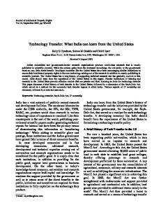
Cohort Effects vs. the Effects of Time in Low-Poverty Areas One source of bias in CM’s estimates is that they confound the effects on economic outcomes of spending more time in a low-poverty area with differences in program impacts that vary by randomization entry cohorts in MTO. Because of the limited capacity of the nonprofit agencies that helped MTO experimental families relocate, and for other reasons, families who enrolled in MTO were randomly assigned into different mobility groups over an extended period of time ranging from 1994 to 1998. CM’s key explanatory variables of interest are the number of months spent in low-poverty (! 20%) and high-poverty (≥ 20%) areas, both of which will on average be higher for earlier cohorts for mechanical reasons. In fact, the only reason CM are even able to estimate a model that controls for time in both low-poverty and high-poverty census tracts, yet avoids the problem of perfect multicollinearity, is that some families were randomly assigned earlier in time than others and so will have more months of address data available between the time of randomization and the interim MTO survey.20 CM’s estimates confound cohort differences in MTO impacts on survey outcomes with changes in impacts over time for reasons similar to those in demography that often make it hard to disentangle age, period, and cohort effects. Some evidence for cohort differences in MTO impacts comes from table 3, taken from Orr et al. (2003, table G-7), which shows TOT impacts on administrative data measures for TANF and food stamp benefits, taken five years after random assignment for cohorts randomly assigned earlier (with an average time between randomization and interim survey of 81

20 If all MTO families had the same amount of postrandomization data (the same number of months between time of random assignment and time at which the interim MTO survey was conducted), the explanatory variables for number of months in lowpoverty integrated, low-poverty segregated, and high-poverty census tracts would be perfectly multicollinear. This is easy to see by imagining that we simply rescaled the variables for time in low-poverty and high-poverty areas by dividing by the sample mean for total number of months of post–random assignment address data. If the amount of postrandomization data were the same for everyone (always equal to the mean), then the measures for share time in low-poverty and high-poverty areas would together sum to one.

171

American Journal of Sociology TABLE 3 Year 5 TOT Impacts on Outcomes Measured with Longitudinal Administrative Records (in dollars) Experimental Outcome TANF benefits . . . . . . . . . . Food stamp benefits . . . .

Early Cohort ⫺484 (251) ⫺421* (173)

Section 8

Late Cohort

Early Cohort

Late Cohort

617 (335) 464* (226)

⫺252 (218) 20 (153)

628* (236) 388* (178)

Source.—Orr et al. 2003, table G-7 (p. G-19). Notes.— Numbers in parentheses are SEs. Results reported in constant 2001 dollars (see Orr et al. 2003, p. 137). * P ! .05.

months) and those assigned later (average of 62 months).21 The TOT impacts are relatively large and negative for TANF and food stamp receipt for the early cohorts—MTO moves cause these cohorts to be less likely to be on social programs—but the impacts are large and of the opposite sign for the later cohorts. Since earlier cohorts seem to benefit more from MTO than later cohorts, CM’s estimates attribute some effect to extra time in low-poverty areas that is actually simply due to the fact that earlier MTO cohorts seem to benefit more from the program.22 CM’s model seems to load some of this cohort effect onto the coefficient estimates for time spent in both low-poverty and high-poverty areas. This helps explain why, in table 2, the coefficients on extra time spent in highpoverty areas are often a sizable share of the coefficients estimated for extra time in low-poverty integrated or segregated areas, and why the estimated coefficient for high-poverty areas is even different from zero at conventional statistical cutoffs for food stamp receipt. We can more directly see the confounding influences of cohort differences in MTO impacts by replicating CM’s model but now replacing their measure for number of months spent in high-poverty census tracts with a measure for the total number of months between random assignment 21

Orr et al. (2003, pp. G-18, G-19) note that random assignment occurred over an extended period of time, and some sites were faster than others in randomizing families. A simple split of the MTO sample by the calendar time in which families were randomly assigned would disproportionately assign families from some MTO sites to the “early cohort” group and other sites to the “late cohort” group, which would confound efforts to disentangle cohort differences from site differences in MTO impacts. As a result, Orr and colleagues split the sample roughly in half by time of random assignment within each site. 22 Orr et al. (2003, p. G-19) note there are several reasons why earlier cohorts might benefit more, including changes in HUD-funded demolitions of public housing over time that might have changed both the mix of families who enrolled in MTO and the neighborhood environments experienced by MTO controls.

172

MTO Symposium: What Can We Learn from MTO? in MTO and the interim MTO survey. Part D of table 2 shows that this measure for total months of postrandomization data available for each family, which is a direct indicator for which random-assignment cohort each MTO family belongs to, is statistically significant in each case and 1.5 to 2.0 times the estimated effect of extra time spent in a low-poverty segregated area. The estimated effect of time spent in low-poverty integrated neighborhoods is never statistically significant. The estimated effects of each extra month spent in a low-poverty segregated neighborhood are significant for three of CM’s economic outcomes, but the average marginal effects are quite small, equal to a 0.001 (one-tenth of a percentage point) increase in employment from each extra month in a low-poverty segregated census tract, a ⫺0.0009 change in TANF receipt, and ⫺0.001 for food stamp receipt.23 When we reestimate the model, pooling together months in low-poverty integrated and segregated tracts, we find no evidence for any statistically significant effect of extra time in low-poverty areas on any of the outcomes considered by CM. Selection Bias in Practice The results presented in table 2 suggest that there could be some modest correlation between time spent in a low-poverty neighborhood and economic outcomes, even after conditioning on cohort effects (by controlling for total months between random assignment and time of the interim survey). We believe that these correlations are susceptible to selection bias and so are wary of placing much inferential weight on CM’s findings or those in our own table 2. CM recognize that endogeneity or selection will necessarily be an issue with any nonexperimental analysis and so refer to their new estimates as “associations” rather than “effects.” At the same time, the title of CM’s article begins with “Neighborhood Effects,” not “Neighborhood Associations.” They claim that their analyses “provide strong evidence that neighborhoods may ‘matter’ in terms of adult economic self-sufficiency 23 Note that removing the variable for high-poverty months from the model means that time spent in these areas becomes the comparison group for the variables for time in low-poverty census tracts, and so we can then directly test the effect of time in high- vs. low-poverty areas using just the coefficients and standard errors for the lowpoverty measures. Part D of table 2 comes from using the NBER sample and NBER measures of low-poverty integrated and segregated neighborhoods but now replacing the measure of high-poverty neighborhood months with total months. When we use the CM sample and CM neighborhood measures and replace the measure for months in high-poverty areas with total number of post–random assignment months, we see a similar pattern, such that the estimated effect of time in low-poverty integrated areas is never statistically significant and time in low-poverty segregated tracts is significant for employment and food stamps.

173

American Journal of Sociology as well, though having more specific neighborhood targets and a longer required stay than MTO did are important. Thus, there is substantial evidence for keeping geographically specific vouchers on the table in order to offer low-income families a chance to improve their well-being” (pp. 139–40). CM are trying to thread a narrow rhetorical needle. They acknowledge that their estimates may be susceptible to some degree of selection bias, and so they do not want to claim that their new findings capture the precise causal effects of neighborhood environments on economic outcomes. But at the same time they want to argue that their new estimates provide enough useful information about neighborhood effects to inform policy decisions. What they seem to be implicitly claiming is that their estimates are, if not exactly right, at least in the right ballpark. However, there is no way to tell whether these results are in fact in the right ballpark. Recall that CM’s model includes measures of time spent in low-poverty neighborhoods and indicators for MTO treatment group and compliance status. CM’s estimates for the effects of specific neighborhood characteristics on economic outcomes are thus essentially a weighted average of three regression-adjusted differences: the mean outcomes for experimental-group compliers who chose (or were able) to spend a long time in low-poverty areas versus compliers who spent less time in low-poverty areas; the difference in outcomes between experimental noncompliers who spent a long time in low-poverty areas versus those who spent less time in low-poverty areas; and the difference in outcomes between control families who spent more time in low-poverty areas than other families in the control group. CM’s approach to estimating the effects of cumulative time spent in low-poverty areas on employment outcomes measured from the interim survey is particularly vulnerable to selection biases. For example, any number of chance circumstances that might lead quickly to an unusually good job situation (e.g., seeing a “help wanted” sign for a well-paying job in a neighborhood store) will increase the chances of being able to afford to continue to live in a better neighborhood and having a better job at the time of the interim survey. In this case, employment is as much a cause as a result of the neighborhood conditions. A growing body of research demonstrates that the magnitude of selection bias with nonexperimental estimators can often be quite large in practice. This type of evidence is derived from what Shadish (2000) calls a “within-study comparison,” which involves using data from a randomized experiment to estimate the true causal effect of some policy or program intervention and then reestimating the effect using different nonexperimental methods. In our own previous research, we have shown that applying nonexperimental estimates to the MTO data can lead to severely 174

MTO Symposium: What Can We Learn from MTO? biased estimates that are far away from the true causal effects estimated using the randomly assigned variation in the experimental data. For example, Kling et al. (2007, p. 98) use data just from the MTO control group alone and regress a measure of duration-weighted average census tract poverty against various outcomes, controlling for a similar set of baseline characteristics to that employed by CM. They find that ordinary least squares (OLS) estimates are typically of the opposite sign of those derived by using MTO random assignment as an instrument for tract poverty rates. Moreover, they suggest that the nature of the selection process is more complicated than is often assumed, because “adults and families with female teenagers likely to have adverse outcomes tended to move to low-poverty neighborhoods, and families with male teenagers likely to have beneficial outcomes tended to move to low-poverty neighborhoods” (Kling et al. 2007, p. 107). We have also found severe bias resulting from applying nonexperimental methods to the MTO data even in our study of violence among young people, for which we have detailed data about preprogram outcomes that are relatively strong predictors of subsequent behavior. Ludwig and Kling (2007) generate a nonexperimental estimate for the effect of neighborhood violent-crime rates on violent behavior by individual MTO program participants by using data just from the MTO experimental group alone. These nonexperimental estimates suggest that a 1-SD increase in the local-area violent crime rate leads to 0.078 more violentcrime arrests per male youth in the MTO study (SE p 0.046), even after controlling for the census-tract poverty rate and share minority. In contrast, experimental estimates that use data from all three MTO groups and interactions of MTO group assignment and demonstration site as instruments suggest no effect, or perhaps even the opposite relationship (point estimate of ⫺0.109; SE p 0.117). More generally, studies dating back at least to LaLonde (1986) yield an accumulating body of evidence that nonexperimental estimates can often be severely biased, even in cases where relatively rich covariate data are available. Even commonly used approaches to this problem, such as difference-in-differences and propensity-score methods, have been found to be subject to large biases in other applications such as job training programs or schooling (Agodini and Dynarski 2004; Wilde and Hollister 2007).24 In some cases, nonexperimental methods are able to come “close” 24 LaLonde (1986) focuses on estimating the effects of workforce training programs on less skilled workers, based on data from a randomized job-training experiment carried out by the Manpower Demonstration Research Corporation in the 1970s. A large follow-up literature has reexamined this issue in the job-training application, sometimes using the same data as LaLonde but otherwise often focusing on job training, in part because of the availability of experimental data in that area. For a recent discussion

175

American Journal of Sociology to the true causal effect revealed by experimental analysis, consistent with the idea that in some cases selection into different treatments or social settings could potentially occur mostly on the basis of individual characteristics that are observable to the analyst. The problem is that the diagnostic tools available for determining when a given nonexperimental method is working well in a given application are quite limited in their predictive power. Thus, we are wary of placing a great deal of inferential weight on the bulk of nonexperimental neighborhood effects study that dominates the literature. We believe that nonexperimental methods can sometimes be useful. But in our judgment, useful causal inferences are most likely to come from nonexperimental research designs that focus on understanding the process through which people are assigned or select into different programs or social environments. In particular, when selection is known to have occurred on the basis of observable characteristics, then some regression or propensity-score methods can yield useful evidence. More often, we do not know exactly what is driving the selection process, and we should worry that selection could occur in part on the basis of factors that are not well understood or easily measured. In these cases, valid causal inference is most likely to come from studies that can isolate aspects of the treatment process that are plausibly unrelated to individual characteristics that also affect outcomes and from using just the variation in treatments or social settings generated by that exogenous process—that is, focusing on the study of “natural experiments.” Good examples in the area of neighborhood or housing studies include Oreopoulos (2003), Jacob (2004), and Jacob and Ludwig (2007). CM take exactly the opposite approach—they ignore the exogenous variation in neighborhoods generated by MTO and focus entirely on the self-selected differences in neighborhoods within randomly assigned MTO groups—so there is no reason to put any stock in their results. Estimating Duration Impacts The longitudinal administrative data that were collected for the interim MTO evaluation provide some suggestive—but only suggestive—evifocused on the use of propensity-score methods in this application, see Dehejia and Wahba (1999), Michalopoulos, Bloom, and Hill (2004), and Smith and Todd (2005). More recently, Greenberg, Michalopoulos, and Robins (2006) use a “between-study comparison” and ask whether the nonexperimental literature on job training as a whole is consistent with the experimental literature overall, adjusting for differences across studies in things like program populations and job-training interventions. They find that the two types of research literatures are reasonably close with respect to jobtraining impacts on women, but not very close for men or adolescents.

176

MTO Symposium: What Can We Learn from MTO? dence that MTO’s impacts on adult economic outcomes might become more beneficial over time (Orr et al. 2003; Kling et al. 2007). An alternative approach to examining the effects of time spent in a low-poverty area that is more in keeping with MTO’s experimental design is to use the IV approach from Kling et al. (2007). This approach exploits the fact that the MTO experimental-group and Section 8 comparison-group treatments generate different effects on postrandomization neighborhood trajectories, and these treatment effects on neighborhood trajectories vary across MTO demonstration sites. This enables us to compare variation across sites in MTO group differences with respect to neighborhood characteristics with group differences in economic or other outcomes to test for a “doseresponse” relationship. For example, in every MTO demonstration site, average durationweighted tract poverty rates are lower for families assigned to the experimental group than for those in the control group. (This explanatory variable, unlike the one used by CM, is not mechanically related to the time at which families were randomly assigned). But these experimental/ control differences in average tract poverty rates vary across sites, as shown in figure 1, which presents mean adult employment rates and average tract poverty rates for each MTO group by site, relative to each site’s mean. Specifically, the experimental/control difference in average tract poverty rates is largest in the Los Angeles site, smallest in the Boston site, and roughly similar in magnitude in the other MTO demonstration sites. Figure 1 also demonstrates the value for tracing out these neighborhood effect dose-response relationships that is added by having data on a second mobility group—the Section 8 comparison group, which was offered unrestricted housing vouchers to relocate and in every site experienced changes in average tract poverty rates that are somewhat more modest than those experienced by the experimental group in that site. Note, for example, that the Section 8/control difference in average tract poverty rates is smallest in New York even though the experimental/ control difference in tract poverty for that site is not an outlier compared to the other sites. The differences across sites in MTO mobility-group variation in average tract poverty rate are due to some combination of MTO experimental or Section 8–only compliers’ making relatively more dramatic initial MTO moves in some sites than in others and/or their willingness to persist in low-poverty areas for longer periods of time. If adult employment outcomes were improved by greater exposure to relatively lower-poverty census tracts, then we would see the largest difference in adult employment rates (vertical axis) between the Los Angeles experimental and control groups (the site-groups with the largest difference in average tract poverty rate, as shown in the horizontal axis). But in fact, the average employment rates are very similar in the experimental 177

Fig. 1.—Mean adult employment rates and duration-weighted average tract poverty rates by MTO site and group, full sample. Sample is all MTO adults who responded to the interim survey. S p Section 8 comparison group; E p experimental group; C p control group. Results are calculated using weights that adjust for changes over the MTO study period in the probability of being assigned to the different MTO mobility groups. Each data point in the figure is the weighted mean employment rate from the interim survey for adults in the specified MTO group and demonstration site, minus that site’s mean employment rate, and the duration-weighted average census-tract poverty rate for adults in the specified MTO group and demonstration site, minus that site’s mean average tract poverty rate. The line shows a simple linear regression fit through the data points. Our IV estimates shown in table 3 are essentially equal to this regression line, although the formal IV results will be slightly different because they (unlike the line in fig. 1) also control for baseline covariates to improve the precision of the estimate.

MTO Symposium: What Can We Learn from MTO? and control groups in the Los Angeles site. The same dose-response logic suggests that we should see a relatively small difference in employment rates between the Section 8 and control groups in the New York site, since the group contrast in average tract poverty is smallest here compared to all of the other treatment/control contrasts across the MTO sites. But again, that is not the case. More generally, the regression line fit through the 15 site-group means shown in figure 1 is downward-sloping but rather flat, suggesting that there is not much relationship between average tract poverty rates and employment rates. This regression line through the site-group means is essentially what is estimated by a two-stage least squares procedure that uses interactions between indicators for MTO demonstration sites and mobility group assignments as instrumental variables for average tract poverty rate in a regression that has adult employment as the outcome of interest. With this approach, a neighborhood socioeconomic measure such as duration-weighted average tract poverty rates (POV) is viewed as a summary index for a bundle of neighborhood characteristics that are changed as a result of MTO. Interactions between treatment-group assignments (e) and site indicators (S) are used as instrumental variables to isolate the experimentally induced variation in POV across sites and groups, as in equation (1), where the main site effects are subsumed in X together with the same standard set of baseline covariates controlled for by CM and in our own previous published work on MTO. Controlling for these baseline covariates serves mainly to improve the precision of our estimates. We also use weights to adjust for changes over the course of the MTO experiment in the probability that subjects are randomly assigned to the three MTO mobility groups (see Orr et al. 2003). The first-stage power of our estimates is quite high: The F-test for the joint significance of the instruments in first-stage equation (1), using the full sample, is equal to 40.5 (P ! .001). Table 4 shows the results for l2 from a separate estimation of equations (1) and (2) for different outcomes and analytic samples, where Y in equation (2) is some behavioral outcome of interest. POV p (e # S)m1 ⫹ Xb1 ⫹ ␧1.

(1)

Y p POVl 2 ⫹ Xb2 ⫹ ␧2.

(2)

Table 4 shows the results of estimating this IV procedure for different outcome measures (rows) and analytic samples (columns), where each cell reports the coefficient from a different two-stage least squares regression. We do not see much support for the idea that more pronounced and sustained changes in tract poverty rates translate into improved adult 179

American Journal of Sociology TABLE 4 Instrumental Variable Estimates for Effects of Tract Poverty on MTO Adult Economic Outcomes

Outcome Measure

Full Sample

Psychological distress (K-6 index) . . . . . . . . . . . . . . . . . . . . . .239* (.117) Employed . . . . . . . . . . . . . . . . . . . ⫺.159 (.161) Weekly earnings . . . . . . . . . . . . 29 (71) TANF receipt . . . . . . . . . . . . . . . .147 (.151) Food stamps receipt . . . . . . . . .028 (.160) N ............................. 3,664

Random Cohort Assignment Early

Late

.112 (.174) ⫺.253 (.234) ⫺59 (106) .411 (.216) .290 (.238) 1,823

.284* (.142) ⫺.016 (.202) 164 (88) ⫺.150 (.195) ⫺.244 (.200) 1,841

Notes.—The table presents point estimates and SEs (in parentheses) using interactions of MTO treatment group and MTO demonstration site as instrumental variables for durationweighted postrandomization average tract poverty rate. These estimates control for a set of standard baseline covariates related to the adult’s educational attainment, baseline employment status, and social program participation and use weights to adjust for a change in the randomization rates across MTO groups during the course of the program period (see Orr et al. [2003] for details). * P ! .05.

economic outcomes. We see slightly larger point estimates for labor market outcomes for early cohorts relative to those derived using either the full sample or just the late cohorts, but this may simply reflect the fact that the economic outcomes for earlier cohorts of program participants respond differently than do those of later cohorts (as demonstrated in table 3). In contrast, the estimate in the top row of table 4 for the full MTO sample indicates a large and statistically significant improvement in adult mental health (reductions in Ronald Kessler’s K-6 index) from more time spent in lower-poverty areas. It is important to note that our IV estimates in table 4 cannot be interpreted literally as the effects of changing neighborhood poverty rates on the economic outcomes of MTO adults. Our tract poverty measure captures the effects of the entire bundle of community attributes that are correlated with tract poverty and that influence economic outcomes. With only 10 instruments, our ability to isolate the distinct effects of separate neighborhood attributes on outcomes is necessarily limited (see Kling et al. [2007] for an extended discussion).25 25 Ludwig and Kling (2007) show that there is enough variation across MTO sites and groups to distinguish the effects of tract SES composition from tract racial composition on violent-crime arrests of MTO participants. When we try to instrument for both tract SES and racial composition with adult economic outcomes as the dependent variable of interest, the estimated effects of duration-weighted tract poverty change only slightly in comparison to the results in table 4, while the estimated effects for tract share minority are quite imprecise.

180

MTO Symposium: What Can We Learn from MTO? CONCLUSIONS

Empirical evidence on the existence and nature of neighborhood effects is important, given that fully 7.9 million people lived in high-poverty census tracts in 2000 (Jargowsky 2003). Housing and other social policies affect the concentration of poor families in highly disadvantaged neighborhoods. There is great demand from policy makers across the country to understand whether and how neighborhood environments affect the life chances of low-income families, and, if so, what to do about it. The MTO experiment provides the best opportunity to date for answering some of these questions. Our disagreement with CM concerns the best way to analyze the MTO data and what inferences can and cannot be supported from these analyses. CM end their article with an argument for how analysts should use the MTO data in the future: “Measuring the effect of a voucher offer is vital to assessing the experimentally sound results of the policy demonstration. However, if MTO data are used to measure neighborhood effects, different assumptions and techniques should be considered,” using nonexperimental models that “sacrifice MTO’s experimental design” (p. 139). We believe that their assessment of the ability of experimental MTO analysis to be informative about neighborhood effects is misguided and that their specific prescriptions for future MTO analyses are likely to generate erroneous conclusions. Experimental estimates of the effects of MTO voucher offers and utilization are useful for understanding the scope of neighborhood effects on behavioral outcomes for low-income families, currently living in some of our nation’s most disadvantaged communities, who wish to relocate— a highly policy-relevant group. Random assignment of families to different MTO mobility groups, some of which are offered housing vouchers, generates large differences in average neighborhood trajectories across groups with respect to such community attributes as socioeconomic composition, safety, disorder, informal social control, and the social ties of MTO families themselves. Sociological and other theories predict that these neighborhood attributes influence behavior. Large neighborhood differences across MTO groups persist despite the fact that only some families assigned to the experimental group moved through the program, MTO moves generated relatively little residential integration by race and ethnicity, and some families moving in conjunction with the program eventually moved on to worse neighborhoods. None of these facts bias our ITT or TOT estimates of the effects of the differing neighborhood bundles caused by random assignment to the MTO treatment. If neighborhood environments affect behavior four to seven years after baseline among the sort of people who enroll in MTO, then these 181

American Journal of Sociology neighborhood effects ought to be reflected in ITT and TOT impacts on behavior. Thus, MTO tells us something important about the effects of mobility interventions in the medium run for an important population of lowincome families living in very distressed urban areas. It shows us that moving out of a disadvantaged, dangerous neighborhood into more affluent and safer areas does not have detectable impacts on economic outcomes four to seven years out. However, such neighborhood moves do have important effects on other self-reported measures of the wellbeing of program participants (which surely count for something), on adult mental health and some physical health outcomes, and on violent behavior among young people. Nonexperimental analyses of the type conducted by CM reintroduce all of the selection bias problems that MTO was designed to overcome. Moreover, their model confounds changes in neighborhood effects as families stay in low-poverty areas longer with neighborhood effects that vary by random assignment cohort in MTO, as suggested by the fact that controlling for random-assignment cohort greatly reduces the magnitude of CM’s estimated effects of time spent in low-poverty areas. And their results provide no support for their arguments about the importance of integrating by both race and social class. We should emphasize that the MTO estimates are informative only about the effects of mobility programs like MTO on the types of lowincome families who would choose to participate in such programs. MTO is silent on the effects of involuntary mobility programs, which is an important point, given ongoing HOPE VI activities across the country to demolish some of our highest-poverty housing projects. Readers are also cautioned against trying to draw inferences from MTO about interventions designed to change disadvantaged neighborhoods themselves, rather than relocating residents to other areas. Compared with MTO, this type of intervention requires much greater knowledge on the part of policy makers about what specific neighborhood attributes matter most for improving outcomes. If policy makers focus on changing the wrong set of neighborhood attributes, the impacts of a place-based intervention could be less beneficial than what we see in MTO. The effects of a place-based program might also differ from MTO because the former might be less disruptive to the existing social networks of families. Whether that would lead to more- or less-beneficial impacts compared to MTO is not obvious as a conceptual matter; for some families, existing social ties may hinder rather than help their economic and other outcomes, and so the net effect of leaving these networks unchanged will depend in part on the distribution of positive and negative network connections. We agree with CM that it is possible that MTO impacts on participating 182

MTO Symposium: What Can We Learn from MTO? families might grow larger over time, if families become more socially integrated into their new communities or are able to accumulate more human capital as a result of their improved mental health. The best way to test this hypothesis is additional data collection—from administrative records on MTO families for a longer time period and a second wave of detailed survey reports from MTO participants. This possibility suggests the great importance of continuing to follow MTO families into the future, a point that CM are sure to join our team in endorsing. APPENDIX

To help clarify the issues around selection bias, we review Heckman’s (1996) framework for thinking about how randomized experiments help overcome selection. Let Y1i represent some economic, health, or other outcome for a given low-income adult (i) if he uses a voucher to move into a low-poverty area, and let Y0i represent the outcome this person would receive if he did not have a voucher and so remained in a high-poverty area. Let di p 1 if the person uses a voucher; otherwise, di p 0. The essential problem for social scientists is that a given individual either uses a voucher or does not; we cannot observe both Y1i and Y0i at the same point in time for the same person, and so we must rely on different statistical methods to estimate the missing data on counterfactual outcomes. Assume that the potential outcomes for people in both states (low poverty with voucher and high poverty) are functions of observable variables (Xi) as well as other variables that are usually not observed in the standard data sets that are typically used to estimate neighborhood effects on labor market or other outcomes (Ui): Y1i p g1(Xi ) ⫹ U1i , E(U1i ) p 0;

(A1)

Y0i p g0 (Xi ) ⫹ U0i , E(U0i ) p 0.

(A2)

The outcome we actually observe for a given person is Yi p diY1i ⫹ (1 ⫺ di )Y0i, and so by substituting this into equations (A1) and (A2) and defining D i p (Y1i ⫺ Y0i ), we get Yi p g0 (Xi ) ⫹ di {[g1(Xi ) ⫺ g0 (Xi )] ⫹ (U1i ⫺ U0i )} ⫹ U0i p g0 (Xi ) ⫹ di D i ⫹ U0i .

(A3)

People might benefit from living in a lower-poverty neighborhood with a housing voucher because, for instance, labor market outcomes for high school dropouts (an observable characteristic in Xi) are better in areas 183

American Journal of Sociology that are closer to less-skilled job opportunities; this would be represented by the difference g1(Xi ) ⫺ g0 (Xi ). Alternatively, they might have improved labor market outcomes because living in a lower-poverty area reduces an unobserved variable that makes it difficult to work, such as stress; this would be reflected by the difference U1i ⫺ U0i. Equation (A3) is essentially a stylized version of the sort of nonexperimental regression analysis that dominates the neighborhood effects literature. Instead of a simple dichotomous indicator for living in a lowpoverty or high-poverty area, most studies regress some outcome of interest against a series of neighborhood variables that tend to be those that are easily measured from the decennial census, such as census-tract poverty rates or tract %minority. The key econometric issues are similar if d is a vector of continuous neighborhood measures rather than a binary scalar. The set of control variables (X) generally includes standard demographic variables such as age, education, and race and may also include more involved individual-level background variables, such as parents’ education levels, family income, or even more detailed measures of family functioning. Selection bias occurs when di is not orthogonal to the unobserved factors that influence outcomes (U1i and U0i in the equations above), so that E[U1i ⫺ U0iFdi p 1, Xi ] ( 0. Selection bias is difficult to avoid with nonexperimental analysis, because individual characteristics that affect the outcome variable will inevitably be left out of the regression. Moreover, the direction of this bias is difficult to predict by theory alone. Randomization solves the selection problem by causing the variation in neighborhood of residence to occur for reasons that are uncorrelated with individuals’ potential outcomes. Building on the notation introduced above, let ei p 1 if a person (i) is randomly assigned to the MTO treatment group and so is eligible to receive a MTO voucher, while ei p 0 if the person is assigned to the MTO control group. The main experimental results come from comparing the outcomes of all of the families randomized into the treatment group with those of all the families randomized into the control group, calculated mechanically by regressing Y against e and adjusting for baseline covariates X to improve precision. This ITT analysis measures the effect of offering families a housing voucher and housing mobility counseling. To see why partial compliance does not introduce selection bias in the experiment, use the potential outcomes framework from above and let P(di p 1FXi ) represent the probability that someone with observable characteristics Xi makes an MTO move in equation (A4). If MTO treatmentgroup assignment has no effect on those who do not move through the program (represented as E[YFd i i p 0, ei p 1] p E[YFd i i p 0, ei p 0]), then the change in outcomes (Y) induced by assignment to the experimental 184

MTO Symposium: What Can We Learn from MTO? rather than the control group is equal to the mean effect of MTO moves on those who move (represented as E(D iFdi p 1, Xi ), and known more generally as the TOT effect), multiplied by the share of people who will make MTO moves if given the chance, P(di p 1FXi ). Yi p g0 (Xi ) ⫹ [E(D iFdi p 1, Xi )]P(di p 1FXi )ei ⫹ (U1i ⫺ U0i )P(di p 1FXi )ei ⫹ U0i .

(A4)

The key virtue of random assignment is that the indicator for assignment to the treatment group, e, will be independent of the background characteristics of MTO sample respondents, X, the potential outcomes people would experience with and without a voucher, Y0 and Y1, and the probability of leasing up if offered a voucher, P(d p 1FX). The fact that only some MTO families assigned to the experimental group comply with their treatment assignment and relocate through the program does not introduce any bias to our estimates, because this propensity to move through MTO is balanced across families assigned to both the experimental and control groups. Similarly, random assignment balances the propensity to stay in a low-poverty area rather than move back to a slightly higher-poverty area, and so subsequent mobility after families make their initial MTO moves also does not introduce any bias to the ITT estimate. A more subtle point is that there is some “selection bias” in equation (A4), in the sense that the baseline covariates, X, are not independent of the unobserved determinants of potential outcomes U1 and U0 (Heckman 1996). In our previous published estimates for MTO impacts on outcomes (e.g., Kling et al. 2005; Kling et al. 2007), we controlled for baseline characteristics to improve the precision of our ITT and TOT estimates, but the fact that these baseline measures may be correlated with unobservable determinants of postrandomization outcomes means that we cannot interpret the coefficients on the baseline covariates as causal effects. But, as Heckman (1996) notes, this type of “selection bias” (correlation of background controls with the error term) is balanced across randomly assigned groups, and so it will not affect our ability to generate an unbiased ITT estimate. The ITT estimate compares all members of the treatment group to all members of the control group, and so by construction does not suffer from selection bias itself. REFERENCES Aber, J. Lawrence, Jeanne Brooks-Gunn, and Greg J. Duncan, eds. 1997. Neighborhood Poverty: Context and Consequences for Children, vols. 1 and 2. New York: Russell Sage Foundation. Agodini, Roberto, and Mark Dynarski. 2004. “Are Experiments the Only Option? A

185

American Journal of Sociology Look at Dropout Prevention Programs.” Review of Economics and Statistics 86 (1): 180–94. Bartus, Tamas. 2005. “Estimation of Marginal Effects using margeff.” Manuscript. http: //www.bke.hu/bartus/pdf/bartus_2005_sj.pdf Bloom, Howard S. 1984. “Accounting for No-Shows in Experimental Evaluation Designs.” Evaluation Review 8 (April): 225–46. Bloom, Howard S., et al. 1996. “The Benefits and Costs of JTPA Title II-A Programs.” Journal of Human Resources 12 (3): 549–76. Chamberlain, Gary. 1984. “Panel Data.” Pp. 1247–1320 in Handbook of Econometrics, vol. 2. Edited by Zvi Griliches and Michael D. Intriligator. Amsterdam: NorthHolland. Clampet-Lundquist, Susan, and Douglas S. Massey. 2008. “Neighborhood Effects on Economic Self-Sufficiency: A Reconsideration of the Moving to Opportunity Experiment.” American Journal of Sociology 114 (1): 107–43. Dehejia, Rajeev, and Sadek Wahba. 1999. “Causal Effects in Non-experimental Studies: Re-evaluating the Evaluation of Training Programs.” Journal of the American Statistical Association 94 (448): 1053–62. Ellen, Ingrid Gould, and Margery Austin Turner. 2003. “Do Neighborhoods Matter and Why?” Pp. 313–38 in Choosing a Better Life? Evaluating the Moving to Opportunity Social Experiment, edited by John Goering and Judith D. Feins. Washington, D.C.: Urban Institute Press. Glaeser, Edward L., Bruce Sacerdote, and Jose A. Scheinkman. 1996. “Crime and Social Interactions.” Quarterly Journal of Economics 111 (2): 507–48. ———. 2003. “The Social Multiplier.” Journal of the European Economic Association 1 (2–3): 345–53. Goering, John, Judith D. Feins, and Todd M. Richardson. 2003. “What Have We Learned about Housing Policy and Poverty Deconcentration?” Pp. 3–36 in Choosing a Better Life: Evaluating the Moving to Opportunity Social Experiment, edited by John Goering and Judith D. Feins. Washington, D.C.: Urban Institute Press. Greenberg, David H., Charles Michalopoulos, and Philip K. Robins. 2006. “Do Experimental and Nonexperimental Evaluations Give Different Answers about the Effectiveness of Government-Funded Training Programs?” Journal of Policy Analysis and Management 25 (3): 523–52. Heckman, James J. 1996. “Randomization as an Instrumental Variable.” Review of Economics and Statistics 78 (2): 336–41. Jacob, Brian A. 2004. “Public Housing, Housing Vouchers and Student Achievement: Evidence from Public Housing Demolitions in Chicago.” American Economic Review 94 (1): 233–58. Jacob, Brian A., and Jens Ludwig. 2007. “The Effects of Housing Vouchers on Children’s Outcomes.” Working paper. University of Michigan, Ford School of Public Policy. Jargowsky, Paul A. 2003. “Stunning Progress, Hidden Problems: The Dramatic Decline of Concentrated Poverty in the 1990s.” Policy brief. Brookings Institution, Washington, D.C. Jencks, Christopher, and Susan E. Mayer. 1990. “The Social Consequences of Growing Up in a Poor Neighborhood.” Pp. 111–86 in Inner-City Poverty in the United States, edited by L. E. Lynn, Jr. and M. G. H. McGeary. Washington, D.C.: National Academies Press. Kain, John F. 1968. “Housing Segregation, Negro Employment and Metropolitan Decentralization.” Quarterly Journal of Economics 82 (2): 175–97. Katz, Lawrence F., Jeffrey R. Kling, and Jeffrey B. Liebman. 2001. “Moving to Opportunity in Boston: Early Results of a Randomized Mobility Experiment.” Quarterly Journal of Economics 116:607–54. Keels, Micere, Stefanie DeLuca, Greg J. Duncan, Ruby Mendenhall, and James

186

MTO Symposium: What Can We Learn from MTO? Rosenbaum. 2005. “Fifteen Years Later: Can Residential Mobility Programs Provide a Long-Term Escape from Neighborhood Segregation, Crime, and Poverty?” Demography 42 (1): 51–73. Kling, Jeffrey R., Jeffrey B. Liebman, and Lawrence F. Katz. 2007. “Experimental Analysis of Neighborhood Effects.” Econometrica 75 (1): 83–119. Kling, Jeffrey R., Jens Ludwig, and Lawrence F. Katz. 2005. “Neighborhood Effects on Crime for Female and Male Youth: Evidence from a Randomized Housing Voucher Experiment.” Quarterly Journal of Economics 120 (1): 87–130. LaLonde, Robert J. 1986. “Evaluating the Econometric Evaluations of Training Programs with Experimental Data.” American Economic Review 76:604–20. Leventhal, Tama, and Jeanne Brooks-Gunn. 2000. “The Neighborhoods They Live In: The Effects of Neighborhood Residence on Child and Adolescent Outcomes.” Psychological Bulletin 126 (2): 309–37. Ludwig, Jens, Greg J. Duncan, and Paul Hirschfield. 2001. “Urban Poverty and Juvenile Crime: Evidence from a Randomized Housing-Mobility Experiment.” Quarterly Journal of Economics 116 (2): 655–80. Ludwig, Jens, Greg J. Duncan, and Joshua C. Pinkston. 2005. “Housing Mobility Programs and Economic Self-Sufficiency: Evidence from a Randomized Experiment.” Journal of Public Economics 89 (1): 131–56. Ludwig, Jens, and Jeffrey R. Kling. 2007. “Is Crime Contagious?” Journal of Law and Economics 50 (3): 491–518. Ludwig, Jens, Helen Ladd, and Greg J. Duncan. 2001. “The Effects of Urban Poverty on Educational Outcomes: Evidence from a Randomized Experiment.” Pp. 147–201 in Urban Poverty and Educational Outcomes, edited by William Gale and Janet Rothenberg Pack. Brookings-Wharton Papers on Urban Affairs. Washington, D.C.: Brookings Institution Press. Luttmer, Erzo F. P. 2005. “Neighbors as Negatives: Relative Earnings and Well-Being.” Quarterly Journal of Economics 120 (3): 963–1002. Matthews, Jay. 2007. “Neighborhoods’ Effect on Grades Challenged: Moving Students Out of Poor Inner Cities Yields Little, Studies of HUD Vouchers Say.” Washington Post, August 14. Page A2. Mendenhall, Ruby, Stefanie DeLuca, and Greg Duncan. 2006. “Neighborhood Resources, Racial Segregation and Economic Mobility: Results from the Gautreaux Program.” Social Science Research 35 (4): 892–923. Michalopoulos, Charles, Howard S. Bloom, and Carolyn J. Hill. 2004. “Can Propensity Score Methods Match the Findings from a Random Assignment Evaluation of Mandatory Welfare-to-Work Programs?” Review of Economics and Statistics 86: 156–79. Moffitt, Robert A., ed. 2003. Means-Tested Transfer Programs in the United States. Chicago: University of Chicago Press. Newhouse, Joseph P., and IEG (the Insurance Experiment Group). 1993. Free for All? Lessons from the RAND Health Experiment. Cambridge, Mass.: Harvard University Press. Oreopoulos, Philip. 2003. “The Long-Run Consequences of Growing Up in a Poor Neighborhood.” Quarterly Journal of Economics 118 (4): 1533–75. Orr, Larry L., Howard S. Bloom, Stephen H. Bell, Fred Doolittle, Winston Lin, and George Cave. 1996. Does Training for the Disadvantaged Work? Evidence from the National JTPA Study. Washington, D.C.: Urban Institute Press. Orr, Larry L., Judith D. Feins, Robin Jacob, Erik Beecroft, Lisa Sanbonmatsu, Lawrence F. Katz, Jeffrey B. Liebman, and Jeffrey R. Kling. 2003. Moving to Opportunity Interim Impacts Evaluation. Washington, D.C.: U.S. Department of Housing and Urban Development, Office of Policy Development and Research. Rosenbaum, James E. 1995. “Changing the Geography of Opportunity by Expanding

187

American Journal of Sociology Residential Choice: Lessons from the Gautreaux Program.” Housing Policy Debate 6 (1): 231–69. Rubin, Donald B. 1980. “Comment on ‘Randomization Analysis of Experimental Data: The Fisher Randomization Test,’ by D. Basu.” Journal of the American Statistical Association 75:591–93. Rubinowitz, Leonard S., and James E. Rosenbaum. 2000. Crossing the Class and Color Lines: From Public Housing to White Suburbia. Chicago: University of Chicago Press. Sampson, Robert J., Jeffrey D. Morenoff, and Thomas Gannon-Rowley. 2002. “Assessing ‘Neighborhood Effects’: Social Processes and New Directions in Research.” Annual Review of Sociology 28:443–78. Sampson, Robert J., Stephen W. Raudenbush, and Felton Earls. 1997. “Neighborhoods and Violent Crime: A Multilevel Study of Collective Efficacy.” Science 277 (5328): 918–24. Sanbonmatsu, Lisa, Jeffrey R. Kling, Greg J. Duncan, and Jeanne Brooks-Gunn. 2006. “Neighborhoods and Academic Achievement: Results from the Moving to Opportunity Experiment.” Journal of Human Resources 41 (4): 649–691. Shadish, W. R. 2000. “The Empirical Program of Quasi-experimentation.” Pp. 13–36 in Research Design: Donald Campbell’s Legacy, edited by L. Bickman. Thousand Oaks, Calif.: Sage. Shroder, M. 2002. “Locational Constraint, Housing Counseling, and Successful LeaseUp in a Randomized Housing Voucher Experiment.” Journal of Urban Economics 51:315–38. Smith, Jeffrey, and Petra Todd. 2005. “Does Matching Overcome LaLonde’s Critique of Non-experimental Estimators?” Journal of Econometrics 125:305–53. Sobel, Michael E. 2006. “What Do Randomized Studies of Housing Mobility Demonstrate? Causal Inference in the Face of Interference.” Journal of the American Statistical Association 101 (476): 1398–1407. Solon, Gary, Marianne E. Page, and Greg J. Duncan. 2000. “Correlations between Neighboring Children in their Subsequent Educational Attainment.” Review of Economics and Statistics 82 (3): 383–92. Turney, Kristin, Susan Clampet-Lundquist, Kathryn Edin, Jeffrey R. Kling, and Greg J. Duncan. 2006. “Neighborhood Effects on Barriers to Employment: Results from a Randomized Housing Mobility Experiment in Baltimore.” Pp. 137–87 in Brookings-Wharton Papers on Urban Affairs, edited by Gary Burtless and Janet R. Pack. Washington, D.C.: Brookings Institution Press. Votruba, Mark E., and Jeffrey R. Kling. 2004. “Effects of Neighborhood Characteristics on the Mortality of Black Male Youth: Evidence from Gautreaux.” Working paper no. 491. Princeton University, Industrial Relations Section. Wilde, Elizabeth Ty, and Robinson Hollister. 2007. “How Close is Close Enough? Evaluating Propensity Score Matching Using Data from a Class Size Reduction Experiment.” Journal of Policy Analysis and Management 26 (3): 455–78. Wilson, William Julius. 1987. The Truly Disadvantaged: The Inner City, the Underclass, and Public Policy. Chicago: University of Chicago Press.

188