Wetting and spreading phenomena Ponnuraj Krishnakumar May 13, 2010
Abstract Understanding wetting phenomena involves a careful and detailed study of the various surface tension forces, fluctuations and other contact line dynamics. Cahn’s phenomenological theory combines the effects of short-range and some long-range forces to produce a phase diagram and the two critical exponents that characterize behavior near Tc . Experiments in the past two decades have been able to test and verify the phase diagram predicted in Cahn’s theory. Further the critical exponents obtained in experiment closely agree with those obtained in theory. All of the theory and the results are presented here.
1
I. Introduction Whenever a drop of liquid is placed on the surface of a substrate, the liquid is expected to evolve until it reaches an equilibrium state. This may require the drop to either spread and cover the surface or remain as a drop or in some cases even try to leave the surface. Such a process depends on properties of the surfaces involved as well as the external conditions such as temperature. This field is broadly categorized as wetting and spreading phenomena and aims to determine how a liquid behaves on the surface of a substrate. Wetting phenomena are widespread in nature and occur whenever a surface is exposed to an environment. Understanding why and when a liquid decides to wet a surface can greatly improve our knowledge of everyday events. Further, this information can help in designing new materials and technology. This review is aimed at providing a basic analysis of wetting and the different phase transitions that arise during the process. The topics presented here are directly related to the material covered in phase transitions course during the semester and ties concepts of discontinuous and continuous phase transitions, and critical exponents to an excellent real life scenario. Further, this is also a topic of current and growing interest for both theorists and experimentalists. New developments and recent experiments are constantly improving our understanding in this field. Section 2 of this paper introduces the basic concepts of surface wetting, drop spreading, the different phases involved and some of the details involved in the study of surface wetting. In general wetting characteristics are quite complex and require a very detailed analysis. This review is restricted to explaining wetting phenomena in ideal equilibrium situations and providing a theory that qualitatively explains the process. Section 3 focuses on the near equilibrium state of a liquid deposited on the surface of another liquid or solid. This section includes a model based on the intermolecular forces and a phenomenological theory proposed by Cahn. From Cahn’s theory, one can obtain a phase diagram that describes the various phase transitions between a wetting, dewetting and a partial wetting phase. Most of the major theories introduced are followed by experimental data that test the theoretical predictions.
2. Basics of wetting and spreading 2.1 Surface thermodynamics When considering a liquid on a surface, there are three systems that come into play; the liquid, the surface and the surrounding atmosphere which is referred to as the vapor. The relation between the various surface tensions and the contact angle was given by Young [13] in Eq. 1 γSV = γSL + γLV cosθeq
(1)
Here S, V and L refer to the substrates surface, the vapor and the liquid respectively. θ is the contact angle as shown in Figure 1. Young’s equation in the 2
above form describes the equilibrium situation when the surface tension forces balance each other.
Figure 1: Young’s equation equates the surface tension forces at equilibrium For a given set of surfaces, the corresponding θeq can be obtained from the surface tensions involved. If, for instance γSV = γSL + γLV , then θeq = 0 and equilibrium corresponds to when the liquid is spread across the surface of the substrate. This situation is referred to as wetting. The other two phases that arise are the dewetting phase and the partial wetting phase. Though in practice dewetting is rare, from a thermodynamic point of view both wetting and dewetting are similar under exchange of surface and the vapor systems. Thus, it suffices to consider and study the wetting state, which is characterized by a macroscopically thick layer. In the partial wetting state, the drops on a surface are surrounded by a microscopically thin film adsorbed at the surface. The three wetting states are shown in Figure 2. In typical experiments film thickness may range from a molecule to several molecules.
Figure 2: The three different wetting phases One can define an equilibrium spreading coefficient Seq to help classify the different wetting states. Seq ≡ γSV − (γSL + γLV ) = γLV (cosθeq − 1)
(2)
Seq above measures the difference between the surface free energy γSV and its value in the case of complete wetting. Notice that in general Seq ≤ 0 and Seq = 0 only in the case of complete wetting. When a drop of liquid first encounters a surface, it is far from the equilibrium state. An initial spreading coefficient may be defined as follows [4] Si = γS0 − (γSL + γLV ) 3
(3)
Figure 3: The radius R as a function of time as given by Tanner’s law. where γS0 is the surface tension of the dry solid substrate. If Si < 0, the drop will have a finite contact angle θi and prefer to remain in a partial wetting state. On the other hand, if Si > 0 the drop will tend to spread out and wet the surface. An analysis of the adsorption equation shows that in general Si > Seq . This implies, whenever Si < 0, this ensures that Seq < 0. Nothing definite can be said about the sign of Seq , if Si > 0. 2.2 Drop spreading This part covers some basics of drop spreading. As discussed above, when a drop is generally placed on a surface, it is far from equilibrium (Si 6= Seq ). Consider the simple case of a small viscous droplet on a surface. Here small implies that the drop radius is less than the capillary length lc , given by [1] p (4) lc = γ/ρg The capillary number gives the ratio of the viscous and surface tension forces. Ca = U η/γ
(5)
Ca ≈ 10−5 − 10−3 in most spreading experiments, η is the liquid viscosity and 0 U = R is the contact line speed. Combining these results one can obtain a relationship between drop radius and time as give by Tanner’s law (Eq. 6) [12] and shown in Figure 3. "
10γ R(t) ≈ 9Bη
�
4V π
�3 #1/10
∝ tn
(6)
The rate at which a drop spreads is determined by the interplay between the surface energies, gravity and dissipation. For small drops the surface free energy also plays a role [1]. Fs = 4V 2 γ/πR4 − πSi R2 4
(7)
The first term in this expression corresponds to the liquid-vapor interface due to the curved nature of the drop and the second term arises due the base area of the drop being covered by fluid. By inspection of the above equation, it appears that when Si > 0, spreading would lead to a reduction in the surface free energy. However, in practice this reduction in free energy is not always converted to macroscopic motion of the drop. Instead only some of the molecules near the contact line may spread out creating a sort of thin precursor film around the drop. This process uses up the energy that could have gone toward spreading the entire drop. As Fs reduces, the effective radius R still increases. This causes spreading coefficient to approach an equilibrium value slowing down the rate of spreading. In order to compute the power n in Tanner’s equation (Eq. 6), one has to measure the rate of energy dissipation near the contact line. So far our analysis has concentrated on drops of small radius which lead to Tanner’s law. However, as the radius grows, the assumption that it is much less than the capillary length is invalid. The drop now resembles a pancake of uniform thickness with curves just at the rims. The main driving force now is gravity and when balanced against dissipation near the contact line one obtains the critical exponent in R ∝ tn as n = 1/7 or n = 1/8. The exponent n obtained from various procedures is tabulated in Figure 4.
Figure 4: Scaling exponents n, for R ∝ tn as obtained from different theories and corresponding experiments [1]
3. Equilibrium wetting phenomena Section 2 introduced the basic idea behind surface wetting and how a drop of liquid is expected to spread as given by Tanner’s Law. The current section concentrates on wetting under equilibrium conditions. 3.1 Long-range intermolecular forces The cohesive interactions between the surfaces are considered and approximated in the form of a molecular interaction potential. Israelachvili [5] showed that molecular interaction potentials with a short range repulsion and an algebraically decaying attraction assumes the Lennard-Jones form 5
w(r) = 4�[ρ/r
12
6
− ρ/r ]
(8)
Although the above expression describes the London dispersion energy between non polar molecules as well as the Debye energy between molecules, there are other short range forces that lead to exponential decay. These short ranged forces are called polar and the forces causing the algebraic decay (1/r6 ) potentials as apolar. To quantify the net effect of the interaction potential on wetting behavior, consider a liquid film of thickness l on a solid substrate. If the adhesive interactions are strong, the system can lower its free energy by increasing the distance between two surfaces. This leads to a net repulsive force per unit area between the solid-liquid and liquid-vapor interfaces, which is called the disjoinQ ing pressure (l) and can be measured in experiment. The relation between the disjoining pressure and the interface potential V (l) is Y (l) = −dV (l)/dl (9) where γSV (l) = γLV + γSL + V (l)
(10)
is the excess free energy per unit area of the liquid film. In the case Si > 0, the static film thickness is governed by minimizing the surface free energy (not V (l)). This leads to the condition [3] [V (l) − V (0)]/l = dV (l)/dl
(11)
Such a drop would prefer to spread across the entire substrate but is restricted by its finite volume. As a compromise is assumes a pancake like shape. In principle the equilibrium state can be predicted from the disjoining pressure, but such a calculation is difficult. Another method is to perform numerical calculations (such as DFT) of the Lennard-Jones potentials. DFT calculations of simple atoms or molecules have also been verified by experiment. There are many subtleties involved in DFT calculations of more complex systems. The second term in Eq. 8 includes all types of intermolecular dipole interactions. Israelachvili [5] showed that the decay Y (l) ≈ A/6πl3 (12) where A is called the Hamaker constant. The Hamaker constant plays an important role in determining which phase the liquid will assume on the surface. To see this more clearly, consider the relation: Z ∞ Y Seq = (l)dl (13) lmin
If Seq < 0, this leads to partial wetting irrespective of Hamaker’s constant A. On the other hand, when Seq = 0 and A > 0, this leads to the formation of a wetting layer. Other intermediate states arise for other values of Seq and A. 6
Further, the Hamaker constant can easily be obtained from the dielectric properties of the materials and thus is measurable in experiment. 3.2 Short-range forces: Cahn-Landau phenomenological theory of wetting Cahn proposed a phenomenological theory of surface free energy along with a Landau expansion [2], in order to explicitly calculate Seq . Cahn’s theory can be used to determine wetting phase transitions when short-range forces are involved. It can also be adapted to include some long range interactions such as the van der Waals forces as shown in section 3.4. The free energy as introduced by Cahn is Z x [(c2 /4)(dm/dz)2 + ω(m)]dz (14) Fs = Φ(ms ) + 0
where ω is the bulk free energy, m(z) is the order parameter as a function of distance from the substrate. The term Φ(ms ) was included by Cahn to account for the solid surface and can be expanded as [6] Φ(ms ) = −h1 ms − gm2s /2
(15)
Here h1 is the short-range surface field and g is the surface enhancement. The field h1 depends on the surface tensions between the surfaces and determines whether a liquid or vapor state is preferred. If h1 < 0, the vapor state is favored and if h1 > 0, liquid state is preferred. The surface enhancement factor g accounts for fact that molecules on the boundary have fewer interactions due to lesser neighbors. The 3D phase diagram obtained from Cahn-Landau theory by Nakanishi and M. Fisher [6] is shown in Figure 5.
Figure 5: Wetting phase diagram obtained from Cahn-Landau theory. The curve W repre1 sents the wetting line with the critical temperature Tc at its apex. The tricritical point Tw separates the first-order transition and second-order transition realms. [6]
The three axes are the bulk field h, the reduced temperature t, and the surface field h1 . The surface field, h ≡ (µ − µ0 )/kB T , measures the distance in 7
terms of a bulk chemical potential from two-phase coexistence. For large values of h1 the transition is 1st order. However, as one reduces h1 below the Tw1 tricritical point, the phase transition becomes 2nd order. These transitions and the triciritical points have been observed experimentally showing that the CahnLandau theory serves as a good tool to understanding wetting transitions. These results are shown in section 3.3. DFT simulations have also produced similar results. Complete wetting is more likely to occur at higher temperatures. In the first-order transition region this corresponds to a discontinuous jump from a thin film to an infinitely thick film i.e the potential V (l) is minimum for thin films at low T and for thick films at high T . For the case of continuous phase transition, there is a gradual shift in the minimum to an infinitely thick film. Two independent exponents characterize the critical behavior of a wetting transition. The first comes from analyzing how cosθeq approaches 1 (θeq → 0) at the wetting transition. This is directly related to the surface specific heat which has the form given by the below relation. (1 − cosθeq ) ∝ (Tw − T )2−αs
(16)
For αs = 1, the first derivative of γSV is discontinuous and the transition is first-order. However, for αs < 1, the transition is continuous. The second critical exponent arises from the divergence of the thickness layer l as l ∝ (Tw − T )βs
(17)
3.3 Experimental results and observations Experiments performed by Ross [9] for the evolution of liquid drops of methanol at the liquid-vapor interface of different alkanes are in direct agreement with Cahn’s phenomenological theory and the phase diagram obtained above (Fig. 5). The phase diagram obtained from experiment is shown in Figure 6. When the wetting transition occurs close to the critical point Tc , the transition is continuous, whereas away from the critical point, the transition is discontinuous and the divergence is logarithmic. Similar results are also obtained in mean-field (MF) and renormalization group (RG) calculations for short-range forces. Hence βs = 0(log). This is also in agreement with Cahn’s theoretical phase diagram. Critical wetting is confined to a small region near the critical point: 0.97 < Tw /Tc < 1. An experimental measurement of the contact angle close to the critical point Tw yields αs = 1.0 ± 0.2 for first-order transitions and αs = −0.6 ± 0.6 for continuous phase transitions (Figure 7) [9].
8
Figure 6: (Left) Surface phase diagram for wetting of alkanes. (Right) The plot shows a second order or continuous divergence of wetting layer thickness observed for the wetting of methanol on nonane (C9 ) and the first-order or discontinuous phase transition of methanol on undecane (C11 ) [10]
Figure 7: Experimental calculation of the critical exponent αs for the two cases nonane (C9 ) and undecane (C11 )
3.4 Including long-range forces in phase diagram Besides the first and second-order transitions seen above, a third wetting transition depending on the long-range forces can also take place. These longrange forces discourage wetting at low temperatures, but favor them at high temperatures. At low T , as one increases the temperature, the system reaches a first order like transition but, as A < 0, the formation of a macroscopically thick layer does not occur. Instead the system settles in a partial wetting state called frustrated complete wetting where the film is neither macroscopically thick nor microscopically thin. On further increase in the temperature T , the film thickness diverges in a continuous fashion as A → 0 and changes sign (Figure 8). Figure 9 shows a measurement of the surface free energy (1 − cosθeq ) as it diverges. At about 292 K one can observe a discontinuity in the free energy indicating a first order transition. Increasing the temperature further shows that the contact angle vanishes smoothly as expected in a continuous phase transition. A fit for this data gives 2 − αs = 1.9 ± 0.4 for the continuous 9
Figure 8: Sequence of two wetting transitions for the wetting of hexane on water. The system first undergoes a first order transition to a partial wetting state. As the temperature is increased the thickness diverges continuously [11]
Figure 9: Divergence of surface free energy with temperature. The filled circles are obtained when the temperature was increased and the open circles are obtained when the temperature is reduced [7]. One can observe the existence of a metastable state indicating a frustrated wetting state.
phase transition. The value obtained for non retarded van der Waals forces is 2 − αs = 3. This difference can probably be explained due to the difference in the apparent and asymptotic value of the critical exponent. To describe this transition better, we include the next higher-order term in the interaction potential A B + 3 2 12πl l where B > 0. The free energy is now minimized when V (l) =
l = −18πB/A ∝ 1/(Tw − T )
(18)
(19)
which complies with experimentally obtained values of film thickness l ≈ 50A0 . This implies that the critical exponent is βs = −1 which was verified by experiment [8], to be βs = −0.99 ± 0.05. These results along with a theoretical fit from using full Lifshitz theory are shown in Figure 10a). The generic wetting phase diagram obtained in experiments is shown in Figure 10b).
10
Figure 10: a)(Left) Thickness l of a mesoscopically thick film of liquid pentane on water as a function of temperature. This film is stuck in the frustrated complete wetting state between first-order and second-order phase transition. b)(Right) This shows a generic phase diagram. The dotted line represents a first-order phase boundary and the solid line represents a second-order phase boundary.
4. Conclusion This review discussed the basics and some the preliminary work done in the rapidly growing field of wetting and spreading. Section 2 started with a basic analysis of the surface tension forces which lead to Tanner’s law for radius of a drop as a function of time. This section also indicated that experiments were in agreement with Tanner’s law. The next section focused on the equilibrium properties of surface wetting. This section began with an interaction potential that accounted for long-range forces. Then, Cahn’s phenomenological theory was used to predict a phase diagram and extract critical exponents for shortrange interactions. Corresponding experimental evidence in support of this theory was also provided. Finally, section 3.4 included the effects of long-range interactions into the phase diagram which lead to a possible metastable state as observed in experiment and explained by a slight modification to Cahn’s theory. The conditions discussed in this review apply to idealized situations near equilibrium that have been tested in careful, well established laboratory environments. In real life, such situations rarely occur. A more detailed analysis would involve a careful consideration of surface defects, contact line dynamics, contact line hysteresis as well as fluctuations. All these could drastically affect wetting phenomena. Current progress in theory and experiment is trying to address these very issues.
References [1] D. Bonn, J. Eggers, J. Indekeu, J. Meunier, and E. Rolley. Wetting and spreading. Rev. Mod. Phys., 81:739, 2009. [2] J. W. Cahn. Critical point wetting. J. Chem. Phys., 66:3667, 1977.
11
[3] de Gennes and P.-G. Effect of long-range forces on wetting phenomena. J. Phys. (France) Lett, 42, 1981. [4] de Gennes and P.-G. Wetting: statics and dynamics. Rev. Mod. Phys., 52:827, 1985. [5] J. Israelachvili. Intermolecular and surface forces. Academic, London, 1992. [6] H. Nakanishi and M. E. Fisher. Multicriticality of wetting, pre-wetting, and surface transitions. Phys. Rev. Lett., 49:1565, 1982. [7] S. Rafai, D. Bonn, E.Bertrand, J.Meunier, V.C.Weiss, and J.O.Indekeu. Experimental observation of critical wetting. Phys. Rev. Lett., 92:245701, 2004. [8] K. Ragil, J.Meunier, D. Broseta, J.O.Indekeu, and D. Bonn. Experimental observation of critical wetting. Phys. Rev. Lett., 77:1532, 1996. [9] D. Ross, D. Bonn, and J. Meunier. Observation of short-range critical wetting. Nature (London), 400:737, 1999. [10] D. Ross, D. Bonn, and J. Meunier. Wetting of methanol on the n-alkanes: Observation of short-range critical wetting. J. Chem. Phys., 114:2784, 2001. [11] N. Shahidzadeh, D. Bonn, K. Ragil, D. Broseta, and J. Meunier. Sequence of two wetting transitions induced by the hamaker constant. Phys. Rev. Lett., 80:3992, 1998. [12] L. H. Tanner. The spreading of silicone oil drops on horizontal surfaces. J. Phys. D, 12:1473, 1979. [13] T. Young. An essay on the cohesion of fluids. Phys. Rev. Lett., 95:65, 1805.
12