Economica (1999) 66, 157–79

Volatility and Investment: Interpreting Evidence from Developing Countries By JOSHUA AIZENMAN and NANCY MARION Dartmouth College, Hanover, NH Final version received 21 January 1998. We uncover a significant negative correlation between various volatility measures and private investment in developing countries, even when adding the standard control variables. No such correlation is uncovered when the investment measure is the sum of private and public investment spending. Indeed, public investment spending is positively correlated with some measures of volatility. These findings suggest that the detrimental impact of volatility on investment may be easier to detect using disaggregated data. We provide several possible interpretations for our findings. Nonlinearities in preferences or budget constraints can cause volatility to have first-order negative effects on private investment.

INTRODUCTION The impact of uncertainty on economic performance has been a topic of obvious concern to policy-makers. It has also been the focus of much theoretical research. The research findings are mixed. Some studies suggest that increased uncertainty does not have a major impact on economic performance and conclude that the gains from reducing uncertainty may be small relative to the costs. In their study of commodity price stabilization schemes, for example, Newbery and Stiglitz (1981) show that the increase in expected utility from reduced price volatility may be of second-order importance for reasonable parameter values. Other studies have questioned whether increased uncertainty necessarily has an adverse impact on economic performance. For example, Hartman (1972) and Abel (1983) find conditions under which mean-preserving increases in price volatility raise investment spending by a competitive riskneutral firm with symmetric costs of adjustment. In contrast, Pindyck (1988) demonstrates that price volatility can reduce capital investment when adjustment costs are asymmetric and hence investments are irreversible.1 In trying to reconcile these conflicting results for the case of risk neutrality, Caballero (1991) concludes that perfect competition and constant returns to scale induce a positive association between volatility and investment, whereas decreasing returns to scale or imperfect competition or both induces a negative association. These considerations lead him to state that ‘the relationship between changes in price uncertainty and capital investment under risk neutrality is not robust . . . it is very likely that it will be necessary to turn back to risk aversion, incomplete markets, and lack of diversification to obtain a sturdier negative relationship between investment and uncertainty.’2 The purpose of this paper is to present new evidence on the linkage between uncertainty and investment and to interpret the findings in light of Caballero’s list of candidates for obtaining a sturdier negative relationship. The paper is organized as follows. Section I relies on recently available data in order to reexamine the empirical link between volatility and investment in a set of  The London School of Economics and Political Science 1999

158

ECONOMICA

[MAY

developing countries. We uncover a statistically significant negative correlation between various volatility measures and private investment, even when adding the standard control variables. No such correlation is uncovered when the investment measure is the sum of private and public investment spending. Indeed, public investment spending is positively correlated with some measures of volatility. These findings suggest that the detrimental impact of volatility on investment may be easier to detect in disaggregated data, at least in developing countries.3 Sections II and III provide two possible interpretations for these findings. Section II focuses on the role of preferences. It is noteworthy that the major studies on the relationship between uncertainty and economic performance all rely on the standard expected utility paradigm formulated by Savage (1954). An important feature of this framework is that the loss of expected utility from increased income volatility is proportional to the variance of income. Consequently, volatility may have rather small effects under reasonable assumptions about the distribution of shocks. We show that, when agents’ preferences are characterized by generalized expected utility, agents put more weight on bad expected outcomes than on good ones, introducing a nonlinearity into preferences. As a result of this nonlinearity, volatility has first-order investment effects proportional to the standard deviation of shocks rather than second-order effects proportional to the variance of shocks. Section III investigates the role of market imperfections in contributing to the negative link between volatility and investment spending. We illustrate their influence by showing that, if investors face a credit ceiling, it introduces a nonlinearity into the intertemporal budget constraint. The credit ceiling hampers the expansion of investment in good times without mitigating the drop in bad times. This asymmetric pattern implies that higher volatility reduces the average rate of investment. Section IV concludes. I. THE STYLIZED FACTS In this section we use the World Bank decomposition of aggregate investment shares into their private and public components to test for the correlation between volatility and investment in a set of developing countries. Going back to 1970, the World Bank has constructed yearly measures of private and public investment as a share of GDP for more than forty developing countries (Glen and Sumlinski 1995; Madarassy and Pfeffermann 1992). We construct average private and public investment shares over the 1970–92 period using these data.4 We rely on several methods to obtain volatility measures. First, we use annual data to calculate standard deviations of residuals of individual fiscal, monetary and external variables. Next, we construct an index of volatility that is a weighted average of standard deviations of residuals in fiscal, monetary and external variables. Finally, we consider a measure of volatility that uses the standard deviation of innovations to a forecasting equation for growth. To start, we construct a number of volatility measures based on standard deviations. Standard deviations of the residuals are calculated from first-order autoregressive processes. With only 23 years of annual data, no attempt is made to test for more complicated autoregressive schemes. Since the variables for which standard deviations are calculated are measured as shares or rates  The London School of Economics and Political Science 1999

1999]

159

VOLATILITY AND INVESTMENT

of change, the standard deviation measures are unit free and acceptable for cross-country comparisons.5 We then compute simple correlations between private investment shares and a number of volatility measures. We report results for three measures: the volatility of government consumption expenditures as a percentage share of GDP, the volatility of nominal money growth, and the volatility of the change TABLE 1 CORRELATION BETWEEN VOLATILITY AND PRIVATE INVESTMENT Volatility measure

Correlation

t-statistic

Government consumption as a share of GDP Nominal money growth Real exchange rate

−0.44 −0.46 −0.34

−3.37 −4.14 −3.80

Measures: Investment, measured as the average share of private investment in GDP over the 1970–92 period or available sub-period; government consumption volatility, measured as the standard deviation from an AR1 process of government consumption as share of GDP, 1970– 92; money growth volatility, measured as the standard deviation from an AR1 process of nominal M1 growth; real exchange rate volatility, measured as the standard deviation from the average change in the effective real exchange rate. Countries: There are 46: Argentina, Bangladesh, Bolivia, Brazil, Chile, ˆ Colombia, Costa Rica, Cote d’Ivoire, Dominican Republic, Ecuador, Egypt, El Salvador, Fiji, Ghana, Guatemala, Guyana, Haiti, India, Indonesia, Iran, Kenya, Korea, Madagascar, Malawi, Malaysia, Mali, Mauritius, Mexico, Morocco, Nepal, Nigeria, Pakistan, Panama, Papua New Guinea, Paraguay, Peru, Philippines, Singapore, Sri Lanka, Tanzania, Thailand, Tunisia, Turkey, Uruguay, Venezuela, Zimbabwe. Sources: Penn World Tables (Summers and Heston), Version 5.6a, Glen and Sumlinski (1995); Madarassy and Pfeffermann (1992); IMF International Financial Statistics (1995); Inter-American Development Bank.

in the real exchange rate. Table 1 displays the simple correlations between private investment shares and each of these three volatility measures. In all cases there is a negative and highly significant correlation. We next examine the partial correlation between volatility and private investment shares while controlling for additional relevant variables. Many investigators have used explanatory variables such as initial real GDP per capita, initial human capital, fiscal policy indicators, monetary policy indicators, trade measures and political indices in an attempt to establish a statistically significant relationship between investment and a particular variable in crosssection data. But as Levine and Renelt (1992) show, the results of these crosssection regressions are fragile to small changes in the conditioning information set. Our choice of controls is influenced by the ones identified in Levine and Renelt (1992) as important for cross-country investment and growth equations. We incorporate the following control variables: (1) the initial log level of real GDP per capita, (2) the initial fraction of the relevant population in secondary schools, (3) the initial growth rate of the population and (4) the average share  The London School of Economics and Political Science 1999

160

[MAY

ECONOMICA

of trade (exports plus imports) in GDP over the period. The first three variables are ones Levine and Renelt found to be robust across different specifications of cross-country growth equations. The fourth variable is the one they found to be most robust in cross-country investment equations. In addition to the control variables, the investment equation includes a measure of volatility. We first enter the fiscal, monetary and external volatility measures sequentially. The results are displayed in columns (1)–(3) of Table 2. We then construct an index of volatility that is a weighted average of the three individual volatility measures, where the weights are determined optimally to maximize the explanatory power of the regression. Column (4) of Table 2 shows the results of the investment equation when this index is used as the volatility measure. Because heteroscedasticity may be important across countries, the standard errors for the coefficients in Table 2 are based on White’s (1980) correction method.6 TABLE 2 RELATIONSHIP BETWEEN PRIVATE INVESTMENT AND VOLATILITY MEASURES Variable n c Volatility Volatility measure Initial per capita GDP Initial school enrollment rate Initial population growth rate Avg. trade share of GDP r R2

(1) 43 countries 0.1057 (1.27)

(2) 43 countries 0.0757 (1.01)

(3) 43 countries 0.0260 (0.29)

−1.6732 −2.9171 −0.2375 (−3.97) (−5.26) (−3.44) Govt. spending Money growth Real exchange rate −0.0043 0.0064 0.0114 (−0.37) (0.62) (0.84) 0.1003 0.0701 0.0666 (1.44) (1.13) (0.75) 0.8876 0.1816 0.9017 (0.76) (0.17) (0.77) 0.0470 0.0452 −0.0069 (1.78) (2.03) (−0.19) 0.21 0.33 0.15

(4) 43 countries 0.0820 (1.03) −2.6796 (−6.29) Index 0.0087 (0.78) 0.0619 (0.96) 0.1183 (0.11) 0.0263 (1.21) 0.39

Notes: Dependent variable is the average share of private investment in GDP. Numbers in parentheses are heteroscedastic-consistent t-statistics. In the optimally weighted index of (4), the weight attached to volatility in money growth exceeds 90%. Sample size reduced to 43 countries because of missing data. Sources: Penn World Tables (Summers and Heston), Version 5.6a; Glen and Sumlinski (1995); Madarassy and Pfeffermann (1992); World Bank World Tables; IMF International Financial Statistics (1995); Inter-American Development Bank; Barro (1991).

The results in Table 2 indicate a negative relationship between volatility and private investment in all cases. Moreover, the coefficient on the volatility measure is always significant at the 5% level. It is notable that the correlation between the various volatility measures and investment is not statistically significant when the average investment share is measured by total (public and private) investment rather than just private investment (see Table 3). This result may be due to the fact that public and private investment spending are determined by different factors. Indeed, the partial correlation between public investment and volatility as measured by the fiscal, monetary or index variable turns out to be positive and highly significant, as shown in Table 4. Figure 1  The London School of Economics and Political Science 1999

1999]

161

VOLATILITY AND INVESTMENT

TABLE 3 RELATIONSHIP BETWEEN TOTAL INVESTMENT AND VOLATILITY MEASURES Variable n c Volatility Volatility measure Initial per capita GDP Initial school enrollment rate Initial population growth rate Avg. trade share of GDP r R2

(1)

(2)

(3)

(4)

43 countries −0.0825 (−0.77)

43 countries −0.0816 (−0.81)

43 countries −0.0980 (−1.03)

43 countries −0.0960 (−1.02)

−0.4358 (−0.54)

−1.0928 (−0.94)

−0.1086 (−1.27)

−0.9350 (−1.59)

Govt. spending Money growth Real exchange rate 0.0132 0.0158 0.0180 (0.88) (1.13) (1.31) 0.1870 0.1777 0.1751 (2.17) (2.04) (2.15) 2.5967 2.2936 2.5366 (2.10) (1.82) (2.13) 0.0575 0.0602 0.0386 (1.55) (1.78) (1.28) 0.24 0.26 0.34

Index 0.0207 (1.55) 0.1650 (2.04) 2.17690 (1.84) 0.0439 (1.33) 0.28

Notes: Dependent variable is the average share of total investment in GDP. Numbers in parentheses are heteroscedastic-consistent t-statistics. In the optimally weighted index of (4), the weight attached to volatility in money growth exceeds 90%. Sample size reduced to 43 countries because of missing data. Sources: Penn World Tables (Summers and Heston), Version 5.6a; Glen and Sumlinski (1995); Madarassy and Pfeffermann (1992); World Bank World Tables; IMF International Financial Statistics (1995); Inter-American Development Bank; Barro (1991).

TABLE 4 RELATIONSHIP BETWEEN PUBLIC INVESTMENT AND VOLATILITY MEASURES Variable n c Volatility Volatility measure Initial per capita GDP Initial school enrollment rate Initial population growth rate Avg. trade share of GDP r R2

(1)

(2)

(3)

(4)

43 countries 0.1774 (2.84)

43 countries 0.1963 (4.39)

43 countries 0.2478 (3.84)

43 countries 0.1829 (4.12)

1.1080 (2.45)

1.9651 (5.03)

0.0006 (0.01)

2.1225 (7.19)

Govt. spending Money growth Real exchange rate −0.0172 −0.0243 −0.0254 (−2.01) (−3.35) (−2.34) 0.0382 0.0584 0.0502 (0.81) (1.27) (0.76) −0.5131 −0.0336 −0.7362 (−0.71) (−0.05) (−0.91) 0.0371 0.0379 0.0565 (1.89) (2.22) (1.79) 0.44 0.54 0.28

Index −0.0196 (−2.83) 0.0462 (1.07) −0.1460 (−0.21) 0.0219 (1.22) 0.58

Notes: Dependent variable is the average share of public investment in GDP. Numbers in parentheses are heteroscedastic-consistent t-statistics. In the optimally weighted index of (4), the weight attached to volatility in money growth exceeds 80%. Sample size reduced to 43 countries because of missing data. Sources: Penn World Tables (Summers and Heston), Version 5.6a; Glen and Sumlinski (1995); Madarassy and Pfeffermann (1992); World Bank World Tables; IMF International Financial Statistics (1995); Inter-American Development Bank; Barro (1991).  The London School of Economics and Political Science 1999

162

ECONOMICA

[MAY

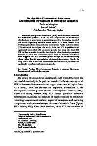
FIGURE 1(a). Partial correlation of private investment and volatility.

FIGURE 1(b). Partial correlation of public investment and volatility.

illustrates the partial correlation between the volatility index and private and public investment shares, respectively.7 The finding that volatility is negatively related to private investment and positively related to public investment can be rationalized in various ways. For example, if public investment is determined by a benevolent planner, it may increase in periods of heightened volatility to compensate for the reluctance of the private sector to invest. If public investment is a mechanism for distributing political rents in a rent-seeking society, then public investment may increase in periods of political instability. Thus, political instability triggers both the drop  The London School of Economics and Political Science 1999

1999]

VOLATILITY AND INVESTMENT

163

in private investment and the rise in public investment.8 Whatever the correct interpretation, the findings suggest that testing for a negative link between volatility and investment may be more successful when using disaggregated private investment data. Moreover, most theories examining the linkage between volatility and investment study the decisions of private agents. On balance, our results concerning the negative correlation between volatility and private investment are similar but stronger than those reported by Pindyck and Solimano (1993), who found that ‘the relationship [between volatility and investment] is negative but moderate in size and is of greater magnitude for developing countries’ (p. 297). Pindyck and Solimano cautioned that their results are subject to some important caveats since they worked with a sample of only 29 rich and poor countries and used several sources to obtain disaggregated investment data.9 Our larger sample, our exclusive focus on developing countries and our use of a common source for disaggregating total investment may help explain the stronger results we obtain. In addition, we focus on several volatility measures not used by Pindyck and Solimano, two of which (government spending shares and money growth) prove to be highly significant for both private and public investment.10 Ramey and Ramey (1995) use a panel of 92 rich and poor countries over the 1960–85 period in order to explore the relationship between volatility and growth. They find that their particular measure of volatility lowers growth but is not significantly related to investment. Since we have uncovered a strong negative correlation between our measures of volatility and private investment, we re-examine their claim using their methodology on our data of developing countries. We start by examining the relationship between growth and volatility where volatility is measured as the standard deviation of innovations to a forecasting equation for growth. For the analysis, we use the specification in Ramey and Ramey (1995): (1a)

∆yit Gλσ iCθ ′XitCε it ,

(1b)

ε it ∼ N(0, σ 2i ),

iG1, . . . , I; tG1, . . . , T,

where ∆yit is the growth rate of output per capita for country i in year t, expressed as a log difference; σ i is the standard deviation of the residuals, ε it ; Xit is a vector of control variables and forecasting variables; and θ is a vector of coefficients assumed to be common across countries. The residuals ε it are specified to be normally distributed and represent the deviation of growth from the value predicted based on the variables in X.11 The variance of the residuals, σ 2i , is assumed to differ across countries, but not across time. The standard deviation of the residuals is the volatility measure. The control variables included in X are the same as those used by Ramey and Ramey, who in turn select those judged important by Levine and Renelt. We use (1) initial log of real GDP per capita, (2) initial human capital as measured by secondary school enrollment, (3) the initial growth rate of the population, and (4) the average (public and private) investment fraction of GDP over the period.12 In addition, we follow Ramey and Ramey (1995) by including forecasting variables in our growth equation. These are (1) two lags of the log level of real  The London School of Economics and Political Science 1999

164

[MAY

ECONOMICA

GDP per capita, (2) a time trend and a time trend squared, (3) a time trend that starts in 1983 after the onset of the debt crisis, and (4) a dummy variable for 1983 and after. These forecasting variables permit various configurations for the estimated trend in GDP. Ramey and Ramey use similar forecasting variables, but they look for a possible break in the trend in 1974, after the first oil shock. Given that our data do not start until 1970, we look for a possible break in 1983, after the onset of the debt crisis. We estimate the model in (1) jointly using the same maximum likelihood procedure as in Ramey and Ramey. The time period begins in 1972 and runs through 1992, resulting in a panel of 966 observations for the 46 developing countries in the sample. As shown in Table 5(a), volatility enters the estimated growth equation with a negative coefficient that is statistically significant. Moreover, the negative relationship exists even though we control for the total investment share of GDP. Ramey and Ramey obtain the same results. We now check whether this particular volatility measure is significantly related to investment. Ramey and Ramey find that in the simple bivariate specification, innovation volatility appears to have a negative relationship with investment and is significant at the 10% level in their 92-country sample but is TABLE 5 RELATIONSHIP BETWEEN INVESTMENT AND INNOVATION VOLATILITY Specification (a)

Growth equation13 (coefficient on volatility)

(b)

Private investment equations (coefficient on volatility) Other variables included (besides a constant term) None Control variables

(c)

Total (public and private) investment equations (coefficient on volatility) None Control variables

(d)

Public investment equations (coefficient on volatility) None Control variables

46-country sample (996 observations) −0.2484 (−2.42)

−0.6371 (−2.50) −0.6866 (−2.26)

−0.2113 (−0.43) −0.3120 (−1.12) 0.3931 (0.89) 0.4024 (1.27)

Notes: The control variables are the initial log real GDP per capita, the initial secondary school enrollment rate, the initial population growth rate and the average trade share of GDP. Excluding the openness measure from the set of control variables to duplicate the control variables in Ramey and Ramey (1995) does not alter the results. Investment equations corrected for heteroscedasticity. Numbers in parentheses are t-statistics. Sources: Penn World Tables, Version 5.6a; Glen and Sumlinski (1995); Madarassy and Pfeffermann (1992); IMF International Financial Statistics; Inter-American Development Bank; Barro (1991) data.  The London School of Economics and Political Science 1999

1999]

VOLATILITY AND INVESTMENT

165

not significant in their 24-country OECD sample. However, once the control variables are included in the investment equation, the effect is no longer significant even in the bigger sample (Ramey and Ramey 1995, p. 1145). Table 5(b) shows the results of cross-country regressions of the average private investment share on innovation volatility for our set of 46 developing countries. In the simple bivariate specification, we find a negative relationship between innovation volatility and private investment spending that is statistically significant at the 5% level. The second row shows that the strong negative relationship between volatility and private investment continues to hold even after the control variables are included in the investment equation. Parts (c) and (d) of the table show that the correlation between innovation volatility and total investment is negative but not statistically significant, while the correlation between volatility and public investment is positive but insignificant. Thus, while Ramey and Ramey find little impact of innovation volatility on average total (public and private) investment shares, as do we, we uncover a negative and highly significant relationship between volatility and private investment, even after controlling for other factors. Our use of the private investment measure explains why our sample size is smaller and may also explain why our results are stronger.14 Since Ramey and Ramey find little evidence that the negative link between volatility and growth flows through the aggregate investment channel, they conclude that the adverse effects of volatility must work through other channels. For example, volatility may induce planning errors by firms or costly reallocation of resources across sectors. (See Ramey and Ramey 1991 and Dixit and Rob 1994 for further discussion.) We also find little evidence that the negative link between volatility and growth flows through the aggregate investment channel, but cannot rule out the possibility that in developing countries volatility also works through the private investment channel. We also constructed innovations by allowing for country-specific coefficients on the forecasting variables in equation (1a). Since computation is infeasible in the jointly estimated model because of the number of parameters, we followed the procedure in Ramey and Ramey (1995) of estimating separate growth forecasting equations for each country, containing a constant term, two lags of GDP and the four trend variables. We calculated the standard deviation of the innovation for each country from the estimated residuals of the country-specific growth equations. We then re-estimated equation (1a), which included the standard control variables and forecasting variables, by ordinary least squares using the full panel and obtaining heteroscedastic-consistent standard errors. The correlations between the standard deviation and the various investment measures are qualitatively the same as those reported in Table 5. The volatility measure is negatively and significantly correlated with private investment, but is uncorrelated with either total investment or public investment. We believe that the finding of a statistically significant negative partial correlation between a number of volatility measures and private investment in a set of developing countries lends support to the view that volatility has important detrimental effects on developing countries. It calls for a theory of behaviour under uncertainty that can deliver negative first-order effects of volatility on investment. We turn now to an exploration of some frameworks that deliver the observed first-order effects by relying on risk aversion or incomplete markets.  The London School of Economics and Political Science 1999

166

ECONOMICA

[MAY

II. GENERALIZED PREFERENCES AND UNCERTAINTY It is noteworthy that interest in generalized expected utility models goes beyond the interest in explaining the volatility–investment association. Savage’s (1954) expected utility maximization framework, while very useful in many contexts, has difficulties in explaining some ‘anomalies’ and modes of behaviour. For example, the excess volatility of stock prices reported by Shiller (1981) and the equity risk premium puzzle identified by Mehra and Prescott (1985) raise questions about the appropriateness of Savage’s approach. The Allais paradox (see Harless and Camerer 1994 for a review) suggests that there are interesting situations where the bias towards a known outcome impacts decision-making in ways that are not captured in Savage’s environment. These sorts of concern have led to the development of generalized expected utility approaches that relax Savage’s axioms. (See Epstein 1992 for a useful review of the new approaches to modelling risk.) While the debate about the merits of these new approaches is not yet settled, the new approaches deserve further theoretical and empirical investigation. We shall focus on two generalizations of Savage’s expected utility model: Gul’s (1991) disappointment aversion and Knightian uncertainty. They each offer a rationale for the large, negative association between volatility and investment, yet they do not rule out the potential importance of other factors like incomplete markets or lack of diversification. In fact, one suspects that in developing countries the interaction among all these factors plays an important role. The persistence of a large premium attached to equities (the ‘equity premium puzzle’) suggests, however, that risk aversion considerations cannot be dismissed by the mere existence of a ‘reasonably’ well functioning capital market. Disappointment aversion In the disappointment aversion model, agents maximizing expected utility attach more weight to ‘bad’ outcomes than to ‘good’ ones. Gul (1991) developed the framework in order to rationalize a seemingly paradoxical response of agents to two pairs of gambles. We present a simplified version of it to show that it delivers results consistent with our empirical findings. Since the model is a one-parameter extension of the standard neoclassical expected utility model, it allows one to assess the impact of volatility on investment when agents are disappointment-averse relative to the case where they are not. We start with a discussion of the Allais paradox, as this paradox and other anomalies shaped the development of Gul’s (1991) approach.15 Next, we review Gul’s formulation by considering the simplest case—a two-states-of-nature example. We use this example to highlight the general approach. Our purpose is to demonstrate that disappointment aversion provides one way to obtain first-order negative investment effects of volatility. No attempt is made to claim that the disappointment aversion framework is the only one that is consistent with the data. In fact, the work of Segal and Spivak (1990) suggests that similar effects may be produced by other versions of generalized expected utility. The Allais paradox arises out of a situation where agents confront two pairs of gambles. The first pair of gambles compares a safe bet to a lottery that involves a small probability of a large safe bet. In the second pair of  The London School of Economics and Political Science 1999

1999]

VOLATILITY AND INVESTMENT

167

gambles the agent confronts two lotteries that are rather similar in terms of the chance of disappointment. One offers marginally higher income in the ‘win’ state at a marginally lower probability relative to the second lottery. For certain parameter values, agents frequently prefer the safe bet in the first pair of gambles, and the lottery that offers the higher income at a marginally lower probability in the second pair. These choices are inconsistent with maximizing expected utility. Gul suggests that these choices may be consistent for agents who exhibit aversion to disappointment. If the benchmark for disappointment is the ‘certainty-equivalent’ income, agents may attach greater weight to circumstances where the realized income is below this benchmark. This leads to asymmetric weighting of states of nature and may explain the bias towards the safe bet exhibited in the Allais paradox. We turn now to a more formal description of Gul’s approach. The preferences of a disappointment-averse agent may be summarized by [u(x), β ], where u is a conventional utility function describing the utility of consuming x, [u′H0, u″F0], and β X0 is a parameter that measures the degree of disappointment aversion.16 Let V(β ) denote the expected utility of a disappointment-averse agent whose disappointment aversion rate is β . In the absence of risk, the agent’s utility level is simply u(x). Suppose there are two states of nature. With probability α the agent receives income x1 , and with probability (1Aα ), income x2 , where x1Hx2 . For this example, the disappointment-averse expected utility is defined by (2)

V(β )G[α u(x1 )C(1Aα )u(x2 )]Aβ (1Aα )[V(β )Au(x2 )],

where the first square-bracketed term on the right-hand side is the conventional expected utility in the absence of disappointment aversion and the second term is the degree of disappointment aversion (β ) multiplied by the expected disappointment.17 Rearranging terms in (2) yields (3)

V(β )G[α (1Aθ1 )]u(x1 )C[(1Aα )(1Cθ2 )]u(x2 )

where θ1 G(1Aα )κ H0, θ2 Gακ H0 and κ Gβ y[1C(1Aα )β ]H0. If the agent is disappointment-averse (β H0), he attaches an extra weight of (1Aα )θ2 to ‘bad’ states where he is disappointed (relative to the probability weight used in the conventional utility), and attaches a lesser weight of αθ1 to ‘good’ states (with (1Aα )θ2 Gαθ1 ). The parameter β measures the gap between the weights attached to the good and bad states of nature. Note that, for β G0, V is identical to the conventional expected utility. In this case, good and bad states of nature are treated symmetrically in weighting the utility measure. As we show below, weighting states of nature asymmetrically causes volatility to have firstorder effects, whereas symmetric weighting only leads to second-order effects. Figure 2 illustrates the welfare consequences of volatility when agents are disappointment-averse relative to the case where they are not. Consider the case where consumption, c, fluctuates between (1Aε) and (1Cε) and the probability of each state is 0.5. The bold curve (MU) traces the marginal utility of consumption for a risk-averse, disappointment-neutral agent (RH0, β G0), where R is the degree of risk aversion.18 We normalize units such that marginal utility at cG1 is 1. If β G0, volatility reduces expected utility approximately by the hatched triangle (>0.5ε [Rε]G0.5Rε2, drawn for εG0.05).  The London School of Economics and Political Science 1999

168

ECONOMICA

[MAY

FIGURE 2. Volatility and marginal utility. Figure 2 is drawn for the case where consumption fluctuates between (1Aε ) and (1Cε ), the probability of each state is 0.5, and ε G0.05. Curve MU is the marginal utility of consumption for RG2, β G0. Curve AB′BEE′D is the modified marginal utility of consumption for RG2, β G1.

If βH0, the relevant ‘marginal utility’ in the state of nature where cF1 and the agent is disappointed is MU{1C[0.5βy(1C0.5β )]}.19 The modified marginal utility is traced by curve AB′BEE′D and has a discontinuity at cG1. When the shock ε is zero, consumption is one and utility is u(1). In the good state, εG0.05 and the utility of a disappointment-averse agent exceeds u(1) by the trapezoid EE′HG. In the bad state, εG−0.05 and utility falls short of u(1) by the trapezoid B′BGF. Volatility reduces the expected utility of a disappointment-averse agent by half the difference between these two trapezoids. This loss in expected utility is depicted by the shaded trapezoid ( >[0.5βy (1C0.5β )] ε ). The loss is proportional to the degree of disappointment aversion since a higher β increases the size of the discontinuity. We now examine the role of disappointment aversion on the relationship between volatility and investment. We introduce a two-period example, where the only risk is a random investment return. To isolate the impact of firstorder risk aversion, we focus on the case where adjustment costs are zero.20 Utility is time-separable, and the agent exhibits disappointment aversion in the presence of risk. In period 1 the agent starts with an endowment of capital (K ) and some outside income (Z ). The first-period production function is f (K ), with f ′H0 and f ″F0. Period 2 income is random and is given by ZCf (KCI)(1Cλ), where λ is a random productivity shock, and I is the firstperiod investment. We assume two states of nature [λGε, − ε ], which occur with equal probability. The consumer chooses investment I so as to maximize a disappointmentaverse expected utility: (4)

V(β) u(ZCf (K )AI)C , 1Cρ

 The London School of Economics and Political Science 1999

1999]

VOLATILITY AND INVESTMENT

169

where ρ is the subjective discount factor, and V(β) is defined by (2). Applying (3) and (4), the agent maximizes (5)

u(ZCf (K )AI) C

0.5 1 {u[ZCf (KCI)(1Cε)]C(1Cβ)u[ZCf (KCI)(1Aε)]} 1Cρ 1C0.5β

and the resulting optimal investment is (6)

I>I0Cε

β 0.5

1 1C0.5β 2ΓCϑ (ε ), 2

where I0 is the rate of investment in the absence of volatility, ϑ (ε2 ) represents terms proportional to ε 2, and u′[ZCf (KCI)][1AR{f (KCI)y[ZCf (KCI)]}] , ΓG [u″( f (KCI))( f ′(KCI))2Cu′( f (KCI)) f ″ (KCI)]C(1Cρ)u″(ZCf (K )AI) where R is the coefficient of relative risk aversion, with RG−d(log u′(x))y d(log x).21 Thus, for small ε (6a)

β 0.5

dI>

1 1C0.5β 2 Γ dε

sign

3dε 4Gsign [Γ]G−sign 31ARZCf (KCI) 4 .

and (6b)

dI

f (KCI)

Several observations can be made about equation (6): 1. Volatility has first-order effects, proportional to the standard deviation of shocks, as long as the agent is disappointment averse.22 2. Increased volatility has a negative effect on investment as long as Zy[ f (KCI)]C1HR; as long as (one plus) the share of outside income relative to the risky income exceeds the coefficient of relative risk aversion.23 3. Even when utility u(c) has little concavity (as is the case for R≈0), volatility induces powerful negative effects on investment as long as the agent is disappointment averse. A higher coefficient of relative risk aversion and a lower share of outside income mitigate this effect. 4. If β G0, agents maximize a conventional expected utility. In this case, volatility has second-order effects on investment, proportional to the variance of shocks. 5. Aggregation across individuals may alleviate the adverse effects of volatility if shocks are idiosyncratic and a well-functioning domestic capital market enables the effective pooling of endowments. Thin financial markets in developing countries limit the availability of these pooling opportunities, however. Furthermore, the mitigating effects of pooling are not present when agents in developing countries face macroeconomic shocks and macroeconomic risk.24 6. The above model focuses on random productivity shocks as the source of volatility. Identical results about the impact of volatility can be obtained for other disturbances that lead to volatile profits, such as random tax rates  The London School of Economics and Political Science 1999

170

ECONOMICA

[MAY

or policies leading to volatile costs of variable inputs. For example, volatile inflation leads to volatile profits when there is incomplete indexation of the tax system, wages and product prices. Similarly, volatile fiscal policy that creates volatile domestic demand conditions leads to more volatile wages, prices and profits in the economy. The presence of quotas and non-traded goods magnifies the impact of fiscal volatility on costs and profits. The model discussed above provides one mechanism that links the volatility of profits to investment. Our empirical evidence is consistent with such a transmission mechanism if macroeconomic uncertainty leads to more volatile profits. Owing to data limitations, we do not attempt to identify the relevant channels through which macroeconomic uncertainty affects investment. Hence, our empirical analysis should not be viewed as testing or confirming any special transmission mechanism. To gain further insight about the impact of volatility on investment, we simulate the modified utility-maximizing model. We consider the case where (7)

f (K )GAK γ, [c]1AR u(c)G , 1AR

0FγF1, RX0,

and A and R are constants.

FIGURE 3. Volatility and investment. ρ G0.05, α G0.5, γ G0.7, RG0.5, KG1, AG7, ZG10.87.

Figure 3 traces the impact of volatility (measured by ε) on investment. The simulation’s calibration is done so that, in the absence of volatility, the optimal investment is 25% of initial GDP. Notice that in the conventional case (β G0) the demand for investment is almost independent of volatility for εF0.15; in contrast, volatility has first-order effects if βH0. Further insight about the cost of volatility may be obtained by calculating the agent’s willingness to pay for the elimination of volatility. For the case where εG0.2, we find in the simulation that the cost of volatility is practically  The London School of Economics and Political Science 1999

1999]

VOLATILITY AND INVESTMENT

171

zero if the consumer is disappointment-neutral, but it is 4.3% of GDP if the degree of disappointment aversion is β G1. Figure 3 reveals that, even when utility u(c) has little concavity (as is the case for RG0.5), uncertainty has first-order adverse effects on investment as long as the agent is disappointment-averse. The reason is that disappointment aversion causes the agent to treat ‘good’ and ‘bad’ states of nature asymmetrically, and this behaviour is independent of the concavity of the utility function. The asymmetric treatment of ‘good’ and ‘bad’ states of nature creates a nonlinearity. As a result, volatility creates first-order effects proportional to the product of the standard deviation and the degree of disappointment aversion, β. In contrast, the effect of uncertainty with conventional neoclassical utility typically hinges on the concavity of the utility function. Without kinks, the neoclassical utility framework produces only second-order effects of volatility that are proportional to the variance of shocks. Knightian uncertainty and investment In a recent contribution, Romer (1994) argues that any welfare assessment should take into account the costs of missing activities in the economy. Romer focuses on the case where commercial policy prevents some economic activities from taking place, but the logic of his argument should apply to activities that are missing because of uncertainty. If the creation of new activities is important for sustained growth, as has been suggested in the endogenous growth literature, then uncertainty that hinders the formation of new activities may ultimately reduce growth. New activities expose entrepreneurs to unknown conditions. Consequently, it may be impossible to specify the complete probability distribution for stochastic economic variables. Such a situation is referred to as Knightian uncertainty. It is different from risk, where there is a unique distribution that summarizes the stochastic environment. Models that formalize rational decision-making under Knightian uncertainty can be found in Schmeidler (1989) and Gilboa (1987), and applications can be found in Dow and Werlang (1992), Epstein and Wang (1994) and Aizenman (1997). The Schmeidler–Gilboa approach allows one to distinguish between risk aversion and Knightian uncertainty aversion. It shows that with Knightian uncertainty aversion agents adjust so as to avoid bearing uncertainty. Such a model may provide an explanation for the reluctance to embark on new activities—such as investment in manufacturing—in the presence of uncertainty.25

III. NONLINEAR BUDGET CONSTRAINTS AND UNCERTAINTY In neoclassical models, uncertainty does not have clear-cut effects. Technically, this result follows from the fact that, with linear intertemporal budget constraints, the restrictions imposed by conventional preferences and technology are not rich enough to sign the third-order moments. In practice, however, one may question the exclusive reliance on linear budget constraints in dealing with intertemporal problems. A large literature points out that incomplete information or enforcement problems often leads to credit rationing and introduces  The London School of Economics and Political Science 1999

172

ECONOMICA

[MAY

FIGURE 4. Investment in the face of a credit ceiling. (a) Saving, investment demand and the interest rate. (b) Variable investment demand. (c) Variable credit ceiling.

a nonlinearity into the budget constraint. We now illustrate how capitalmarket imperfections can lead to a negative relationship between uncertainty and investment. Suppose that the supply of credit facing a developing country is given by an inverted L-shape, as shown in Figure 4(a), where S0 is the credit ceiling. Suppose first that the credit ceiling is non-stochastic, and let Id be the demand for investment. Actual investment is given by IGMin {Id(r0 ), S0 }, where Id(r0 ) is the investment demand at rGr0 . Suppose now that the demand for investment fluctuates between a high-demand state, I dhGI0Cε, and a low-demand  The London School of Economics and Political Science 1999

1999]

173

VOLATILITY AND INVESTMENT

state, I dlGI0Aε, while the credit ceiling remains S0 . The realized investment is plotted in Figure 4(b). The credit ceiling hampers the expansion of investment in the high-demand state without moderating the drop in investment in the low-demand state. Thus, volatile investment demand reduces average investment in the presence of credit rationing. In the example, if the probability of each state of nature is one-half, volatility reduces the expected investment from I0 to I′GI0A0.5ε (see Figure 4(b)).26 There are several ways to introduce a credit ceiling. One way is to consider sovereign risk. If a country’s ability to borrow in international credit markets is restricted because of limits on enforceability, more volatile investment demand will reduce average investment as long as the credit ceiling does not perfectly adjust to accommodate investment demand. Moral hazard and adverse selection problems may also lead to credit rationing since the riskiness of individual borrowers and projects cannot be identified a priori (see Stiglitz and Weiss 1981).27 In these circumstances, it may be optimal to set the loan rate below the market-clearing value and to ration credit. In such models, uncertainty and incomplete information tend to reduce equilibrium investment. Volatility can also have large negative effects when credit ceilings are imposed on human-capital investments. In the absence of complete insurance markets, greater volatility tends to increase the dispersion of income among households and to reduce average investment in human capital as more households face credit ceilings (see Galor and Zeira 1993 and Aghion and Bolton 1991).28 IV. CONCLUSION Our study uncovers a statistically significant negative correlation between volatility and private investment in a set of over forty developing countries and provides several possible interpretations for this result. We show that nonlinearities created by generalized preferences or capital-market imperfections can generate first-order negative effects of volatility on investment, although there are surely additional channels at work. Moreover, the interactions among generalized preferences, capital-market imperfections and other factors may magnify the adverse effects of volatility identified in our study. These potential interactions are of concern in dealing with developing countries, where limited access to global capital markets may be the rule rather than the exception. Studying these interactions is an important task for future research. DATA APPENDIX TABLE A1

Country Egypt Ghana Ivory Coast Kenya Madagascar

Private Public investment investment share share (%) (%) 7.70 4.79 6.48 11.91 4.09

Fiscal surprise

Money surprise

Real exchange rate surprise

0.026 0.023 0.009 0.012 0.008

0.027 0.021 0.012 0.015 0.017

0.132 0.426 0.069 0.040 0.157

16.17 6.74 7.24 8.50 6.98

 The London School of Economics and Political Science 1999

174

[MAY

ECONOMICA

TABLE A1—continued

Country Malawi Mali Mauritius Morocco Nigeria Tanzania Tunisia Zimbabwe Costa Rica Dom. Republic El Salvador Guatemala Haiti Mexico Panama Argentina Bolivia Brazil Chile Colombia Ecuador Guyana Paraguay Peru Uruguay Venezuela Bangladesh India Indonesia Iran Korea Malaysia Nepal Pakistan Philippines Singapore Sri Lanka Thailand Turkey Fiji Papua New Guinea

Private Public investment investment share share (%) (%) 6.90 11.43 16.18 12.44 4.65 9.30 11.41 10.26 14.92 15.30 10.03 10.47 6.58 13.13 10.95 13.40 3.05 15.85 10.97 14.53 12.15 4.51 15.95 15.38 8.14 10.51 12.08 10.51 16.37 10.01 22.60 17.19 10.41 7.21 17.54 27.97 11.11 21.10 11.15 14.05 18.95

Fiscal surprise

Money surprise

Real exchange rate surprise

0.019 0.020 0.013 0.015 0.041 0.035 0.005 0.018 0.008 0.013 0.010 0.004 0.012 0.004 0.015 0.012 0.023 0.009 0.016 0.008 0.010 0.085 0.016 0.012 0.009 0.006 0.037 0.009 0.010 0.018 0.007 0.011 0.047 0.014 0.007 0.007 0.019 0.008 0.007 0.020 0.018

0.014 0.022 0.020 0.024 0.019 0.027 0.017 0.016 0.017 0.013 0.013 0.009 0.033 0.013 0.011 0.020 0.024 0.017 0.017 0.008 0.009 0.062 0.008 0.022 0.017 0.024 0.013 0.009 0.008 0.025 0.010 0.013 0.011 0.025 0.009 0.017 0.012 0.007 0.017 0.017 0.012

0.055 0.096 0.031 0.039 0.201 0.170 0.047 0.068 0.103 0.161 0.132 0.082 0.063 0.116 0.031 0.257 0.357 0.092 0.092 0.074 0.103 0.112 0.120 0.142 0.166 0.109 0.126 0.049 0.118 — 0.087 0.044 — 0.091 0.078 — 0.107 0.034 0.111 0.067 0.136

11.35 10.23 8.19 10.64 10.91 11.47 13.95 8.06 6.27 8.63 4.50 3.91 8.48 7.16 2.47 6.37 4.28 6.01 6.18 6.89 8.25 22.22 5.75 5.66 4.48 8.07 6.20 8.82 9.63 7.87 6.65 10.95 6.62 9.10 5.74 10.69 10.17 6.93 10.67 13.86 5.88

Table A1 lists the 46 developing countries in the data set, private and public investment shares of GDP in percentage terms from the World Bank, and volatility measures that are standard deviations of residuals from AR1 processes for fiscal, monetary and external variables. The data for the investment and growth regressions come primarily from the Summers–Heston Penn World Tables, Version 5.6a; private and public investment shares are from the World Bank data set; the human capital variable is from Barro (1991); and the money and real exchange rate variables used to construct volatility measures are from the IMF’s International Financial Statistics (IMF 1995) and the Inter-American Development Bank.

 The London School of Economics and Political Science 1999

1999]

VOLATILITY AND INVESTMENT

175

ACKNOWLEDGMENTS This paper is part of the NBER’s research programme in International Trade and Investment. It integrates and extends two NBER working papers (nos. 5386 and 5841). Any opinions expressed are those of the authors and not of the NBER. We thank Valerie Ramey for helpful information about the Ramey–Ramey (1995) study, and Lazar Dimitrov for research assistance. We are also grateful for helpful comments from two anonymous referees, Avinash Dixit, Gary Engelhardt, Henry Farber, Andrew Oswald, Adrian Pagan and Andrew Rose. Any errors are ours. NOTES 1. In principle, volatility and uncertainty are different phenomena. ‘Volatility’ refers to the tendency of a variable to fluctuate, while ‘uncertainty’ is present only when those fluctuations are unpredictable. In practice, volatile variables are frequently unpredictable. We use the two concepts interchangeably. 2. Caballero (1991, p. 286). For a comprehensive discussion and references, see Dixit and Pindyck (1994). 3. Earlier studies that uncover a negative correlation between volatility and economic performance include Aizenman and Marion (1993), who find negative effects of fiscal, monetary and inflation volatility measures on investment and growth rates; Hausmann (1994), who finds negative effects of terms-of-trade volatility; and Pindyck and Solimano (1993), who find a negative short-run effect of volatility in the marginal profitability of capital on investment spending. Ramey and Ramey (1995) uncover a strong negative relationship between real GDP volatility and the average growth rate of GDP. See Hausmann and Gavin (1995) for a comprehensive overview of the detrimental effects of volatility on investment and growth. 4. When some annual observations are missing, we construct averages using the remaining subsample. 5. While Dickey–Fuller tests fail to reject the hypothesis of a random walk in some cases, the power of the tests is limited. On a priori grounds, the variables cannot be random walks. If they are shares, they are bounded between zero and one, and if they are rates of change, they are bounded above and below by reasonable limits. We expect the policy variables to include a mean-reverting component. 6. The volatility variables are generated regressors. See Pagan (1984) for a discussion of the econometric issues related to generated regressors. If rational agents form their expectations about macroeconomic volatility according to the AR1 process specified, then there is no errors-in-variables problem and the standard errors of the coefficients attached to the volatility measures are consistent once they are corrected for heteroscedasticity. Obviously, one may debate whether agents do indeed use an AR1 process in forming expectations. In the end, we refrain from more complex constructions of volatility measures since we have a limited time series for each country’s macro variables. In order to evaluate the robustness of our findings to alternative specifications, we also examine the partial correlation between volatility and investment using the joint estimation procedure in Ramey and Ramey (1995). 7. There is one outlier (Guyana), but the partial correlations are robust to its exclusion. For example, without Guyana in the sample, the coefficient on the volatility index measure in the private investment regression is −2.81 with a t-statistic of −4.5036, while the relevant coefficient in the public investment regression is 2.08 with a t-statistic of 2.9351. 8. One way to discriminate between the two interpretations may be to evaluate the marginal productivity of private versus public investment. For example, one may estimate a Barro (1991) growth regression where the regressors are public and private investment shares, initial GDP, primary and secondary education, political uncertainty measures, a relative price distortion measure and the government consumption share of GDP. Estimating such a growth regression with developing country data, it can be shown that public capital does not make a significant contribution to growth whereas private capital does. While this is not a formal test of the merits of the two explanations, the result is consistent with a political economy interpretation. 9. They used the OECD to obtain public investment data for developed countries and the World Bank to obtain the same data for developing countries. Difficulties arise because the two data sources use different methods to account for public investment and because the OECD data is of poor quality, as noted by Barro and Sala-i-Martin (1995) in their work on related topics. 10. In Section III we show that capital market imperfections magnify the adverse effects of monetary and fiscal volatility on investment. 11. See the end of Table 5 for the estimates of the model specified in (1a)–(1b). 12. We also considered an alternative specification where the investment share in 1970, the initial year of the sample, is the fourth control so there is no future information in any of the control  The London School of Economics and Political Science 1999

176

ECONOMICA

[MAY

variables when jointly estimating (1a) and (1b). The correlations between the volatility measure and private, public and total investment were essentially identical in magnitude and significance to those reported below. 13. The growth equation estimation is reported below. It is based on a maximum likelihood procedure. When the initial total investment share replaces the average share as a control in the growth equation, the coefficients on volatility and their respective t-values are almost identical to those reported above. When the country-specific volatility measure is generated from separate growth forecasting equations for each country, the coefficients on volatility and their levels of significance are qualitatively the same as those reported above. The growth regression is: GrowthG0.0834A0.2484 (volatility)A0.0082 (initial per capita GDP) (3.24) (−2.42) (−0.97) C0.0234 (initial school enrollment rate)A0.3875 (initial population growth rate) (1.19) (−1.28) C0.1563 (average total investment share of GDP) (4.29) C0.2330 log (GDP−1)A0.2354 log (GDP−2 ) p(6.98) (−6.75) C0.0060 (trend)A0.0008 (trend-squared) (2.71) (−4.38) C0.0202 (post-1982 trend)A0.0028 (post-1982 dummy), (5.33) (−0.47) where the log likelihood is 1594.37, the Durbin–Watson statistic is 2.10, and numbers in parentheses are t-statistics. The Durbin–Watson statistic from the first stage of the two-stage arch regression is 1.99. While skewness–kurtosis tests of the residuals from the first and secondstage regressions statistically reject normality, the plots of the residuals displayed below suggest that the normality assumption is a fairly good approximation.

14. Ideally we would like to have enough data to determine how much of the difference in our results compared to those in Ramey and Ramey (1995) is due to the level of disaggregation in the investment measures, the mix of countries in the sample and the time period chosen. These data are not currently available, however. 15. For further discussion of how disappointment aversion explains patterns of individual behaviour in various controlled experiments, see Harless and Camerer (1994) and Epstein (1992). See Kandel and Stambaugh (1991) for an assessment of the limitations of Savage’s framework in accounting for the equity premium puzzle, and Epstein and Zin (1990) for an explanation of how ‘first-order’ risk aversion helps rationalize the observed equity premium. 16. Gul (1991) considers the more general case, where βX−1 and u may be either convex or concave. We focus on the case where βX0 because we restrict our attention to u″F0. 17. In the more general case, the agent faces risky income {xs } in n states of nature, sG1, . . . , n. Let µ denote the certain income that yields the same utility level as the risky income: V(b)G u( µ). In other words, let the consumer be indifferent between the prospect of a safe income µ and risky income {xs }. The agent reveals disappointment aversion if he attaches extra disutility to circumstances where the realized income is below µ. Expected utility can be expressed as

#

V( β ; {xs })G u(x)g(x) dxAβ

#

[u( µ)Au(x)]g(x) dx

µHx

GE(u(x))Aβ E[u( µ)Au(x)u µHx] Pr [ µHx] where g is the density function, E is the expectation operator, Pr [ µHx] is the probability that  The London School of Economics and Political Science 1999

1999]

VOLATILITY AND INVESTMENT

177

the certain income exceeds the risky income, and E(u( µ)Au(x)u µHx) is the expected value of the difference in utility under certainty and risk, conditional on the realized consumption being below the certainty equivalent consumption. The term E(u( µ)Au(x)u µHx) measures the average ‘disappointment’. The disappointment-averse expected utility equals the conventional expected utility, adjusted downwards by a measure of disappointment aversion ( β ) times the ‘expected disappointment’. 18. Figure 2 is drawn for εG0.05. The MU line is the marginal utility of consumption when RG 2, β G0. Curve AB′BEE′D is the ‘marginal utility’ of consumption for RG2, βG1. 19. This follows from the fact that (3) implies that 0.5(1Cβ ) 0.5 u(1Cε)C u(1Aε) VG 1C0.5β 1C0.5β 0.5(1Cβ ) 0.5 [u(1Cε)Au(1)]C [u(1Aε)Au(1)] Gu(1)C 1C0.5β 1C0.5β 0.5β 0.5β u′(1)εC 1C u′(1)(−ε) . >u(1)C0.5 1A 1C0.5β 1C0.5β

31

2

1

2

4

20. While in practice adjustment costs may play an important role in explaining investment decisions during the business cycle, Caballero (1991) shows that adjustment costs are of lesser importance in explaining why different approaches lead to conflicting results about the relationship between volatility and investment. 21. Equation (6) is the Taylor expansion of I around ε G0. 22. Note that the standard deviation of productivity shocks is ε. 23. This condition is likely to be satisfied for a reasonable range of parameter values. In a representative-agent economy, the outside income could be labour income, accounting for about twothirds of GDP. In a more disaggregated model, outside income would also include the part of capital income that is independent of the investment modelled in (6). Thus one plus the share of outside income relative to the risky income could be in the range of 3, easily exceeding a coefficient of relative risk aversion of 2 or less. The condition for increased volatility to have a negative effect on investment follows from the first-order condition. In the presence of disappointment aversion, a greater weight is given to the ‘bad’ states of nature. Under these circumstances the first-order effect of volatility on investment is determined by the impact of volatility on the expected marginal utility of investment in ‘bad’ states of nature, as is depicted by [∂2u(ZCf (KCI)(1Aε))]y∂ε ∂I (see the last term in (5)). It is straightforward to verify that sign

3

f (KCI) ∂2u(ZCf (KCI)(1Aε)) G−sign 1AR . ∂ε ∂I ZCf (KCI)

4

3

4

24. Although some of these macroeconomic shocks may, in principle, be pooled via the international capital markets, country-risk factors and the home bias exhibited by most portfolios suggest that agents in developing countries have limited ability to moderate the effects of shocks in this way. There is also a debate about the relevance of pooling opportunities for agents in developed economics. Shiller (1993), for example, argues that agents in developed countries have limited ability to pool and smooth shocks. 25. To illustrate the argument, suppose the only known characteristic regarding manufacturing is the range of the yields, and potential entrepreneurs have access to risk-free investment opportunities, yielding r0 . The manufacturing sector is composed of differentiated products such that each entrepreneur has the incentive to invest in a different variety. Investment in variety m requires capital Km . The return on investment in variety m is rm and is known to be bounded between rl and rh . In the absence of further information regarding the yield rm , one can proceed by constructing two statistics. The first is the ‘worse scenario’ wealth, denoted by W q . The second is the ‘expected wealth’ if one attaches a uniform prior to the distribution of yields in manufacturing, denoted by En(W). The shortcoming of En (W) is that it does not attach any weight to the uncertainty about the distribution of underlying yields in manufacturing. To correct this shortcoming, one can use a decision rule that maximizes a weighted average of the above two statistics UGφW q C(1Aφ )En (W), 0YφY1. As illustrated by Dow and Werlang (1992), the weight φ reflects the degree of ‘uncertainty aversion’ for a risk-neutral agent. In these circum˜ stances, investment in manufacturing is warranted only if rmAr0H(r0Arl )φy(1Aφ ), where ˜ rmG0.5[rhCrl ]. Hence, a uniform mean-preserving increase in the range of possible yields in manufacturing will make investment in manufacturing less likely. It will increase (r0Arl ) with˜ out affecting (rmAr0 ). Consequently, higher volatility will reduce investment in manufacturing.  The London School of Economics and Political Science 1999

178

ECONOMICA

[MAY

26. Figure 4 provides a minimal sketch of this argument. A more complete illustration of this point in an endogenous-growth, irreversible reinvestment model can be found in Aizenman and Marion (1993). See Fazzari et al. (1988) for an overview of financing constraints and corporate investment. 27. Gertler and Rogoff (1990) extend the Stiglitz–Weiss (1981) framework to the open economy. 28. If the demand for investment in human capital is similar across households (say, given by I d in Figure 4), the size of the initial wealth determines the effective credit ceiling facing the household. Let Ih,0 be the demand for investment in human capital at the risk-free interest rate. A household whose credit ceiling exceeds Ih,0 is unrestricted at the margin, investing Ih,0 . A household with low net worth finds the credit ceiling binding, investing less than Ih,0 . Thus investment in human capital depends on the credit ceiling facing a household, as plotted in Figure 4(c).

REFERENCES ABEL, A. (1983). Optimal investment under uncertainty. American Economic Review, 73, 228–33. AGHION, P. and BOLTON, P. (1991). A trickle-down theory of growth and development with debtoverhang. Working Paper, Delta, Paris. AIZENMAN, J. (1997). Investment in new activities and the welfare cost of uncertainty. Journal of Development Economics, 52, 259–77. —— and MARION, N. (1993). Policy uncertainty, persistence and growth. Review of International Economics, 2, 145–63. BARRO, R. (1991). Economic growth in a cross section of countries. Quarterly Journal of Economics, 106, 407–44. —— and SALA-I-MARTIN, X. (1995). Economic Growth. New York: McGraw-Hill. CABALLERO, R. J. (1991). On the sign of the investment–uncertainty relationship. American Economic Review, 81, 279–88. DIXIT, A. K. and PINDYCK, R. S. (1994). Investment under Uncertainty. Cambridge, Mass.: MIT Press. —— and ROB, R. (1994). Risk sharing, adjustment and trade. Journal of International Economics, 36, 263–87. DOW, J. and WERLANG, S. R. de Costa (1992). Uncertainty aversion, risk aversion, and the optimal choice of portfolio. Econometrica, 62, 197–204. EPSTEIN, L. G. (1992). Behavior under risk: recent developments in theory and applications. In L. Jean-Jacques (ed.), Advances in Economic Theory: Sixth World Congress, Vol. 1, Cambridge: Cambridge University Press, pp. 1–63. —— and WANG, T. (1994). Intertemporal asset pricing under Knightian uncertainty. Econometrica, 64, 283–322. —— and ZIN, S. E. (1990). ‘First-order’ risk aversion and the equity premium puzzle. Journal of Monetary Economics, 26, 387–407. FAZZARI, S. M., HUBBARD, R. G. and PETERSEN, B. C. (1988). Financing constraints and corporate investment. Brookings Papers on Economic Activity, 1, 141–95. GALOR, O. and ZEIRA, J. (1993). Income distribution and macroeconomics. Review of Economic Studies, 60, 35–52. GERTLER, M. and ROGOFF, K. (1990). North–South lending and endogenous capital-market inefficiencies. Journal of Monetary Economics, 26, 245–66. GILBOA, I. (1987). Expected utility theory with purely subjective non-additive probabilities. Journal of Mathematical Economics, 16, 65–88. GLEN, J. and SUMLINSKI, M. (1995). Trends in Private Investment in Developing Countries 1995. Discussion Paper no. 25, International Finance Corporation, World Bank. GUL, F. (1991). A theory of disappointment aversion. Econometrica, 59, 667–86. HARLESS, D. W. and CAMERER, C. (1994). The predictive utility of generalized expected utility. Econometrica, 62, 1251–90. HARTMAN, R. (1972). The effects of price and cost uncertainty on investment. Journal of Economic Theory, 5, 258–66. HAUSMANN, R. (1994). On the road to deeper integration with the North: lessons from Puerto Rico. Unpublished paper, Inter-America Development Bank. —— and GAVIN, M. (1995). Overcoming volatility. Special Report, Economic and Social Progress in Latin America. Washington, DC: Inter-America Development Bank. INTERNATIONAL MONETARY FUND (1995). International Financial Statistics (compact disk).  The London School of Economics and Political Science 1999

1999]

VOLATILITY AND INVESTMENT

179

KANDEL, S. and STAMBAUGH, R. F. (1991). Asset returns and intertemporal preferences. Journal of Monetary Economics, 27, 39–71. LEVINE, R. and RENELT, D. (1992). A sensitivity analysis of cross-country growth regressions. American Economic Review, 82, 942–63. MADARASSY, A. and PFEFFERMANN, G. (1992). Trends in Private Investment in Developing Countries, 1992 edn. International Finance Corporation Discussion Paper no. 14, World Bank. MEHRA, R. and PRESCOTT, E. (1985). The equity premium. Journal of Monetary Economics, 15, 145–61. NEWBERY, D. and STIGLITZ, J. (1981). The Theory of Commodity Price Stabilization. Oxford: Clarendon Press. PAGAN, A. (1984). Econometric issues in the analysis of regressions with generalized regressors. International Economic Review, 25, 221–48. PRATT, J. W. (1964). Risk aversion in the small and in the large. Econometrica, 32, 122–36. PINDYCK, R. (1988). Irreversible investment, capacity choice, and the value of the firm. American Economic Review, 78, 969–85. —— and SOLIMANO, A. (1993). Economic instability and aggregate investment. NBER Macroeconomics Annual, 8, 259–302. RAMEY, G. and RAMEY, V. A. (1991). Technology commitment and the cost of economic fluctuations. NBER Working Paper no. 3755, June. —— and —— (1995). Cross-country evidence on the link between volatility and growth. American Economic Review, 85, 1138–51. ROMER, P. (1994). New goods, old theory, and the welfare costs of trade restrictions. Journal of Development Economics, 41, 5–38. SAVAGE, L. J. (1954). Foundations of Statistics. New York: John Wiley. SCHMEIDLER, D. (1989). Subjective probability and expected utility without additivity. Econometrica, 57, 571–87. SEGAL, U. and SPIVAK, A. (1990). First-order versus second-order risk aversion. Journal of Economic Theory, 51, 111–25. SHILLER, R. (1981). Do stock prices move too much to be justified by subsequent changes in dividends? American Economic Review, 71, 421–36. —— (1993). Macro Markets: Creating Institutions for Managing Society’s Largest Economic Risks. Oxford: Oxford University Press. STIGLITZ, J. and WEISS, A. (1981). Credit rationing in markets with imperfect information. American Economic Review, 71, 393–410. SUMMERS, R. and HESTON, A. (1995). The Penn World Tables (Version 5.6a). WHITE, H. (1980). A heteroskedasticity-consistent covariance matrix estimator and a direct test for heteroskedasticity. Econometrica, 48, 817–38.

 The London School of Economics and Political Science 1999