Visual odometry and map fusion for GPS navigation assistance ´ Ignacio Parra and Miguel Angel Sotelo and David F. Llorca and C. Fern´andez and A. Llamazares Department of Computer Engineering University of Alcal´a 28882 Alcal´a de Henares, Spain Email:
[email protected]
Abstract—This paper describes a new approach for improving the estimation of the global position of a vehicle in complex urban environments by means of visual odometry and map fusion. The visual odometry system is based on the compensation of the heterodasticity in the 3D input data using a weighted nonlinear least squares based system. RANdom SAmple Consensus (RANSAC) based on Mahalanobis distance is used for outlier removal. The motion trajectory information is used to keep track of the vehicle position in a digital map during GPS outages. The final goal is the autonomous vehicle outdoor navigation in large-scale environments and the improvement of current vehicle navigation systems based only on standard GPS. This research is oriented to the development of traffic collective systems aiming vehicle-infrastructure cooperation to improve dynamic traffic management. We provide examples of estimated vehicle trajectories and map fusion using the proposed method and discuss the key issues for further improvement.
I. I NTRODUCTION Accurate global localization has become a key component in vehicle navigation, not only for developing useful driver assistance systems, but also for achieving autonomous driving. Autonomous vehicle guidance interest has increased in the recent years, thanks to events like the Defence Advanced Research Projects Agency (DARPA) Grand Challenge and lately the Urban Challenge. Recently, the development of traffic collective systems for vehicle-infrastructure cooperation to improve dynamic traffic management has become a hot topic in Intelligent Transportation Systems (ITS) research. Our final goal is the autonomous vehicle outdoor navigation in large-scale environments and the improvement of current vehicle navigation systems based only on standard GPS. The work proposed in this paper is particularly efficient in areas where GPS signal is not reliable or even not fully available (tunnels, urban areas with tall buildings, mountainous forested environments, etc). Our research objective is to develop a robust localization system based on a low-cost stereo camera system that assists a standard GPS sensor for vehicle navigation tasks. Then, our work is focused on stereo vision-based real-time localization as the main output of interest. The idea of estimating displacements from two 3D frames using stereo vision has been previously used in [1], [2] and [3]. A common factor of these works is the use of robust estimation
978-1-4244-9311-1/11/$26.00 ©2011 IEEE
832
N. Hern´andez and I. Garc´ıa Electronics Department University of Alcal´a 28882 Alcal´a de Henares, Spain
and outliers rejection using RANdom SAmple Consensus (RANSAC) [4]. In [2] a so-called firewall mechanism is implemented in order to reset the system to remove cumulative error. Both monocular and stereo-based versions of visual odometry were developed in [2], although the monocular version needs additional improvements to run in real time, and the stereo version is limited to a frame rate of 13 images per second. In [5] a stereo system composed of two wide Field of View cameras was installed on a mobile robot together with a GPS receiver and classical encoders. The system was tested in outdoor scenarios on different runs under 150 m. with a precision in the estimation of the travelled distance of 2-5%. In order to maintain consistency in long sequences of images, [6] and [7] introduce a local bundle adjustment. This local bundle adjustment tries to estimate the extrinsic parameter for the last 𝑛 cameras and the 3D points positions taking into account the 2D re-projections in the 𝑁 (with 𝑁 ≥ 𝑛) last frames. The solution is carried out taking advantage of the sparse nature of the Jacobian matrix of the error measure vector as described in [8]. Although these systems increase the final accuracy in the position estimation, their results are similar to those not using bundle adjustment (About 5% accuracy for [7] and errors in the order of meters for [6]). Reaching similar accuracy in monocular systems involves the use of very high resolution images as in [9] (2-3% with 5 768 × 1024 images) or a previously known 3D model of the environment to recover the real scale as in [10]. In our previous work [11] the ego-motion of the vehicle relative to the road is computed using a stereo-vision system mounted next to the rear view mirror of the car. Feature points are matched between pairs of frames and linked into 3D trajectories. Vehicle motion is estimated using the non-linear, photogrametric approach based on RANSAC. In this paper a solution based in a weighted non-linear least squares algorithm is tested in real environments with real traffic conditions. Results show a 20 times improvement in the medium distance to the ground truth data [12] and a better fit to the shape of the trajectory. The obtained motion trajectory information is then translated into a digital map to obtain global localization. The final goal is to perform the
localization of the vehicle during GPS outages. The rest of the paper is organized as follows: in section II the solution to the motion trajectory estimation is described; section III presents how the visual odometry trajectory information is converted and corrected with the digital map; in section IV the improvements achieved in the visual odometry system and the map fusion are shown on real data, and finally section V is devoted to conclusions and discussion on how to improve the current system performance in the future. II. V ISUAL O DOMETRY U SING W EIGHTED N ON - LINEAR ESTIMATION
The problem of estimating the trajectory followed by a moving vehicle can be defined as that of determining at frame 𝑖 the rotation matrix R𝑖−1,𝑖 and the translational vector T𝑖−1,𝑖 that characterize the relative vehicle movement between two consecutive frames (see Fig. 1).
linear method can lead to a non-realistic solution where the rotation matrix is not orthonormal. On the other hand, non-linear least squares is based on the assumption that the errors are uncorrelated with each other and with the independent variables and have equal variance. The Gauss-Markov theorem shows that, when this is so, this is a best linear unbiased estimator (BLUE). If, however, the measurements are uncorrelated but have different uncertainties, a modified approach might be adopted. Aitken showed that when a weighted sum of squared residuals is minimised, the estimation is BLUE if each weight is equal to the reciprocal of the variance of the measurement [13]. In our case, the uncertainty in the 3D position of a feature depends heavily on its location, making a weighted scheme more adequate to solve the system. This is due to the perspective model in the stereo reconstruction process. A Gaussianmultivariate model of the uncertainty is used to compensate for the heterodasticity in the input data. This solution based in a weighted non-linear least squares algorithm was developed, tested on synthetic data and compared to previous works in [12]. III. GPS ASSISTANCE USING O PEN S TREET M AP
Fig. 1.
Motion estimation problem
Given two triplets of 3D points at times 0 and 1 the equations describing the motion are: p1 = R0,1 ⋅ p0 + T0,1 ,
(1)
where p0 = [𝑥0 , 𝑦0 , 𝑧0 ]𝑡 and p1 = [𝑥1 , 𝑦1 , 𝑧1 ]𝑡 are the 3D coordinates of the points at times 0 and 1 respectively. Considering that there are only 6 unconstrained parameters (translational vector and 3 rotation angles) we need a minimum of 2 pairs of linked 3D points to get the solution. In practise, we will use as many points as possible to solve an overdetermined system. For this purpose a RANSAC based on non-linear leastsquares method was developed for a previous visual odometry system. A complete description of this method can be found in [11] and [12]. The use of non-linear methods becomes necessary since the 9 elements of the rotation matrix can not be considered individually (the rotation matrix has to be orthonormal). Indeed, there are only 3 unconstrained, independent parameters, i.e. the three rotation angles 𝜃𝑥 , 𝜃𝑦 and 𝜃𝑧 respectively. Using a
833
Map-matching algorithms use inputs generated from positioning technologies and supplement this with data from a high resolution spatial road network map to provide an enhanced positioning output. The general purpose of a map-matching algorithm is to identify the correct road segment on which the vehicle is travelling and to determine the vehicle location on that segment [14] [15]. Map-matching not only enables the physical location of the vehicle to be identified but also improves the positioning accuracy if good spatial road network data are available [16]. Our final goal is the autonomous vehicle outdoor navigation in large-scale environments and the improvement of current vehicle navigation systems based only on standard GPS. In areas where GPS signal is not reliable or even not fully available (tunnels, urban areas with tall buildings, mountainous forested environments, etc) this system will perform the localization during the GPS outages. Our research objective is to develop a robust localization system based on a low-cost stereo camera system that assists a standard GPS sensor for vehicle navigation tasks. To do so, the system controls the quality of the GPS signal based on the Horizontal Dilution Of Position (HDOP) from the GPS. When the signal is not reliable the last reliable position will be used as starting point and the motion trajectory computed from that point using the system explained before. Fusing the motion information provided by the visual odometry system with the topological information provided by OpenStreetMap (OSM) maps [17], we can keep track of our position until the GPS signal is recovered. In the next sections the nature of the topological information, the GPS signal quality assessment and the geolocalization using the motion trajectory data and the OSM maps are explained.
A. OpenStreetMap OpenStreetMap is a collaborative project to create a free editable map of the world. The maps are created using data from portable GPS devices, aerial photography, other free sources or simply from local knowledge. OSM data is published under an open content license, with the intention of promoting free use and re-distribution of the data (both commercial and non-commercial). OSM uses a topological data structure along with longitude and latitude information. It uses the WGS 84 latitude/longitude datum exclusively. The amount of information stored in the maps varies from one area to another but at least the following items can be found: ∙ Nodes: Points with a geographic position expressed in latitude and longitude. ∙ Ways: Lists of nodes, representing a polyline or polygon. They can represent buildings, parks, lakes, streets, highways, etc. ∙ Tags: can be applied to nodes, ways or relations and consist of name=value pairs. Examples of pieces of information stored in these tags are the king of way (highway, secondary, tertiary), orientation (oneway, twoways), name, speed limit, etc. In our system, the OSM maps can be downloaded at running time using OSM servers or can be downloaded offline and stored into a hard drive to be accessed on running time. Once the GPS signal is lost, the last reliable position is used to load an area of the OSM map surrounding that position. The map information is parsed and converted to Northing-Easting coordinates. All the conversions from and to WGS-84 latitude, longitude and ellipsoid height to and from Universal Space Rectangular XYZ coordinates has been performed using the equations in [18]. In this way, the motion information delivered by the visual odometry system in meters can be directly translated to the map and our new position is estimated. Finally our new position is converted back to longitude/latitude and sent to a server which will represent our trajectory in the map. B. Visual odometry and map fusion Traditionally GPS and Dead Reckoning (DR) has been used as input to map-matching algorithms however the conventional integration does not correct the position after re-location. Given the cumulative nature of errors in visual odometry estimations, the drift will keep increasing without bounding. Moreover, the complex nature of the urban environment and the numerous non-static objects (other cars, pedestrians,..) will make the map-matching process unreliable and eventually loose the vehicle position. If accurate localization is needed for long periods of GPS outage additional information available in the digital map has to be used to correct the actual vehicle position and reset the cumulative errors from visual odometry. Otherwise, small misestimations due to poor quality of the input images (rain, glares,...) or non-static objects, can quickly lead to mislocalizations. In our approach, we propose a probabilistic map-matching algorithm constrained to the road which uses map features
834
to control the errors of the visual odometry by feeding back corrections from the map-matching process. Every time the map-matching algorithm correctly matches the vehicle position at one of these features the vehicle position and heading is corrected. This calibration process (see Figure 2) looks for sharp turns and roundabouts and correct the vehicle position removing the cumulative error of the visual odometry. This idea is based on the previous work in [19] where GPS and DR were fused using a similar approach. The motion trajectory information is filtered and downsampled to 1 position per second to emulate the sampling rate of the real GPS. This way the user will not notice the difference between the GPS or the visual odometry fix. The actual position of the vehicle is represented as a distance from a map node and an orientation with respect to the segment between the two nodes the car is on. The car position is forced to be in the segment between nodes, what is usually known as lock on road on commercial GPS’s. As long as the vehicle moves, its position in the map is updated according to the input from the visual odometry system. 1) Integration of Visual Odometry and GPS: The signal from each GPS satellite has level of precision; depending on the relative geometry of the satellites. When visible GPS satellites are close together in the sky, the geometry is said to be weak and the Dilution Of Position (DOP) value is high; when far apart, the geometry is strong and the DOP value is low. In our system when the HDOP is greater than 10 the signal is considered to be not reliable and the position in the map is computed using the visual odometry information (see Figure 2).
Fig. 2.
Integration of the GPS and VO measures
2) Identification of the actual link: The most complex element of any map-matching algorithm is to identify the actual link among the candidate links [14]. In our mapmatching algorithm 3 basic assumptions are made: 1) The vehicle travels on the road most of the time. 2) The vehicle can not jump from one place to another one with no connection. 3) The vehicle has to follow certain road rules. Firstly the initial road segment in which the vehicle is travelling is estimated through an initialization process; when the GPS fix is lost an elliptical confidence region is computed using the visual odometry uncertainty and the last reliable GPS fix. The confidence region is projected into the map and
the road segments that are within the confidence region are taken as candidate regions (see Figure 3 ). For simplicity the elliptical confidence region is approximated to a rectangular one.
Fig. 3. Elliptical confidence region (red) and candidate segments blue) over the converted OSM map of Alcal´a de Henares
If the confidence region contains more than one candidate segment, the heading over the last 5 seconds is computed and compared to the segments orientation. If there is only one candidate left after the heading check, that is the initial road segment. If not, the distance from the motion trajectory to the segment is computed as follows: 1) Compute the starting point using the point-to-curve algorithm [20] for the last GPS fix. 2) Compare the estimated run distance to the distance left on the starting point segment. If it is greater than the distance left discard the starting point segment and go to step 3. Otherwise the starting point segment is the initial segment. 3) Compute the distance from the motion trajectory estimation to the candidate segments by computing the area under the motion estimation trajectory to a stretch of each one of the candidate segments. This stretch will have the same length as the motion trajectory estimation for all the candidate segments (see Figure 4) [20]. 4) Select the segment closer to the curve as the initial segment.
3) Tracking of the vehicle position in the map: After setting the initial position of the vehicle in the map subsequent motion estimations from the visual odometry are matched in the map following a different approach. Firstly the vehicle velocity, heading and position uncertainty are used to estimate if the vehicle is turning or driving trough a junction. If so, the identification of the actual link is started. Otherwise a simple tracking of the vehicle position in the map is performed (see Figure 5). The steps of this process are: 1) If the difference between the heading of the vehicle and the current road segment is higher than a threshold or there is at least one juncture in the uncertainty region start the identification of the actual link. If this process was triggered by the heading but not by the uncertainty region increase the uncertainty region a 20%. If not continue. 2) Using the vehicle heading and velocity, check the predicted position and the measured one, if close feedback the position to the visual odometry. The position in the road is computed using the point-to-curve algorithm and the heading is the road segment orientation.
Fig. 5.
Map-matching flow diagram.
This localization process is repeated until the GPS HDOP is greater than 10, then the GPS position fix will be used again. IV. I MPLEMENTATION AND R ESULTS
Fig. 4.
The system described in this paper was implemented in a QuadCore Q9550 at 2.83GHz with a GNU/Linux 2.6.27-16server kernel version. The algorithm was programmed in C using OpenCV libraries. A stereo vision platform based on Basler scA640 74-fm cameras was installed in the prototype vehicle. The stereo sequences were recorded using an external trigger signal for synchronization at 30 fps with a resolution of 640x480 pixels in grayscale. All sequences correspond to real traffic conditions in urban environments with non stationary vehicles and pedestrians. The test vehicle was part of a Floating Car Data (FCD) which collected information about the current traffic state. Each vehicle, which can be seen
Implemented curve-to-curve map-matching algorithm.
835
as a moving sensor that operates in a distributed network, is equipped with global positioning and communication systems, transmitting its global location, speed and direction to a central control unit that integrates the information provided by the vehicles. The results of the visual odometry system alone are summarized in table I along with ground truth data from GPS and Real Time Kinematic RTK-GPS. The accuracy in the trajectory estimation is very high specially taking into account that they were recorded in real traffic conditions with many non stationary cars crossing the scene and strong glarings and shadows. Also an example of the performance of the system in a tunnel is provided.
truth for a loop closure of 1.1Km are shown. In this case the input video images are of poor quality as a result of glares on the windscreen and dazzling of the cameras. Several cars and one pedestrian crossed with the test vehicle while driving. Still, the system was able to correctly reconstruct the trajectory with a very high accuracy using only visual information and no prior knowledge of the environment. On Fig. 7 the VO results for a 680m experiment in tunnel are shown. In this case the accuracy is lower (3%) due to strong shadows and glarings at the tunnel’s entrance and exit.
Visual Odometry 2D Trajectory Estimation Video 00 May 8th VO GPS RTK GPS
0
−50
z (m)
−100
−150
Fig. 8. Vehicle motion trajectory in the OSM and GPS information as shown to the user for the tunnel experiment.
−200
−250
−100
−50
0
50
100
150
200
250
x (m)
Fig. 6. Reconstructed trajectory for a 1.1km loop using visual odometry alone (solid line). GPS used as ground truth (circles) and RTK-GPS used as ground truth (diamons).
Estimated Trajectory for Video 05 May 8th RTK GPS GPS VO 250
200
z (m)
150
100
Fig. 9. Vehicle motion trajectory in the OSM and GPS information as shown to the user for the urban canyon experiment.
50
0 −300
−250
−200
−150
−100
−50
0
x (m)
Fig. 7. Reconstructed trajectory for a 680m trajectory using visual odometry alone (solid line). GPS used as ground truth (circles) and RTK-GPS used as ground truth (diamons).
On Fig. 6 the VO results, the RTK-GPS and GPS ground
836
In Figures 8 and 9 the output as shown to the user is shown for the tunnel and the urban canyon experiments. The mapmatching algorithm output (latitude and longitude positions) are fed to the Java interface to OSM, Travelling Salesman [21], which performs the map rendering and trajectory representation. As shown in Figure 8 the vehicle runs through a roundabout and a tunnel. The global position of the vehicle is tracked with no mistakes and the errors of the visual
TABLE I G ROUND TRUTH AND ESTIMATED LENGTHS USING VO ALONE FOR EXPERIMENTS
Loop closure Urban Canyon Tunnel
dGPS (m) Lost Lost 679
GPS (m) 1098.1 418.2 643.96
VO (m) 1101.5 421.14 700.63
Distance Error (%) 0.31 0.41 3.19
odometry are corrected by the map matching algorithm. The map-matching algorithm correctly estimates all the turnings and the exit for the roundabout. Other cars and buses present on the video sequence do not affect the global localization accuracy. V. CONCLUSIONS AND FUTURE WORKS A. Conclusions We have described a new method for estimating the vehicle global position in a network of roads by means of visual odometry. To do so, a new weighted non-linear scheme, to represent the input data nature, has been explained and tested. To improve the outlier removal Mahalanobis distance and RANSAC has been used. The resulting motion information has been used to get the global position of the vehicle in OSM. Both systems have been used to compensate the GPS outages, performing the global localization of the vehicle when the GPS signal is not available. The system has been implemented and tested on real traffic conditions. We provide examples of estimated vehicle trajectories as well as of the estimation of the global position in a map. Results show that the system is capable of compensating the GPS outages and provide the global position to the user. The cumulative error from the visual odometry system is compensated using the topological information of the map. This indicates that longer outages can be corrected. B. Future Works As part of our future work we envision to develop a method for discriminating stationary points for those which are moving in the scene. Moving points can correspond to pedestrians or other vehicles. The ego-motion estimation will mainly rely on stationary points. The system can benefit from other vision-based applications currently under development and refinement in our lab, such as pedestrian detection and ACC (based on vehicle detection). The output of these systems can guide the search for stationary points in the 3D scene. Also longer runs of several kilometers have to be performed to estimate the correcting capability of the map fusion. ACKNOWLEDGMENT This work has been supported by the Spanish Ministry of Innovation and Science by means of GUIADE (P9/08) and TRANSITO (TRA2008-06602-C03-03) projects.
837
Loop Error (m) 2.48 -
Loop Error (%) 0.2 -
R EFERENCES [1] Z. Zhang and O. Faugueras, “Estimation of displacements from two 3-d frames obtained from stereo,” IEEE Transactions on Pattern Analysis and Machine Intelligence, vol. 14(12), pp. 1141–1156, December 1992. [2] D. Nister, O. Narodistsky, and J. Beren, “Visual odometry,” Proceedings of the IEEE Conference on Computer Vision and Pattern Recognition, June 2004. [3] A. Hagnelius, “Visual odometry,” Master’s thesis, Umea University, Umea, 2005. [4] D. A. Forsyth and J. Ponce, Computer Vision. A modern Approach. Pearson Education International: Prentice Hall, 2003. [5] M. Agrawal and K. Konolige, “Real-time localization in outdoor environments using stereo vision and inexpensive gps,” 18th International Conference on Patter Recognition (ICPR06), pp. 1063–1068, 2006. [6] E. Mouragnon, M. Lhuillier, M. Dhome, F. Dekeyser, and P. Sayd, “Real time localization and 3d reconstruction,” Proceedings of the Conference on Computer Vision and Pattern Recognition (CVPR), pp. 363–370, 2006. [7] K. Konolige, M. Agrawal, and J. Sol´a, “Large scale visual odometry for rough terrain,” Proceedings of the International Symposium on Research in Robotics (ISRR), 2007. [8] R. Hartley and A. Zisserman, Multiple View Geometry in Computer Vision. Cambridge University Press, 2004. [9] J.-P. Tardif, Y. Pavlidis, and K. Danilidis, “Monocular visual odometry in urban environments using an omnidirectional camera,” Intelligent Robots and Systems (IROS), pp. 2531–2538, October 2008. [10] P. Lothe, S. Bourgeois, F. Dekeyser, E. Royer, and M. Dhome, “Towards geographical referencing of monocular slam reconstruction using 3d city models: Application to real-time accurate vision-based localization,” Conference on Computer Vision and Pattern Recognition (CVPR), pp. 2882–2889, 2009. [11] I. Parra, M. Sotelo, D. F. Llorca, and M. O. na, “Robust visual odometry for vehicle localization in urban environments,” ROBOTICA, vol. 28, pp. 441–452, May 2010. [12] I. Parra, M. Sotelo, D. F. Llorca, and C. Fern´andez, “Visual odometry for accurate vehicle localization - an assistant for gps based navigation,” 17th International Intelligent Transportation Systems World Congress, pp. 1–6, October 2010. [13] A. C. Aitken, “On least squares and linear combinations of observations,” Proceedings of the Royal Society of Edinburgh, vol. 55, pp. 42– 48, 1935. [14] J. S. Greenfeld, “Matching gps observations to locations on a digital map,” Proceedings of the 81st Annual Meeting of the Transportation Research Board, January 2002. [15] M. A. Quddus, W. Y. Ochieng, and R. B. Noland, “Current mapmatching algorithms for transport applications: State-of-the-art and future research directions,” Transportation Research Part C, vol. 15, pp. 312–328, 2007. [16] W. Ochieng, M. Quddus, and R. Noland, “Map-matching in complex urban road networks,” Brazilian Journal of Cartography, vol. 55, pp. 1–18, 2004. [17] “Openstreetmaps,” 2010. [Online]. Available: http://wiki.openstreetmap.org [18] L. S. H. and S. T. A., Electronic Surveying and Navigation. John Wiley & Sons, 1976. [19] C. Wu, Y. meng, L. Zhi-lin, C. Yong-qi, and J. Chao, “Tight integration of digital map and in-vehicle positioning unit for car navigation in urban areas,” Wuhan University of Natural Sciences, vol. 8, pp. 551–556, 2003. [20] A. K. D. Bernstein, “An introduction to map matching for personal navigation assistants,” 2002. [21] “Travelling salesman,” 2010. [Online]. Available: http://wiki.openstreetmap.org/wiki/Travelling salesman