arXiv:astro-ph/0106098v1 6 Jun 2001

THE XMM–NEWTON Ω PROJECT J.G. BARTLETT1,2 , N. AGHANIM3 , M. ARNAUD4 , J.–PH. BERNARD3 , A. BLANCHARD1 , M. BOER5 , D.J. BURKE6 , C.A. COLLINS7 , M. GIARD5 , D.H. LUMB8 , S. MAJEROWICZ4 , PH. MARTY3 , D. NEUMANN4 , J. NEVALAINEN8 , R.C. NICHOL9 , C. PICHON10 , A.K. ROMER9 , R. SADAT1 , C. ADAMI (associate) 1. Observatoire Midi–Pyr´en´ees, Toulouse, France 2. CDS, Strasbourg, France 3. Institut d’Astrophysique Spatiale, Orsay, France 4. SAp, CEA, Saclay, France 5. CESR, Toulouse, France 6. CfA, Cambridge, USA 7. Liverpool John Moores University, UK 8. Astrophysics Division, ESA/ESTEC 9. Carnegie Mellon University, Pittsburgh, USA 10. Observatoire de Strasbourg, Strasbourg, France The abundance of high–redshift galaxy clusters depends sensitively on the matter density ΩM and, to a lesser extent, on the cosmological constant Λ. Measurements of this abundance therefore constrain these fundamental cosmological parameters, and in a manner independent and complementary to other methods, such as observations of the cosmic microwave background and distance measurements. Cluster abundance is best measured by the X–ray temperature function, as opposed to luminosity, because temperature and mass are tightly correlated, as demonstrated by numerical simulations. Taking advantage of the sensitivity of XMM–Newton, our Guaranteed Time program aims at measuring the temperature of the highest redshift (z > 0.4) SHARC clusters, with the ultimate goal of constraining both ΩM and Λ.

1

Cluster abundance and Cosmology

In standard models, structures form from the collapse of density perturbations described by a Gaussian random field (in the linear regime). An object collapses once the density contrast δ ≡ (ρ − ρ¯)/¯ ρ (where ρ is the density field) reaches a critical value ∼ 1. The abundance of such regions will reflect the Gaussian nature of the perturbations, as will the mass function giving the number density of objects as a function of mass M and redshift z. Using simple statistical arguments of this kind, Press & Schechter 21 (PS) suggested the following formula for the mass function dn d ln M

=

r

d ln σ −ν 2 /2 2 ρ¯ e ν(M, z) πM d ln M



(1)

ν(M, z) ≡ δc /σ(M, z)

where δc is a (weakly) cosmology–dependent threshold (∼ 1.68) and σ(M, z) is the density perturbation amplitude at scale M . We see the underlying statistical nature of the perturbations

in the Gaussian cut–off at the high–mass end. Expressions for the mass function found in large numerical simulations differ somewhat from the PS form, but are well described by similarly simple analytic expressions 15 . Clusters reside on the high–mass tail (where σ < 1) and their abundance at any z is therefore highly sensitive to σ(M, z) = σ(M, z = 0)Dg (z; ΩM , Λ)

(2)

Here Dg is the growth factor for linear perturbations, which depends on the cosmology (ΩM , Λ). Perturbations freeze–out, i.e., slow their growth rate, in low–density models when the expansion becomes dominated by either the curvature term or a cosmological constant; Dg thus depends primarily on ΩM , and to a lesser extent on Λ. The presence of a cosmology–dependent factor in the exponential of the mass function implies that cluster abundance is an effective way to constrain these cosmological parameters. Constraints obtained in this manner are complementary to, for example, those found by observations of supernovae type Ia or by measurements of cosmic microwave background anisotropies that essentially rely on a determination of cosmological distance (luminosity or angular–size distances). 2

X–ray Temperature

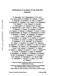
Strictly speaking, one requires the abundance of clusters as a function of their mass, a difficult quantity to measure directly. In practice, one seeks a direct observable that is closely related to virial mass. Lensing surveys would seem the most suited to the task, as the effects of lensing are of course directly related to mass (although projected along the line–of–sight). Among X– ray observables, temperature is a much more robust quantity than the luminosity, the latter depending on the density profile of the intracluster gas whose physics is currently difficult to model. The X–ray temperature, on the other hand, is expected to be tightly correlated with virial mass, an expectation borne out by numerical simulations 11,6 . Cluster abundance, and its evolution, is thus well measured by the X–ray temperature function dn/dT (T, z). With a calibrated T − M relation, the mass function is easily translated into a temperature function that may be compared with observations. The exact T − M relation to use is of course a critical issue, one that may be addressed, for example, using numerical simulations, or directly from detailed observations that determine both cluster mass and temperature, e.g., 17 . Figure 1 compares the predictions for a critical and an open model, both normalized to the present–day, observed dn/dT . Evolution towards higher redshift is strikingly different in the two models, illustrating the power of measurements of cluster abundance at z > 0 as a cosmological probe19 . This probe has been applied by numerous authors, yielding a variety of results on ΩM 20,13,2,3,24,5,10,16,22,25 . Use of the cluster abundance as a cosmological probe requires a well–controled sample with temperature measurements. There are several estimates of the local temperature function at z = 014,9,4 . For many years, the EMSS 12 played the central role for studies at z > 0; Henry 13 used this sample to find the temperature function at z ∼ 0.3, which is still the most distant temperature function determinated to date. In addition, there are now several X–ray selected catalogs based on serendipitous cluster detections in ROSAT pointings that are being used for cluster evolution studies. Efforts are underway to obtain temperatures for these samples using the new X–rays satellites, Chandra and XMM–Newton, but as yet there are no conclusive results. Temperature measurements are difficult to obtain because they require many photons to construct an X–ray spectrum; this is of course the reason the temperature function is still only poorly known at z > 0. Another avenue to the cluster abundance at high redshift is to apply a luminosity–temperature relation to a flux–limited sample, thereby obtaining either the temperature function, or a redshift distribution at given temperature. The advantage is that the

Figure 1: The predicted X–ray temperature function at redshifts z = 0 (solid), 0.3 (dashed) and 0.5 (dot–dashed) for a critical (blue) and an open (red) model (Λ = 0), both fitted to the local (z = 0) temperature abundance.

luminosity–temperature relation may be determined over a range of redshifts with few objects, and then applied to the much larger parent catalog 24 . In either case, whether one wishes to directly determine the temperature function, or use a constrained luminosity–temperature relation on a large flux–limited sample, temperature measurements for a number of clusters at high redshift are needed. This is the goal of our XMM– Newton Ω–project based on the SHARC cluster sample.

3

The SHARC Sample

The Serendipitous High–redshift Archival ROSAT Cluster (SHARC) survey consists of sources found to be extended by a wavelet analysis in ROSAT pointings. The catalog consists of objects found in two separate surveys: the Deep SHARC 7,8 , covering 17 square degrees in the South to a flux limit of fx [0.5 − 2keV] > 4 × 10−14 ergs/s/cm2 ; and the Bright SHARC 18,23 , covering 178 square degrees to fx [0.5 − 2keV] > 1.5 × 10−13 ergs/s/cm2 . This two–fold strategy yields a cluster catalog that straddles L∗ over 0.2 < z < 0.8 (see Figure 2). The selection function for the SHARC has been extensively studied 1 . 4

The XMM–Newton Project

As mentioned, the difficulty in obtaining temperatures for high–redshift clusters lies in collecting enough photons. The large collecting area of XMM–Newton makes it an ideal instrument for the task. Our Guaranteed Time (GT) program aims to establish the luminosity–temperature relation and to estimate the temperature function at the highest possible redshifts. To this end,

Figure 2: The SHARC luminosity function.

we will observe 7 of the most distant SHARC clusters, all at z > 0.4 (median of z = 0.5), to find their temperatures to ∼ 10% accuracy. Our consortium consists of GT holders from the EPIC, SOC and SSC XMM teams, and the SHARC team. The total observing time on the GT program amounts to 260 ksecs for the 7 objects, plus an additional cluster from another GT program obtained by mutual agreement; the program will continue on Guest Observing (GO) time with 160 ksecs already allocated after the first AO. With the 7-8 temperature measurements on the GT program, we will directly construct the temperature function at the highest redshifts yet reached. As the ability to distinguish models improves rapidly with redshift, due to the fact that clusters lie ever farther out on the Gaussian tail at early times, we hope to significantly improve constraints on ΩM and Λ from this key cosmological probe. In addition, the results will be based on a cluster catalog entirely independent of the workhorse EMSS, and therefore with different possible systematics, which will help to control possible hidden systematics in the method. Acknowledgments Our thanks to the organizers for an enjoyable and exciting meeting, and to the local staff for their constant attention and care. References 1. 2. 3. 4.

C. N. A. A.

Adami, M.P. Ulmer, A.K. Romer et al., Ap.J.S. 131, 391 (2000) Bahcall & X. Fan, Ap.J. 504, 1 (1998) Blanchard & J.G. Bartlett, A&A 314, 13 (1998) Blanchard, R. Sadat, J.G. Bartlett & M. Le Dour, A&A 362, 809 (2000)

5. 6. 7. 8. 9. 10. 11. 12. 13. 14. 15. 16. 17. 18. 19. 20. 21. 22. 23. 24. 25.

S. Borgani, P. Rosati, P. Tozzi & C. Norman, Ap.J. 517, 40 (1999) G.L. Bryan & M.L. Norman, Ap.J. 495, 80 (1998) D.J. Burke, C.A. Collins, R.M. Sharples et al., Ap.J. 488, L83 (1997) C.A. Collins, D.J. Burke, A.K. Romer et al., Ap.J. 479, L117 (1997) A.C. Edge, G.C. Stewart, A.C. Fabian & K.A. Arnaud, MNRAS 245, 559 (1990) V.R. Eke, S. Cole, C.S. Frenk & J.P. Henry, MNRAS 298, 1145 (1998) A.E. Evrard, C.A. Metzler & J.F. Navarro, Ap.J. 469, 494 (1996) I.M. Gioia, T. Maccacaro, R.E. Schild, Ap.J.S. 72, 567 (1990) J.P. Henry, Ap.J. 489, L1 (1997) J.P. Henry & K.A. Arnaud, Ap.J. 372, 410 (1991) A. Jenkins, C.S. Frenk, S.D.M. White et al., MNRAS 321, 372 (2001) M. Markevitch, Ap.J. 504, 27 (1998) J. Nevalainen, M. Markevitch & W. Forman, Ap.J. 532, 694 (2000) R.C. Nichol, A.K. Romer, B.P. Holden et al., Ap.J. 521, L21 (1999) J. Oukbir & A. Blanchard, A&A 262, 21 (1992) J. Oukbir & A. Blanchard, A&A 317, 1 (1997) W.H. Press & P. Schechter, Ap.J. 187, 425 (1974) D.E. Reichart, D.Q. Lamb, M.R. Metzger et al., Ap.J. 518, 521 (1999) A.K. Romer, R.C. Nichol, B.P. Holden et al., Ap.J.S. 126, 209 (2000) R. Sadat, A. Blanchard & J. Oukbir, A&A 329, 21 (1998) P.T.R. Viana & A.R. Liddle, MNRAS 303, 535 (1999)