Using the randomization in specifying the ANOVA model and table for grazing trials By C.J. BrienA and C.G.B. DemétrioB A

School of Mathematics, University of South Australia, North Terrace, Adelaide, SA 5000, Australia. Email: [email protected] B Departamento de Matemática e Estatística, ESALQ, Universidade de São Paulo, Caixa Postal 9, 13418-900 Piracicaba, SP, Brasil. Short title: Specifying the ANOVA model and table for grazing trials Summary. A method for deriving the analysis of variance for an experiment is presented and applied to grazing trials. A special feature of grazing trials, specifically utilized by our method, is that they involve at least two randomizations: treatments are randomized to field units (for example paddocks or plots) and field units are randomized to animals. Randomization results in the confounding (‘mixing up’) of terms and our method includes separate terms in the analysis of variance table for confounded terms so that all sources of variability in the experiment have terms for them included in the table and the confounding between the sources of variability in the experiment is explicitly displayed in the table. This information is employed in determining the valid error terms and we will present examples that show how to ascertain these for effects of interest and hence which effects can be tested. In this it fulfils the same role as the contentious process of identifying the experimental unit. It will be demonstrated that the inclusion of separate terms for confounded terms results in improper replication in grazing trials being automatically signalled, and makes its ramifications clear. Keywords. analysis of variance; confounding; error terms; experimental unit; fixed factors; multitiered experiments; replication; random factors; randomization; tiers Introduction A design for a grazing trial must provide valid error terms and sufficient precision for the effects of interest — that is, there must be proper and adequate replication. As Drane (1989, p.78) states `the manner in which the experiment is designed and executed determines what constitutes the experimental unit, the proper error terms in the analysis of variance, and whether replication is either possible or desirable.’ Thus it is usual in evaluating a design to identify its experimental units which summarizes the randomization that is to be employed in the experiment. The identification of the experimental unit is seen as being fundamentally important because it is generally agreed that the valid error term for a treatment term comes from the variation in experimental units for this term treated alike. That is, the objective of identifying the experimental units is to determine the valid error terms. While this procedure works successfully for many experiments that involve a single randomization, such as standard crop agronomy field experiments, it does not do so well in the case of grazing experiments because, as we will outline below, they involve at least two randomizations. The problem in the context of grazing trials is that the definitions currently used are ambiguous so that it is not clear that valid error terms are defined as the variation in a particular set of experimental units. Blight and Pepper (1982 and 1984) survey the statistical literature in an effort to establish a definition for an experimental unit and all the definitions are along the

C.J. BRIEN AND C.G.B. DEMÉTRIO

2

lines of that given by Federer (1975): ‘the smallest unit to which one treatment is applied’. It seems that such a definition is generally used in the literature on the analysis of grazing trials, but that there is much debate in this literature about the experimental unit. For example, Conniffe’s (1976) discussion considers whether the individual animal or the herd is the experimental unit in grazing experiments. Moule (1965, p.7–5) states that ‘a plot [experimental unit] could be a paddock and the sheep it supports, a group of animals, or a single animal’. Beattie and Alexander (1973) and Blight and Pepper (1982) suggested that paddocks and their associated animals are the experimental units in stocking rate or pasture evaluation trials whereas the animals are the experimental units in supplementary feeding and breed comparison experiments. Seebeck (1984) noted that paddocks are the experimental unit in stocking rate or pasture evaluation trials. Brown and Waller (1986) state that ‘The appropriate experimental unit for inferential grazing research is the pasture. Animals or vegetation sampling within pastures must be considered as subsamples ...’ Bransby (1989, p.53) states: ‘If production per animal and per hectare are response variables of interest in a grazing experiment, the experimental unit is the paddock and the animals that graze it.’ Petersen (1994, p.292) suggests that ‘Although animals are a component of all grazing trials, the objective is to evaluate the pasture forage, not the grazing animal. Hence, the pasture, not the grazing animal, is the experimental unit’. So it is contentious whether individual animals, field units or field units plus animals are the experimental units in grazing trials. However, the Australian authors would appear to agree that for stocking rate and pasture evaluation trials the experimental unit is the paddock plus the associated animal(s). We believe the apparent difficulties in identifying the experimental unit in grazing trials stem from the often overlooked fact that they differ from many experiments in usually involving at least two randomizations: treatments are randomized to field units (for example paddocks or plots) and field units are randomized to animals. Grazing trials belong to the class of experiments termed multitiered experiments by Brien (1983). In the context of grazing trials the definitions of an experimental unit are ambiguous in that one might interpret them to mean that an experimental unit is a unit to which some combination of factors is randomized; alternatively, one might insist that the factors being randomized can only be ‘treatment’ factors. On the first interpretation, grazing trials usually involve at least two sets of experimental units: the field experimental units to which treatments are randomized and the animal experimental units to which the field units are randomized. If one insists on the second interpretation, the experimental unit for most grazing trials clearly involves a field unit as the treatments are randomized to some field unit. However, it is debatable whether the experimental unit in such grazing trials includes the animals to which it is assigned — the animals are clearly not intrinsic to a field unit and not essential to the randomization of treatments to field units. On the other hand, it is widely recognised that the error term for treatments will involve both field and animal variability. The declaration that an experimental unit is a field unit and the animals it supports seems to be motivated by the desire to use the experimental unit to determine the error term. For the experimental unit to play this role in grazing (and other multitiered) experiments and to be unambiguous, a definition such as the following is required: an experimental unit is the combination of the smallest unit to which a treatment is randomized and any other units which are associated by their randomizations with the units to which treatments are randomized. Note the use of the word randomized rather than applied as the latter can be interpreted as physically applied and lead to ambiguities such as what was present when the

SPECIFYING THE ANOVA MODEL AND TABLE FOR GRAZING TRIALS

3

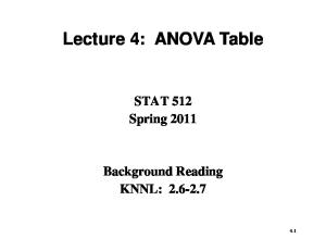
treatments were actually applied. This definition combines the results of several randomizations. For stocking rate and pasture evaluation trials we have that treatments are randomized to field units and the field units randomized to animal units, the latter randomization associating animal units with the field units. So the proposed definition would lead to the experimental unit for these trials being the field unit plus the associated animal unit. In this paper we propose a method for determining the ANOVA model and table to be used in analysing grazing trials that we believe facilitates determining whether valid error terms are available and what sources of variability contribute to these error terms. We advocate that one should derive this table at the design stage and use it as the basis for evaluating whether a proposed design has proper and adequate replication. In this, our objective is the same as that for the identification of the experimental units, but we achieve it without explicitly identifying them and without using the variation of experimental units to determine error terms. Not identifying the experimental unit avoids the ambiguity in its definition. Instead we describe the randomizations that have occurred. The method involves identifying (i) the factors associated with three sets of entities: the treatments, field units and animals and (ii) the field unit factor combinations to which the treatments are randomized and the animal factor combinations to which the field units are randomized. This information is then used to determine the lines or terms in the analysis of variance table and the proper error term for judging treatment differences is identified using their expected mean squares. In the next section we outline the proposed method. Then the method is applied to continuous grazing trials, rotational grazing trials, supplementary feeding trials, trials in which blocks correspond to different sites, unreplicated trials and trials involving repeated measurements over time. This paper is an extended version of Brien and Demétrio (1998). Method The procedure we will use to derive the analysis of variance table is illustrated in Figure 1. The first point to note about this method is that it begins with the identification of the observational unit which Federer (1975) defines to be ‘the smallest unit on which an observation is made’. An advantage of using the observational unit rather than the experimental unit is that for each response variable there is only one type of observational unit in an experiment whereas it is clear from Federer (1975) and the discussion above that there might be several different types of experimental unit. Thus, it should be easier to identify the observational unit. In general, for response variables measured on the animals, an animal or a group of animals is the observational unit; for response variables measured on the field units, a paddock, a plot or a quadrat is the observational unit. The crucial feature of the procedure is that, as well as categorizing the factors as fixed or random, the factors are also divided into sets or tiers as described by Brien (1983, 1989) according to their status in the randomization that was performed in designing the experiment. In grazing trials there are often three tiers, each tier consisting of the factors associated with one of the three sets of entities: the treatments, field units and animals. It is vital for this that all factors involved in the experiment are identified. One then uses the tiers to specify several structure formulae using the rules described in Table 1 of Brien (1983). Usually three structure formulae are required to describe grazing trials. The structure formulae encapsulate the nesting and crossing relationships between factors. In particular,

4

C.J. BRIEN AND C.G.B. DEMÉTRIO

A|B in a structure formula indicates that the factors A and B are crossed and A/B indicates that the factor B is nested within the factor A. Identify observational unit and factors

Categorize factors as fixed or random

Determine tiers

A

fi

d

Specify structure formulae

Derive terms, and their degrees of freedom, from the first structure formula (see Step 1, Table 1)

Derive expected mean squares for current formula; revise expected mean squares in ANOVA table (see Steps 4 and 5, Table 1)

Incorporate current terms into ANOVA table (see Steps 2 and 3, Table 1)

Derive terms, and their degrees of freedom, from the next structure formula (see Step 1, Table 1)

No

Last formula?

Yes

Stop

Figure 1 Procedure for deriving the analysis of variance table for an experiment Then for each structure formula in turn, extend the analysis table as illustrated in Figure 1 and detailed in Table 1: expand the formula to obtain the terms from it; derive the expected mean squares for these terms using standard rules; incorporate the terms, their degrees of freedom and expected mean squares into the analysis table. The process begins with the structure formula involving only factors whose levels are intrinsically associated with the observational units — terms involving

SPECIFYING THE ANOVA MODEL AND TABLE FOR GRAZING TRIALS

5

these factors make up the initial ANOVA table. This table is extended by incorporating the terms from the second structure formulae into it as described in Table 1. The extended ANOVA table is further extended by incorporating the terms from each of the other structure formulae until the terms from all structure formulae have been incorporated into the ANOVA table. The rules for expanding each structure formula are described in step 1 of Table 1 and are based on those given in Heiberger (1989). If the factors A and B are crossed (A|B in a formula), these rules lead to the terms A, B and A ×B being included in the analysis where A×B represents the interaction of the factors A and B. If factor B is nested within factor A (A/B in a formula), the standard rules lead to the terms A and B[A] being included in the analysis where B[A] represents the effects of B within the levels of A. As an example of using the rules for a more complicated formula we expand (A|B)/(C|D): A|B / C|D = A|B + C|D A B

b g b g b g b g

b

g

= A +B + A ¥B + C +D + C ¥D A B = A +B + A ¥B + C A B +D A B + C ¥D A B In this set of terms, the term C×D[A B] stands for the interaction between C and D nested within each combination of the levels of A and B; that is [A B] represents the combinations of A and B.

Table 1 Procedure for incorporating the terms from a formula into the analysis of variance table For each structure formula in turn, designate it as the current structure formula and carry out the steps in this table. Step 1

Procedure Expand the structure formula to produce a list of model terms using the following primary rules for structure formulae L and M: L / M = L + M fac L

bg

L| M = L + M + L ¥ M where fac L is the list of factors that occur in L, and L ¥ M = Â S ¥ T for all terms S in L and terms T in M. The following secondary rules for structure formulae L, N, P, Q and R deal with the handling of intermediate results in the expansion: N + P fac L = N fac L + P fac L

bg

b

g bg bg bg dP facbNg i facbLg = P facbL Ng P facbN g ¥ R facbQg = P ¥ R facbN Qg

b g

2

where fac L N is the combined list of the factors occurring in either L or N. Also work out the degrees of freedom for each term. Incorporate the model terms from the current structure formula. If the current formula is the first formula, which contains only unrandomized factors, list in the table all the model terms obtained from it. When incorporating terms from other than the first formula, place them indented

C.J. BRIEN AND C.G.B. DEMÉTRIO

3

4

5

6

under sources already in the ANOVA table with which they are confounded. All terms from the same formula will be indented so that they start at the same vertical position, there being a different starting position for the terms from each formula. Insert the degrees of freedom for each of the newly incorporated model terms. Model terms that arise in two consecutive formulae will not have a line entered for the formula incorporated last. When two model terms are totally aliased, such as can occur with fractional factorial experiments, one will be omitted from the analysis and a note of it made under the table. Add a Residual line for each source that had a model term incorporated under it in step 2, provided the Residual degrees of freedom are greater than zero. The number of Residual degrees of freedom is equal to the difference between those of the original source and the sum of the degrees of freedom of the terms incorporated under it. Where model terms have been incorporated under a source in the analysis as described in step 2, transfer the expected mean square from that source to each of the model terms incorporated under it and, if there is one, to its Residual line. Use standard rules to determine expected mean squares for model terms currently being incorporated as if these were the only terms in the model. For each model term being incorporated, add its expected mean square to that recorded for it in the analysis table after step 4.

In terms of performing the analysis in a statistics package, the notation we use for structure formulae corresponds to that used in p-Stat (Heiberger, 1989) and is similar to that used by Genstat (Payne, 1993); it has been chosen to fit with the most commonly used notations. Unfortunately many packages do not allow you to specify the analysis in terms of succinct structure formulae — most require that you specify a list of terms, although some allow the use of a factor crossing operator as a shorthand. Furthermore, there is currently no package that allows you to specify the analysis using three or more structure formulae as is required for the proposed method. So that the analysis can be performed using any package, we will provide a list of model terms for each analysis that will produce the set of sums of squares that consists of those for the lines with expected mean squares. That is, the derivation of the analysis of variance table will have to be done manually and the sums of squares added to it once they have been obtained using a package. Analyses for different grazing trials In this section we will discuss the analysis for both continuous and rotational grazing trials. In continuous grazing trials the field units are grazed without interruption. In rotational grazing trials the field units are grouped and each field unit within a group is grazed in turn by animals assigned to that group of units. We will use the generic term ‘plot’ to refer to a field unit in a grazing trial — a plot may be a small area of land or a whole paddock.

Continuous grazing in a randomized complete block design The design of these trials using a randomized complete block design generally involves the assignment of t treatments, possibly derived from several factors, to t plots in each of b blocks. Also, bt plots are randomized to the bta animals such that each plot receives a animals. A number of methods might be used for assigning the

SPECIFYING THE ANOVA MODEL AND TABLE FOR GRAZING TRIALS

7

animals to the plots (see for example, Roberts, 1975; ‘t Mannetje, Jones and Stobbs, 1976; Pimentel-Gomes et al., 1988). The method advocated by Roberts (1975) is to divide the animals into a homogeneous weight classes based on initial weight and to randomize the bt plots to the bt animals in each class. This method has the advantage that it avoids the risk of bias in estimating treatment effects associated with the method suggested by Pimentel-Gomes et al. (1988) and that an interaction between treatments and classes does not contribute to the error for treatment differences. Note that in the above discussion the plots are described as randomized to the animals rather than vice versa. This is because the number of animals is greater than the number of plots, except when only one animal is to be placed on a plot and then the number of animals will equal the number of plots. Consequently, plots in this randomization are analogous to treatments in a conventional randomization where the number of treatments is less than the number of units to which they are being applied. In practice, it is immaterial for such orthogonal designs whether the plots are randomized to the animals or vice versa. However, it would be important if a nonorthogonal design was used; this would only be necessary if the number of animals per class is not a multiple of bt, the number of plots. Generally, the use of nonorthogonal designs is not necessary as the number of weight classes and the number of animals per class is at the discretion of the experimenter. We will use the procedure outlined in Figure 1 to derive the analysis of variance for the experiment just described to either assess the proposed design or analyse results obtained with it. In specifying an analysis that reflects the randomization in such experiments it is crucial to recognize that they involve at least two randomizations: the randomization of the treatments to the plots and that of the plots to the animals. Analysis for an animal response variable. In this case the observational unit is an animal and, as in Brien (1983), one can identify three sets of factors, or tiers, associated with the bta observational units: unrandomized animal factors: randomized field factors: randomized treatment factors:

Classes, Animals Blocks, Plots Treatments

The tiers differ in the randomization status of their factors. Note that for any two factors from the same tier, the combinations of the levels of the factors that occur together is not the result of any of the randomization employed in the experiment. However, for the factors from different tiers, the randomization determines which combination of the levels of the factors from one tier occurs with a combination of the levels of the factors from another tier. For example, the block-plot combination that occurs with a particular animal-class combination is determined by the randomization, but the animal that occurs in a particular class is not. In general, the levels of the factors from one of the tiers will not have been randomized to the observational units and these factors are labelled unrandomized factors; a randomized factor is one whose levels have been randomized to the observational units. For the example, the factors Classes and Animals have not been randomized to the observational units, animals, and so are the unrandomized factors. The other two tiers of factors involve factors that were randomized to the observational units, one tier in the randomization of the plots to animals and the other in the randomization of the treatments to plots. It is necessary to have two tiers of

8

C.J. BRIEN AND C.G.B. DEMÉTRIO

randomized factors because the level of Treatments that occurs with a combination of the levels of Blocks and Plots is determined by randomization. On the other hand, the level of Plots that occurs with a level of Blocks is not determined by randomization. The structure formulae based on the three tiers are: Classes / Animals; Blocks / Plots; Treatments. Also, we will designate Blocks, Plots and Animals as random factors and Classes and Treatments as fixed factors. The basis we use to decide whether a factor is fixed or random is similar to that described by Robinson (1991) and Harville (1991). The factors Classes and Treatments are designated as fixed because we expect the effects for a term involving these factors to display systematic differences so that the population effects distribution would not be described adequately by a (normal) probability distribution. On the other hand we expect that the population distribution of effects for a term involving at least one of the random factors to be described at least approximately by a (normal) probability distribution. If this is thought to be unreasonable for Blocks in a particular experiment — for example, if a systematic trend in the response variable occurs across the blocks — Blocks should be designated as fixed also. While we believe this to be the appropriate basis for choosing whether a term is fixed and random, we recognise that others are in widespread use and note that any of these bases can be used with our proposed method of obtaining the analysis of variance table. We start the derivation of the full analysis of variance table with that based on the formula involving only unrandomized factors; performing steps 1, 2 and 5 results in the ANOVA table given in Table 2. Note that Animals[Classes] stands for Animals nested with Classes, that σ2A C is the variance component reflecting variability arising from different animals in the same weight class and that qC ψ is the contribution of

d i

the fixed term Classes to the expected mean squares. It is a quadratic form and will be the variance of the Classes population effects where ψ is a vector containing the expected values for the units — the algebraic expression for it is obtained by replacing the observations with their expected values in the formula for the Classes mean square. Table 2 Analysis of variance table for unrandomized factors from a continuous grazing trial Source df Expected mean squares Classes a −1 σ2A C +qC ψ Animals[Classes]

b g abbt − 1g

d i

σ2A C

Next the steps in Table 1 are performed for the second structure formula to extend Table 2 to Table 3. Step 1 yields the terms Blocks and Plots[Blocks] derived from the randomized field factors. In step 2, both Blocks and Plots[Blocks] are indented under Animals[Classes] because the bt block-plot combinations were randomized to the animals within a class so that Blocks and Plots[Blocks] is confounded with Animals[Classes]. Step 3 results in the inclusion of a Residual line under Animals[Classes] because there remains bt − 1 a − 1 degrees of freedom for Animals[Classes] after taking into account Blocks and Plots[Blocks]. Following step 4, the expected mean squares for Animals[Classes] in Table 2 are transferred to the Blocks, Plots[Blocks] and Residual lines in Table 3. Finally, as specified in step 5, the expected mean squares arising from just the terms incorporated at this step are

b

gb g

9

SPECIFYING THE ANOVA MODEL AND TABLE FOR GRAZING TRIALS

derived — they are aσP2 B + taσB2 for the Blocks line and aσP2 B for the Plots[Blocks] line where σP2 B is the variance component reflecting variability between plots within the same block and σB2 is the variance component reflecting the variability in overall block differences. Each of these expected mean squares is added to its line in the analysis table. Table 3 Analysis of variance table for unrandomized and randomized field factors from a continuous grazing trial Source df Expected mean squares Classes a −1 σ2A C +qC ψ Animals[Classes] Blocks Plots[Blocks] Residual

b g abbt − 1g bb - 1g bbt - 1g bbt − 1gba − 1g

d i

σ2A

C

+aσP2 B + taσB2

σ2A

C

+aσP2 B

σ2A

C

Lastly, the steps in Table 1 are performed for the third structure formula to add the term Treatments to Table 3 which yields the full analysis given in Table 4. In step 2, Treatments is indented under Plots[Blocks] because the randomization of treatments to plots within a block means that Treatments is confounded with Plots[Blocks]. In step 3, a Residual line has been included under Plots[Blocks] as there remains b − 1 t − 1 degrees of freedom for Plots[Blocks] after Treatments have been taken into account. In step 4, the expected mean square for Plots[Blocks] in Table 3 was transferred to Treatments and the Residual line. In step 5, qT ψ , the

b gb g

d i

contribution of Treatments to the expected mean squares, is added to the expected mean square for Treatments. Table 4 Full analysis of variance table for an animal response variable from a continuous grazing trial Source df Expected mean squares 2 Classes a −1 σA C +qC ψ Animals[Classes] Blocks Plots[Blocks] Treatments Residual Residual

b g abbt − 1g bb - 1g bbt - 1g bt - 1g bb - 1gbt - 1g bbt − 1gba − 1g

d i

σ2A

C

+aσP2 B + taσB2

σ2A

C

+aσP2 B

σ2A C

+aσP2 B

σ2A

+qT ψ

d i

C

In terms of assessing the design proposed for this trial, we see that the randomization of treatments to plots within blocks results in Treatments being confounded with Plots[Blocks] and the randomization of block-plot combinations to

C.J. BRIEN AND C.G.B. DEMÉTRIO

10

animals within classes results in Blocks and Plots[Blocks] being confounded with Animals[Classes]. The import of the confounding in this design is that Treatments differences, the effects of prime interest, are free of Classes and Blocks differences and it is evident from Table 4 that Treatments would be tested using the Residual for Plots[Blocks] — the expected mean squares for these two lines differ only in the quadratic form for Treatments so that the mean squares will be significantly different only if there are real differences between the treatments. Clearly, the Residual for Plots[Blocks] provides a valid error term for Treatments and so would be used for computing the standard error of a Treatment mean. Its expected mean square makes it clear that both animal and plot variation will contribute to its magnitude. Note that one might consider substituting the more familiar Treatments × Blocks for the Residual line for Plots[Blocks] in the above analysis because the two terms have the same degrees of freedom and sums of squares and so are apparently equivalent. However, this option should be avoided because they are not — they have different sources. The Residual line for Plots[Blocks] models the differences between plots within a block and represents a source of pure field unit variability; further, it is most likely to be a random term because Plots will almost certainly be designated as a random factor. On the other hand, Treatments × Blocks models the differential response of treatments in the different blocks and represents a source of interaction between field units and treatments; it may well be fixed because it is not unusual to have both Treatments and Blocks designated as fixed factors. The analysis presented here is based on the assumption that there is no interaction between blocks and treatments and so the term for it should not be included in the analysis table. However, if one was not prepared to make the assumption, the third structure formula could be modified to include it as per Step 4 of Table 1 in Brien (1983). The third structure formula would become Treatments | Blocks and the analysis would now include both Plots[Blocks] and Treatments × Blocks with these two terms being totally confounded. While a full analysis would include all the lines in Table 4, so that the confounding between terms is displayed in the ANOVA table, no statistical package is capable of producing this analysis. However, the analysis can be accomplished with only those sums of squares for the lines in Table 4 for which there are expected mean squares. For each expected mean square, identify a term that has the required degrees of freedom and sum of squares and include it in the list of terms to be fitted. In this case, five sums of squares are required and they could be obtained by fitting the following set of terms: Classes + Blocks + Treatments + Treatments × Blocks, the fifth sum of squares being the error sum of squares resulting from the fitting of these terms using a statistical package. Note that the fitted terms are being used merely for computational convenience in that, irrespective of whether or not they have been included in the ANOVA model and table for the experiment they nonetheless result in the correct sums of squares. For example, Treatments × Blocks is not a term included in Table 4 because we have assumed that Treatments and Blocks did not interact in the experiment. However, we include it in the list of terms to be fitted in obtaining the sums of squares because it provides the correct sums of squares for the Residual line for Plots[Blocks]. That is, we will interpret the resulting sum of squares as measuring plot and animal variability, not block-treatment interaction.

11

SPECIFYING THE ANOVA MODEL AND TABLE FOR GRAZING TRIALS

The analysis for one animal per plot can be derived from Table 4 by setting a = 1 throughout the table, removing any lines with zero degrees of freedom, and any occurrence of the factor Classes. This will have the effect of removing the line Classes and the last Residual line from the table. Also, if only the total (or mean) of the response variable taken over the animals on a plot is analyzed, the observational unit becomes a group of animals on a plot and the analysis is the same as for a single animal per plot with Group substituted for Animal. An important point that arises from the analysis in Table 4 is that σ2A C represents the variability between animals within classes and that there is no variance component corresponding to group differences. This is because the plots were randomized to the animals within a class and the differences between the groups of animals that end up on different plots is expected to be no greater than those arising from the different animals in each group and the different plots on which they graze. Put another way, everything else being equal — same plots, same treatments, same class — the groups of animals are not expected to be any more different than can be expected from the differences between animals within the groups. If this was thought to be unlikely — perhaps there are differences between the groups such as in handling and disease that arise during the conduct of the experiment — a variance component for Groups should be included even though this term is not justified by the randomization that was performed. The analysis of variance table is given in Table 5. Table 5 Analysis of variance table incorporating groups for an animal response variable from a continuous grazing trial Source df Expected mean squares 2 Classes a −1 sCG +qC ψ Groups Blocks Plots[Blocks] Treatments Residual Classes×Groups

b g bbt − 1g bb - 1g bbt - 1g bt - 1g bb - 1gbt - 1g bbt − 1gba − 1g

d i

s2CG +as2G +asP2 B + tasB2 s2CG +as2G +asP2 B s2CG

+as2G

+qT ψ

d i

+asP2 B

s2CG

There is little difference between Tables 4 and 5. Treatments would still be tested using the Residual for Plots[Blocks]. However, from Table 5 it is seen that group and plot differences contribute to this Residual whereas the corresponding Residual in Table 4 does not appear to include group differences. But group differences are seen to be implicitly included in σP2 B when it is recognized that the animals are in groups by virtue of being placed on the same plots and so any group differences are associated with plot differences. Table 5 has the advantage of making this explicit. Analysis for a field response variable. Suppose that a response variable is measured on q quadrats in each of bt plots and that the resulting data is to be

12

C.J. BRIEN AND C.G.B. DEMÉTRIO

analysed. The observational unit in this case is a quadrat. The factors describing the btq observational units can be divided into the following tiers: unrandomized field factors: randomized animal factors: randomized treatment factors:

Blocks, Plots, Quadrats Groups Treatments

Again, for any two factors from the same tier, the combinations of their levels that occur together is not the result of the randomization employed in the experiment, but for any two factors from different tiers it is. The factors Blocks, Plots and Quadrats are not randomized to the observational units, the quadrats, and so are innate to them. The animal factor that indexes quadrats is Groups, a group consisting of the a animals, each from a different class, on the same plot and there being bt groups altogether. Note that the factor Animal does not occur in this analysis because the response variable does not involve making observations on individual animals. The levels of this factor that occur on a particular quadrat are determined by the randomization of the field factors to the animal factors. The structure formulae based on the three tiers are: Blocks / Plots / Quadrats; Groups; Treatments. Also, we will designate Blocks, Plots, Quadrats and Groups as random factors and Treatments as a fixed factor. The full analysis of variance table derived using the steps outlined in Table 1 is given in Table 6. Note that the term Quadrats[Blocks Plots] represents the differences between quadrats within each block-plot combination. Also, this analysis is unusual in that the same animal term is confounded with two field terms: of the bt - 1 degrees of freedom for Groups, b − 1 are confounded with Blocks, while the remaining b t − 1 are confounded with Plots[Blocks]. This reflects the fact that there are different groups in different blocks and on different plots.

b

g

b g

b g

Table 6 Full analysis of variance table for a field response variable from a continuous grazing trial Source df Expected mean squares Blocks b -1 Groups b -1 s2Q BP +qsP2 B +qtsB2 +qs2G Plots[Blocks] Groups Treatments Residual Quadrats[Blocks Plots]

b g b g bbt - 1g bbt - 1g bt - 1g bb - 1gbt - 1g bt bq - 1g

s2Q BP +qsP2 B

+qs2G +qT ψ

s2Q BP +qsP2 B

+qs2G

d i

σ2Q BP

From Table 6 we see that the expected mean squares for Treatments and the Residual for Groups differ only in the quadratic form for Treatments. Hence the Residual for Groups provides a valid error for testing for Treatments effects and for computing the standard error of a Treatment mean. Also the expected mean square for the Residual makes it clear that the error for treatment differences involves

SPECIFYING THE ANOVA MODEL AND TABLE FOR GRAZING TRIALS

13

animal and plot variation. The four sums of squares for the analysis can be obtained by fitting the following set of terms: Blocks + Treatments + Treatments × Blocks and the analysis produced corresponds to that for a two-way classification with interaction and equal replication within the cells. The analysis for one quadrat per plot or a single value for the whole plot can be derived from Table 6 by setting q = 1, removing the Quadrats[Blocks Plots] line from the analysis and its variance component from the expected mean squares.

Rotational grazing in a randomized complete block design Duncalfe (1984) describes the use of rotational grazing experiments to reduce the error mean square and to increase the power of significance tests. Balanced against these advantages is that such experiments involve repeated measurements on the same animal over the rotations so that one needs to be particularly cautious in analysing them using the analysis of variance. It is not unusual for the assumptions underlying the analysis of repeated measurements designs to be unmet. We will present the analysis of variance to use provided that they are. As an example of a rotational grazing experiment, suppose we divide the experimental area into b blocks, each block into r paddocks and each paddock into t subpaddocks. Next, we assign t treatments, possibly derived from several factors, to the subpaddocks in each paddock and the r rotations to the r paddocks in a block. Also, we randomize the bt block-treatment combinations to the bta animals by dividing the animals into a homogeneous weight classes based on initial weight and randomizing the block-treatment combinations to the bt animals in each class — each combination receives a animals. There are two randomizations that have to be taken into account in deriving the analysis: the randomization of block-treatment combinations to animals and that of treatment-rotation combinations to the field units. Analysis for an animal response variable. The analysis of variance for the animal response variable from a rotational grazing trial is derived using the procedure outlined in Figure 1. The observational unit is an animal and one can identify three sets of factors, or tiers, associated with the btar observational units: unrandomized animal factors: randomized field factors: randomized treatment factors:

Classes, Animals, Rotations Blocks, Paddocks, SubPaddocks Blocks, Treatments, Rotations

Again, for any two factors from the same tier, the combinations of their levels that occur together is not the result of the randomization employed in the experiment, but for any two factors from different tiers it is. However, this is an unusual example because the factors Blocks and Rotations occur in two tiers. It is necessary to include Rotations in the unrandomized animal factors so that each combination of the levels of the lowest tier’s factors occur only once; it is also included in the randomized treatment factors because it was randomized to the Paddocks. Blocks is clearly a factor innate to the field units and is required because the Paddocks are nested within them; however, the block-treatment combinations are randomized to the animals and so Blocks must be included in the randomized treatment factors also. This is different to the situation with continuous grazing trials where Blocks should not be included in the randomized treatment factors as it was not involved in

14

C.J. BRIEN AND C.G.B. DEMÉTRIO

the randomization of treatments. Its inclusion in the third structure formula is optional, depending on the assumptions one is prepared to make. The structure formulae based on the three tiers are: ( Classes / Animals ) | Rotations; Blocks / Paddocks / SubPaddocks; Treatments | Blocks | Rotations. An alternative structure formula for the randomized treatment factors is Treatments | (Blocks + Rotations) as this would include only the terms that were involved in the randomizations. However, this makes little difference to the analysis and so we use the original formula. We will designate Blocks, Paddocks, SubPaddocks and Animals as random factors and Classes, Treatments and Rotations as fixed factors. This is not the only division of the factors into fixed and random; for example, it can be envisaged that in some circumstances Rotations would be more appropriately designated a random factor. The full analysis of variance table derived using the steps outlined in Table 1 is given in Table 7. In this analysis some field terms are confounded with two animal terms: r - 1 of the degrees of freedom for the term Paddocks[Blocks] are confounded with Rotations, while the remaining b - 1 r - 1 degrees of freedom are confounded with

b g

b gb g

Animals × Rotations[Classes]. SubPaddocks[Blocks Paddocks] is similarly confounded with two animal terms. Also, it differs from previous analyses by including Treatments × Blocks and other interactions with Blocks. The term is included in this case because it was randomized to animals. It can be seen from the expected mean squares in Table 7 that of the terms involving Treatments, only Treatments and Treatments × Rotations have valid error terms: Treatments × Blocks and Treatments × Blocks × Rotations, respectively. These error terms involve both animal and subpaddock variability. There is no valid error for Rotations differences because there is no mean square that includes a variance component for Paddocks[Blocks] but not a component for Rotations — the two are inseparable. Similarly, all interactions involving Blocks cannot be tested because their effects cannot be separated from some source of field-unit variability. The ten sums of squares for the analysis can be obtained by fitting the following terms: Classes + Rotations + Classes × Rotations + Treatments + Blocks + Treatments × Blocks + Blocks × Classes + Treatments × Classes + Blocks × Treatments × Classes + Blocks × Rotations + Treatments × Rotations + Treatments × Blocks × Rotations + Blocks × Rotations × Classes + Treatments × Rotations × Classes. The resulting analysis is that for a four-way classification with all main effects and interactions between the four factors Classes, Rotations, Treatments and Blocks, except for the four-factor interaction. However, to obtain the Residual sums of squares for the analysis presented in Table 7 some sums of squares have to be combined. To obtain the Residual sums of squares for Animals[Classes] combine those for the terms Blocks × Classes, Treatments × Classes and Treatments × Blocks × Classes. Similarly, the Residual sums of squares for Animals × Rotations[Classes] is formed by combining those for Blocks × Rotations × Classes, Treatments × Rotations × Classes and the Error.

15

SPECIFYING THE ANOVA MODEL AND TABLE FOR GRAZING TRIALS

Source

Table 7 Full analysis of variance table for an animal response variable from a rotational grazing trial df Expected mean squares 2 2 2 σ AR C σ A C σS2 BP σP2 B σB2 σ2TBR σ2TB σBR

Classes Rotations Paddocks [Blocks] Classes × Rotations Animals[Classes] Blocks SubPaddocks[Blocks Paddocks] Treatments Treatments × Blocks Residual Animals × Rotations[Classes] Paddocks [Blocks] Blocks × Rotations SubPaddocks[Blocks Paddocks] Treatments × Rotations Treatments × Blocks × Rotations Residual

qC ψ

ba − 1g br - 1g

1

br - 1g ba − 1gbr − 1g abbt − 1g bb - 1g bbt - 1g

1

1

r

a

bt - 1g bt - 1gbb - 1g ba − 1gbbt − 1g abbt − 1gbr − 1g bb - 1gbr - 1g bb - 1gbr - 1g bbt - 1gbr - 1g bt - 1gbr - 1g bt - 1gbb - 1gbr - 1g ba − 1gbbt − 1gbr − 1g

1 1

r r

a a

1

r

d i

r

a

ra

ta qR ψ

d i dψ i

a

qCR

1

1

a

1 1

a a

1

ra

ra

tra

a

ra

a a

ra ra

a

a a

ta

qT ψ

d i

ta

qTR ψ

d i

C.J. BRIEN AND C.G.B. DEMÉTRIO

16

The analysis for measurements pooled over the rotations can be derived from that in Table 7 by setting r = 1 throughout the table and removing all terms with zero degrees of freedom from the analysis and expected mean squares. The analysis for a single animal per subpaddock can be obtained by setting a = 1 throughout the table and removing all terms with zero degrees of freedom from the analysis and expected mean squares. This will have the effect of removing the factor Classes from the analysis so that the lines for Classes, Classes × Rotations and the two Residual lines would be omitted from the analysis. Analysis for a field response variable. For a field response variable measured on q quadrats in each subpaddock the observational unit is a quadrat. The factors describing the btrq observational units can be divided into the following tiers: unrandomized field factors: randomized animal factors: randomized treatment factors:

Blocks, Paddocks, SubPaddocks, Quadrats Herds, Rotations Blocks, Treatments, Rotations

The structure formulae based on the three tiers are: Blocks / Paddocks / SubPaddocks / Quadrats; Herds | Rotations; Treatments | Blocks | Rotations. Again, an alternative structure formula for the randomized treatment factors is Treatments | (Blocks + Rotations). We will designate Blocks, Paddocks, SubPaddocks and Animals as random factors and Classes, Treatments and Rotations as fixed factors. The full analysis of variance table derived using the steps outlined in Table 1 is given in Table 8. The valid error terms for this analysis are the same as those for the analysis of an animal response variable, as are the lines that do not have valid error terms. The eight sums of squares for the analysis can be obtained by fitting the following terms: Blocks + Rotations + Blocks × Rotations + Treatments + Blocks × Treatments + Rotations × Treatments + Blocks × Rotations × Treatments. The resulting analysis is that for a three-way classification with equally replicated cells. The analysis for measurements pooled over the rotations can be derived from that in Table 8 by setting r = 1 throughout the table and removing all terms with zero degrees of freedom from the analysis and expected mean squares. The analysis for one quadrat per plot or a single value for the whole plot can be derived from Table 8 by setting q = 1 throughout the table and removing all terms with zero degrees of freedom from the analysis and expected mean squares. This will have the effect of removing the Quadrats[Blocks Paddocks SubPaddocks] line from the analysis and variance component from the expected mean squares.

17

SPECIFYING THE ANOVA MODEL AND TABLE FOR GRAZING TRIALS

Source

Table 8 Full analysis of variance table for a field response variable from a rotational grazing trial df Expected mean squares 2 2 2 2 2 σQ BPS σS BP σP B σB2 σHR σH2 σ2TBR σ2TB σBR

Blocks Herds Paddocks [Blocks] Rotations Herds × Rotations Blocks × Rotations SubPaddocks[Blocks Paddocks] Herds Treatments Treatments × Blocks Herds×Rotations Treatments × Rotations Treatments × Blocks × Rotations Quadrats[Blocks Paddocks SubPaddocks]

bb - 1g bb - 1g bbr - 1g br - 1g bb - 1gbr - 1g bb - 1gbr - 1g br bt - 1g bbt - 1g bt - 1g bt - 1gbb - 1g bbt - 1gbr - 1g bt - 1gbr - 1g bt - 1gbb - 1gbr - 1g btr bq - 1g

q

rq

rq

1

q

rq

q

q

tq qR ψ

1

q

rq

q

q

tq qCR ψ

1 1

q q

q q

1 1

q q

q q

rq rq

q

q q q q

rq

d i

q

1

trq

tq qC ψ

1

d i d i

rq rq

qT ψ

d i

qTR ψ

d i

18

C.J. BRIEN AND C.G.B. DEMÉTRIO

Supplementary feeding trials Four types of supplementary feeding trials, three of which are grazing trials, are examined. Each of these trials allows the researcher to obtain different information from them and this needs to be borne in mind when deciding the type of trial to employ. These trials were outlined by a referee of Brien and Demétrio (1998). In all trials that involve pens we will refer to pens as feedpens and presume that these are formed into rows. We do this for notational convenience so that all the factors involved will begin with a different initial letter. In reality, the sets of feedpens may be formed into groups without being in different rows, or may not be grouped at all. Also, it will be presumed that wherever possible the animals have been divided into homogeneous weight classes based on initial weight as in the continuous grazing trial. In all trials there will be t treatments, these being the different supplements. For each type of trial we outline one scenario for the blocking of the feedpens, animals and plots, recognizing that each is just one of many ways of blocking these units in these trials. We will present only the analyses for an animal response variable. Animals in feedpens throughout. Suppose that there are bta animals divided into a homogeneous initial-weight classes and bt feedpens are arranged in b rows. The bt feedpens are randomized to the bt animals in each class and the t treatments are randomized to the t feedpens in each row. All animals receive a basal diet plus their assigned supplement. The observational unit is an animal and one can identify three sets of factors, or tiers, associated with the bta observational units: unrandomized animal factors: randomized pen factors: randomized treatment factors:

Classes, Animals Rows, Feedpens Treatments

The structure formulae based on the three tiers are: Classes / Animals; Rows / Feedpens; Treatments. We will designate Animals and Feedpens as random factors and Classes, Rows and Treatments as fixed factors. The full analysis of variance table is given in Table 9. This analysis parallels that for the continuous grazing trial with Feedpens and Rows in this analysis replacing Plots and Blocks in the analysis for the continuous grazing trial. Table 9 Full analysis of variance table for a supplementary feed trial in which the animals are fed in pens throughout Source df Expected mean squares a -1 Classes s2A C +qC ψ Animals[Classes] Rows Feedpens[Rows] Treatments Residual Residual

b g abbt - 1g bb - 1g bbt - 1g

bt - 1g bb - 1gbt - 1g ba - 1gbbt - 1g

c h

s2A C +as2F

R

+qR ψ

s2A C +as2F

R

+qT ψ

s2A C +as2F R s2A C

c h

c h

19

SPECIFYING THE ANOVA MODEL AND TABLE FOR GRAZING TRIALS

From the expected mean squares it is clear that all lines have valid error terms. In particular, the Residual for Feedpens[Rows] will be used to test the Treatments term — both animal and feedpen variability contribute to this Residual. The five sums of squares for the analysis can be obtained by fitted the following terms: Classes + Rows + Treatments + Rows × Treatments. The analysis for the case when there is only one animal per pen can be obtained from Table 9 by setting a = 1 throughout the table, and removing the factor Classes and all terms with zero degrees of freedom from the analysis. Single plot, supplement in feedpens with several animals. In this type of trial animals common graze the one plot as a single herd throughout, except when mustered daily to be brought into feedpens when g animals are put into each feedpen for supplement feeding. There are ta feedpens arranged in t rows and the t treatments are randomized to the t feedpens in each row. The animals are divided into a homogeneous initial-weight classes and each of these classes is further subdivided into g groups so that altogether there are ag groups each comprised of t animals. The a rows are randomized to the a classes and the t feedpens in a row are randomly assigned to the t animals in each of the g groups. The observational unit is an animal and one can identify three sets of factors, or tiers, associated with the ta observational units: unrandomized animal factors: randomized pen factors: randomized treatment factors:

Classes, Groups, Animals Rows, Feedpens Treatments

The structure formulae based on the three tiers are: Classes / Groups / Animals; Rows / Feedpens; Treatments. We will designate Animals and Feedpens as random factors and Classes, Groups, Rows and Treatments as fixed factors. The full analysis of variance table is given in Table 10. Table 10 Full analysis of variance table for a supplementary feed trial in which the animals common graze a single plot Source df Expected mean squares a -1 Classes a -1 Rows s2A C +gs2F R +qR +C ψ Groups[Classes] Animals[Classes Groups] Feedpens[Rows] Treatments Residual Residual

b g b g abg - 1g ag bt - 1g abt - 1g

bt - 1g ba - 1gbt - 1g abg - 1gbt - 1g

s2A C +gs2F R +qG C

c h cψ h

s2A C +gs2F R +qT ψ

c h

s2A C

+gs2F R

s2A C

From the expected mean squares it is clear that Treatments has a valid error term, the Residual for Feedpens[Rows] — both animal and feedpen variability contribute to this Residual. The five sums of squares for the analysis can be obtained by fitted the following terms:

20

C.J. BRIEN AND C.G.B. DEMÉTRIO

Classes + Groups[Classes] + Treatments + Classes × Treatments. The analysis for the case when animal are individually fed in pens can be obtained from Table 10 by setting g = 1 throughout the table, and removing the factor Groups and all terms with zero degrees of freedom from the analysis. Several plots, supplement in individual feedpens. The randomization of the plots to the animals in this type of trial is the same as the continuous grazing trial. The t treatments are randomized to t plots in each of b blocks. Also, the animals are divided into a homogeneous initial-weight classes and the bt plots are randomized to the bt animals in each class so that each plot receives a animals. There are also a rows each consisting of bt feedpens. The a rows are randomized to the a classes and the bt feedpens in a row are randomized to the bt animals in the same class. The observational unit is an animal and one can identify four sets of factors, or tiers, associated with the ta observational units: unrandomized animal factors: randomized pen factors: randomized field factors: randomized treatment factors:

Classes, Animals Rows, Feedpens Blocks, Plots Treatments

The structure formulae based on the four tiers are: Classes / Animals; Rows / Feedpens; Blocks/Plots; Treatments. We will designate Animals, Feedpens, Plots and Blocks as random factors and Classes, Rows and Treatments as fixed factors. The full analysis of variance table is given in Table 11. Table 11 Full analysis of variance table for a supplementary feed trial in which the animals are divided between several plots and fed in feedpens Source df Expected mean squares Classes a −1 a -1 Rows s2A C +sF2 R +qR +C ψ Animals[Classes] Feedpens[Rows] Blocks Plots[Blocks] Treatments Residual Residual

b g b g abbt − 1g abbt - 1g bb - 1g bbt - 1g bt - 1g bb - 1gbt - 1g bbt − 1gba − 1g

c h

s2A C +sF2

R

+asP2

B

+tas2B

s2A C + sF2 R

+asP2

B

+qT ψ

s2A C + sF2 R

+asP2

B

s2A C

+

c h

sF2 R

From the expected mean squares it is clear that Treatments has a valid error term, the Residual for Plots[Blocks] — the animal, feedpen and plot variability contributes to this Residual. The five sums of squares for the analysis can be obtained by fitted the following terms: Rows + Blocks + Treatments + Treatments × Blocks.

21

SPECIFYING THE ANOVA MODEL AND TABLE FOR GRAZING TRIALS

Several plots, supplement in plots. This type of trial is just a continuous grazing trial in which the t treatments happen to be the t supplements which are fed to the animals in a plot. Sites as blocks Sometimes the blocks in the randomized complete block design used to randomize the treatments to the plots may correspond to very different sites, in which case as ‘t Mannetje, Jones and Stobbs (1976) point out, it is desirable to allow for the testing for site by treatment interactions. In order to do this it will be necessary to use a generalized randomized complete block design in which the treatments are replicated at each site. For example a continuous grazing trial is to be conducted in which t treatments, possibly derived from several factors, are completely randomized to the tr plots at each of s sites so that each treatment occurs on r plots at a site. Also, str plots are randomized to stra animals such that each plot receives a animals. We present only the analysis for an animal response variable. The observational unit is an animal and one can identify three sets of factors, or tiers, associated with the stra observational units: unrandomized animal factors: randomized field factors: randomized treatment factors:

Animals Sites, Plots Treatments

The structure formulae based on the three tiers are: Animals; Sites / Plots; Treatments | Sites. Note that Sites is included in the last structure formula because of the interest in the interaction between treatments and sites. Also, we will designate Plots and Animals as random factors and Sites and Treatments as fixed factors. Sites is being regarded as a fixed factor here, but it may be more appropriate to designate it as a random factor depending on whether it is thought that the population distribution of the effects of a term involving Sites can be approximated by a (normal) probability distribution. The full analysis of variance table is given in Table 12. Table 12 Full analysis of variance table for an animal response variable from a continuous grazing trial involving sites Source df Expected mean squares Animals stra - 1 Sites s -1 σ2A +aσP2 S +qS ψ

b

Plots[Sites] Treatments Treatments × Sites Residual Residual

g

b g sbtr - 1g bt - 1g bt - 1gbs - 1g st br - 1g str ba - 1g

d i

σ2A

+aσP2 S +qT ψ

σ2A

+aσP2 S

σ2A

+aσP2 S

d i + q dψ i TS

s 2A

From the expected mean squares it is clear that all lines have valid error terms. In particular, the Residual for Plots[Sites] will be used to test the Treatments, Sites and Treatments × Sites terms — both animal and plot within site variability contribute

22

C.J. BRIEN AND C.G.B. DEMÉTRIO

to this Residual. The five sums of squares for the analysis can be obtained by fitted the following terms: Sites + Treatments + Treatments × Sites + Plots[Treatments Sites]. The analysis for the case when the treatments are not replicated at each site is obtained from Table 12 by setting r = 1 throughout the table and removing all terms with zero degrees of freedom from the analysis. This has the effect of removing the Residual for Plots[Sites] from the analysis leaving no source that is suitable for testing either the Treatments or the Treatments × Sites terms. Of course, if we can be sure that there is little or no Treatments × Sites interaction, this source can be designated a Residual and the quadratic form in its expected mean square removed. Under these circumstances, the resulting Residual can be used to test for the Treatments term.

Improperly replicated trials Continuous grazing trial. Suppose that a continuous grazing trial is to be conducted, but that there is only one paddock for each treatment. Also, to illustrate what happens when animals of more than one type are placed in the same paddock, suppose that ta animals of each sex are to be used. The t paddocks are to be randomized to the ta animals from each sex completely at random such that a animals of each sex are assigned to each paddock. We present only the analysis for an animal response variable. The observational unit is an animal and one can identify three sets of factors, or tiers, associated with the 2 ta observational units: unrandomized animal factors: randomized field factors: randomized treatment factors:

Sex, Animals Paddocks Treatments

The structure formulae based on the three tiers are: Sex / Animals; Paddocks; Treatments | Sex. Note that Sex is included in the last structure formula as the investigator will be interested in whether there is an interaction between Treatments and Sex. Also, we will designate Paddocks and Animals as random factors and Sex and Treatments as fixed factors. The full analysis of variance table is given in Table 13. Table 13 Full analysis of variance table for an animal response variable from an improperly replicated continuous grazing trial involving sex Source df Expected mean squares Sex 1 σ2A S +qS ψ

d i

Animals[Sex] Paddocks Treatments Treatments × Sex Residual

b

g

2 ta − 1 t -1

b g bt - 1g bt - 1g 2t ba − 1g

σ2A

S

σ2A

S

σ2A S

+2aσP2

+qT ψ

d i + q dψ i TS

23

SPECIFYING THE ANOVA MODEL AND TABLE FOR GRAZING TRIALS

In terms of evaluating the design employed in this trial, we see that the randomization of treatments to plots results in Treatments being confounded with Paddocks and the randomization of paddocks to animals within each sex results in Paddocks being confounded with Animals[Sex]. Hence, Treatments differences are free of Sex differences. However, it is clear from the expected mean squares in Table 13 that a valid error for testing treatment differences is not available because there is no term other than Treatments whose expected mean square includes the variance component for paddocks. This means that the overall treatment differences cannot be separated from paddock differences — they are totally confounded with each other. Consequently, the trial suffers from the defect that any difference in the treatment means might be due to paddock rather than treatment differences. Inferences about overall differences between the treatments require further information or assumptions that are difficult to justify. For example one would need to know that for a particular trial there is very little paddock variability s 2P ≈ 0 or one

d

i

might be prepared to argue that based on experience the differences between the treatments means are large enough to be unquestionably due to the treatments. On the other hand, the Residual for Animals[Sex] provides an error for testing the Treatments × Sex interaction. The four sums of squares for the analysis can be obtained by fitting the following terms: Sex + Treatments + Treatments × Sex. The resulting analysis is that for the two-way classification with interaction and equal replication within the cells. If this analysis cannot be justified, the problem will have to be rectified. Generally such problems result from a lack of suitable replication — in this case the treatments need to be replicated by applying each of them to several paddocks. The analysis for the case when all animals are of the same sex can be derived from Table 13 by removing the lines for Sex and Treatments × Sex, changing Animals[Sex] to Animals and leaving the twos out of the degrees of freedom. Rotational grazing trial. As ‘t Mannetje, Jones and Stobbs (1976) note, one way to reduce herd size in grazing trials is to use a single herd to graze the replicates of each treatment in turn. For example, suppose that tr combinations of t treatments and r rotations are applied completely at random to tr paddocks so that each treatment-rotation combination occurs on one paddock. Also, the t treatments are assigned completely at random to ta animals so that each treatment is assigned to a animals. We present only the analysis for an animal response variable. The observational unit is an animal during a rotation and one can identify three sets of factors, or tiers, associated with the ar observational units: unrandomized animal factors: randomized field factors: randomized treatment factors:

Animals, Rotations Paddocks Treatments, Rotations

The structure formulae based on the three tiers are: Animals | Rotations; Paddocks; Treatments | Rotations. We will designate Paddocks and Animals as random factors and Treatments and Rotations as fixed factors. The full analysis of

24

C.J. BRIEN AND C.G.B. DEMÉTRIO

variance is given in Table 14. The five sums of squares for the analysis can be obtained by fitting the following terms: Treatments + Animals[Treatments] + Rotations + Treatments × Rotations. The resulting analysis is analogous to a ‘split-plot-in-time’ when the whole plot treatments are arranged according to a completely randomized design. Table 14 Full analysis of variance table for an animal response variable from an improperly replicated rotational grazing trial Source df Expected mean squares Animals ta - 1 Paddocks t -1 Treatments t -1 s 2AR +rs 2A +as 2P +qT ψ

b

g

b g

b g

b g

Residual

t a -1

Rotations Paddocks Animals×Rotations Paddocks Treatments×Rotations Residual

br - 1g br - 1g bta - 1gbr - 1g bt - 1gbr - 1g bt - 1gbr - 1g t ba - 1gbr - 1g

d i

s 2AR

+rs 2A

qR ψ

d i

s 2AR

+as 2P

s 2AR

+as 2P +qTR ψ

d i

s 2AR

b g

In this analysis the tr - 1 degrees of freedom for paddocks are spread across the three terms arising from the unrandomized animal factors. The problem with this trial is the same as in the improperly replicated continuous grazing trial — the overall treatment differences cannot be separated from paddock differences and so inferences about overall differences between the treatments requires further information or assumptions.

Repeated measurements over time Repeated measurements experiments over time involve the repeated observation of animal(s) or a field unit at successive times without changing the experimental setup. We present the analysis of variance for the special case of when it can be assumed that there is equal covariance between the observations from different times — if this assumption is not met alternative analyses must be used. Generally, the analysis of variance for repeated measurements experiments over time is obtained by adding a factor for time to the experimental unit, then introducing it into each structure formula and designating it as crossed with the other factors in the formula. For example, suppose that the experiment involving sites had measurements taken on each animal once a week for w weeks and these were to be analysed using analysis of variance.

25

SPECIFYING THE ANOVA MODEL AND TABLE FOR GRAZING TRIALS

Table 15 Full analysis of variance table for an animal response variable from a continuous grazing trial involving sites and weeks Source df Expected mean squares Animals stra - 1 2 2 2 Sites s -1 σ2AW +aσPW S + wσ A + awσP S +qS ψ

b

Plots[Sites] Treatments

g b g sbtr - 1g

bt - 1g bt - 1gbs - 1g st br - 1g

Treatments × Sites Residual Residual Weeks Animals × Weeks Sites × Weeks Plots × Weeks[Sites] Treatments × Weeks Treatments × Sites × Weeks Residual Residual

d i

b g

str a - 1

bw - 1g bstra - 1gbw - 1g bs - 1gbw - 1g sbtr - 1gbw - 1g bt - 1gbw - 1g bt - 1gbs - 1gbw - 1g st br - 1gbw - 1g str ba - 1gbw - 1g

2 σ2AW +aσPW

S

+ wσ2A +awσP2 S +qT ψ

σ2AW

2 +aσPW S

+ wσ2A

+awσP2 S

σ2AW

2 +aσPW S

+ wσ2A

+awσP2 S

d i + q dψ i TS

+ws 2A

s 2AW 2 σ2AW +aσPW

S

+qW ψ

2 σ2AW +aσPW

S

+qSW ψ

2 σ2AW +aσPW

S

+qTW ψ

2 σ2AW +aσPW

S

+qTSW

2 σ2AW +aσPW

S

s 2AW

d i d i

d i dψ i

C.J. BRIEN AND C.G.B. DEMÉTRIO

26

The observational unit is an animal in a week and one can identify three sets of factors, or tiers, associated with the straw observational units: unrandomized animal factors: randomized field factors: randomized treatment factors:

Animals, Weeks Sites, Plots Treatments

The structure formulae based on the three tiers are: Animals | Weeks; ( Sites / Plots ) | Weeks; Treatments | Sites | Weeks. We will designate Plots and Animals as random factors and Weeks, Sites and Treatments as fixed factors, although it is possible that in some experiments Weeks and/or Sites are better regarded as random factors. The full analysis of variance table is given in Table 15. The 11 sums of squares for the analysis can be obtained by fitting the terms Sites + Treatments + Sites × Treatments + Plots[Sites Treatments] + Animals[Sites Treatments Plots] + Weeks + Plots × Weeks[Sites Treatments]. This analysis is analogous to a ‘split-plot-in-time’ with the main plot forming a twoway classification with equal replication. The comments that apply to this analysis are similar to those given for Table 12. Conclusions We have demonstrated for continuous grazing trials how to produce analysis of variance tables that we believe facilitate determining whether valid error terms are available and what sources of variability contribute to these error terms. They do this because they show the confounding between terms which summarizes the results of the randomization in an experiment, since a particular randomization can be characterised as confounding particular terms with certain other terms. They, unlike a traditional table, exhibit this confounding by including a separate term for each of two confounded terms — only one of the terms would be included in a traditional table. For this to happen all factors involved in the experiment must be identified so that every source of variation will be explicitly incorporated in the analysis table. In addition, the factors need to be divided into tiers according to how they were randomized and the analysis of variance table derived from them in stages corresponding to the randomizations. Three tiers are required for the experiments presented here because they involve two randomizations: the randomization of treatments to field units and that of field units to animals. The first of these confounds treatment and field unit terms; the latter confounds field unit and animal terms, and consequently treatment and animal terms. Also, the expected mean squares are synthesized stage-by-stage so that one can see how the randomization affects which sources of variation contribute to the expected mean squares for a particular line. In particular, the expected mean square of an error term for testing a treatment term will always be the synthesis of both animal and field sources of variation. An advantage of our method is that there are separate terms in the analysis of variance table for every source of field differences and every source of animal differences and so it is much less likely that a source of variation will be accidentally overlooked. This makes it particularly useful as a basis for evaluating designs for grazing trials where one wants to use a skeleton ANOVA table to determine (i) which terms are confounded as a result of the factors and randomization incorporated into

SPECIFYING THE MODEL AND ANOVA TABLE FOR GRAZING TRIALS

27

the proposed design, (ii) whether a valid error term will be available for testing effects of interest because the replication is proper, and (iii) what components of variability will affect treatment differences which, with estimates of the magnitudes of these components, will allow an estimate of the magnitude of the error term. An important issue in designing all types of grazing trials is whether proper replication has been incorporated. However, saying ‘the experimental unit in a grazing trial is not properly replicated’ often meets with the response: ‘but I have several animals for each treatment!’. Further a traditional ANOVA table often does not alert one to the problem because they do not necessarily include terms for all the sources of variation that might occur in the experiment. For example, the traditional analysis for the improperly replicated trial in this paper would be a standard two-way analysis of variance with just the terms Classes, Treatments and Error, the latter being thought of as Classes × Treatments interaction — no Plots or Classes[Animals] terms. There is no clue in this analysis of any problem. The method outlined in the paper automatically reveals in a particularly clear manner when there is improper replication in a grazing trial. It shows up explicitly in the analysis of variance table as ‘treatments’ and ‘plots’ being totally confounded with each other so that it is impossible to obtain an error term for testing for treatment differences because any term that includes plot variability is also contaminated by treatment differences. As was pointed out for the improperly replicated grazing trial, inferences about overall treatment differences require further information or assumptions that may be difficult to justify. We feel that the grazing researcher will much more readily appreciate the limitations of such trials when it is said that ‘treatments’ and ‘plots’ are totally confounded because it concentrates on the repercussions of the problem. On the other hand stating that the replication is improper centres uninformatively on the origin of the problem and researchers appear to have at times not appreciated the implications of this statement. A bonus of the use of the proposed method is that the randomization employed in the experiment is recorded in the analysis of variance table in the form of the confounding between terms. If one does want to determine the experimental units(s) for an experiment, this information is exactly what is needed. So our method will assist in identifying the experimental unit(s). Acknowledgments We would like to thank the Centre for Industrial and Applied Mathematics, University of South Australia and CAPES, Brasil for their assistance in making possible Dr. C. Demétrio’s visit to Adelaide to work on this paper. Also, we are grateful to the referees for many comments that helped to greatly clarify and improve the paper. In particular, one of the referees provided us with description of different supplementary feeding trials that stimulated us to include their analysis in this paper. References Beattie, A.W., and Alexander, G.I. (1973). Design of field experiments. In Manual of Techniques for Field Investigations with Beef Cattle , edited by Alexander, G.I. CSIRO: Canberra, 8.1–8.24. Blight, G.W. and Pepper, P.M. (1982). Identification of the unit in experiments on supplementary feeding of beef cattle grazing native pasture. Proceedings of the Australian Society for Animal Production , 14, 297–300.

C.J. BRIEN AND C.G.B. DEMÉTRIO

28

Blight, G.W. and Pepper, P.M. (1984). Choosing the experimental unit in grazing trials: Hobson’s Choice? paper presented at the 7th Australian Statistical Conference. Bransby, D.I. (1989). Compromises in the design and conduct of grazing experiments. In Grazing Research: design, methodology, and analysis , edited by Marten, G.C. Crop Science Society of America Special publication, 16, 53– 67. Crop Science Society of America and American Society of Agronomy: Madison. Brien, C.J. (1983). Analysis of variance tables based on experimental structure. Biometrics, 39, 53-59. Brien, C.J. (1989). A model comparison approach to linear models. Utilitas Mathematica, 36, 225-254. Brien, C.J. and Demétrio, C.G.B. (1998) Using the randomization in specifying the ANOVA model and table for properly and improperly replicated grazing trials. manuscript submitted. Brown, M.A. and Waller, S.S. (1986). The impact of experimental design on the application of grazing research results — an exposition. Journal of Range Management, 39, 197–200. Conniffe, D. (1976). A comparison of between and within herd variance in grazing experiments. Irish Journal of Agricultural Research , 15, 39–46. Drane, J.W. (1989). Compromises and statistical designs for grazing experiments. In Grazing research: design, methodology, and analysis , edited by Marten, G.C. Crop Science Society of America Special publication, 16, 69–83. Crop Science Society of America and American Society of Agronomy: Madison. Duncalfe, F. (1984). In Blight, G.W. Experimental design in cattle research when resources are limiting. Proceedings of the Australian Society for Animal Production, 15, 52–65. Federer, W. T. (1975). The misunderstood split plot. In Applied Statistics, edited by R. P. Gupta, 9–39. North Holland: Amsterdam. Harville, D.A. (1991). Contribution to the discussion of a paper by G.K. Robinson. Statistical Science, 6, 35-39. Heiberger, R.M. (1989). Computation for the analysis of designed experiments . Wiley: New York. Moule, G.R. (1965). Field investigations with sheep: a manual of techniques . CSIRO: Australia. Payne, R.W., Lane, P.W., Digby, P.G.N., Harding, S.A., Leech, P.K., Morgan, G.W., Todd, A.D., Thompson, R., Tunnicliffe Wilson, G., Welham, S.J. and White, R.P. (1993) Genstat 5 Release 3 Reference Manual . Oxford University Press: Oxford. Petersen, R.G. (1994). Agricultural Field Experiments: Design and Analysis. Dekker: New York. Pimentel-Gomes, F., Nunes, S.G., Gomes, M. B. and Curvo, J.B.E. (1988). Modificação na análise da variância de ensaios de pastejo com bovinos, considerando os blocos como animais. Pesquisa Agropecuária Brasileira , 23, 951–6. Roberts, E.A. (1975). Accounting for components of error. In Developments in Field Experiment Design and Analysis , edited by Bofinger, V.J. and Wheeler, J.L., Commonwealth Bureau of Pastures and Field Crops, Bulletin 50, 59–71. Commonwealth Agricultural Bureaux: Slough.

SPECIFYING THE MODEL AND ANOVA TABLE FOR GRAZING TRIALS

29

Robinson, G.K. (1991). That BLUP is a good thing: the estimation of random effects (with discussion). Statistical Science, 6, 15–51. Seebeck, R.M. (1984). In Blight, G.W. Experimental design in cattle research when resources are limiting. Proceedings of the Australian Society for Animal Production, 15, 52–65. ‘t Mannetje, L., Jones, R.J. and Stobbs, T.H. (1976). Pasture evaluation by grazing experiments. In Tropical Pasture Research: Principles and Methods , edited by Shaw, N.H. and Bryan, W.W. Commonwealth Bureau of Pastures and Field Crops, Bulletin 51, 194–234. Commonwealth Agricultural Bureaux: Slough.