Using a digital camera as a measuring device Salvador Gila兲 Escuela de Ciencia y Tecnología, Universidad Nacional de San Martín, Provincia de Buenos Aires, Argentina 1653 and Departamento de Física, “J. J. Giambiagi”-Facultad de Ciencias Exactas y Naturales, Universidad de Buenos Aires, Argentina 1428
Hernán D. Reisin Departamento de Física, “J. J. Giambiagi”-Facultad de Ciencias Exactas y Naturales, Universidad de Buenos Aires, Argentina 1428
Eduardo E. Rodríguez Departamento de Física, “J. J. Giambiagi”-Facultad de Ciencias Exactas y Naturales, Universidad de Buenos Aires, Argentina 1428 and Departamento de Física y Química, Facultad de Ingeniería y Ciencias Exactas y Naturales, Universidad Favaloro, Buenos Aires, Argentina
共Received 26 October 2005; accepted 12 May 2006兲 We present several experiments that can be done using a digital camera or a webcam, including the shapes of shadows cast by lampshades, the trajectories of water jets, the profile of a hanging chain, and caustic figures produced by the reflection of light on mirrors of different forms. The experiments allow for a simple and direct quantitative comparison between theory and experiment. © 2006 American Association of Physics Teachers. 关DOI: 10.1119/1.2210487兴 I. INTRODUCTION
II. EXPERIMENTAL PROCEDURE
The main objective of this paper is to discuss a variety of instructive experiments that can be done using a low cost digital camera 共or webcam兲. The experiments are either novel or the setup is new. Those that have been done previously with a different experimental setup have been reformulated. The associated theory ranges from elementary topics in mechanics and the ray theory for light to more advanced subjects that require the solution of differential equations. We first discuss the shapes of shadows produced by a lampshade on a wall. This activity is used to illustrate the general approach that is used in the other projects, that is, take photographs of physical phenomena and compare them with the corresponding theoretical predictions. We then discuss the trajectory of projectiles in two dimensions, an easy arrangement to explore the shape of a hanging chain supported at its extremes when it is subjected to different loading, how to build a simple and inexpensive device to explore the relation between an arbitrary shaped mirror and its corresponding reflection caustic figure, and suggest a number of other applications of a digital camera that can be done using similar experimental techniques, such as the study of beam deflection and Chladni plate figures. Some of these phenomena are not commonly discussed in introductory textbooks, although they are understandable to undergraduate students. We have implemented them so that they can be easily studied in a more quantitative manner, using the advantages of digitized images. The projects discussed here require a resolution of 480⫻ 640 pixels or better and a modest personal computer, and may be particularly useful to schools and universities with modest experimental facilities. Most new digital cameras also allow the generation of short movies at rates of 15 and 30 frames per second 共fps兲. In this way it is possible to record the position of objects at different times, which is particularly useful for studying the kinematics of objects. This use constitutes an alternative to stroboscopic photography and time exposure techniques. This useful feature of digital cameras will not be discussed in the present work.1–3
We follow a common procedure for all the experiments, which is to digitally record and analyze the data acquired in two-dimensional 共2D兲 images. The procedure works for any experiment where the relevant physical features are entirely contained in a single plane of the photograph. Care must be taken to obtain photographs with a minimum of distortion by ensuring that the camera is parallel and along 共or close to兲 the normal to the plane that defines the figure of interest; the distance of the camera to the object of interest should be much larger than the characteristic dimension of the object. If the camera has a zoom, pin cushion and barrel distortions4 are minimized when the zoom is set about halfway between wide 共W兲 and telephoto 共T兲.5 It is convenient to place vertical and horizontal scales with easily identifiable marks in the same plane as the object of interest. An alternative is to use a grid of known dimensions in the background that is coincident or close to the plane of the object being studied and perpendicular to the axis of the camera. In this way each photograph records all the necessary information to convert the pixel coordinates of the digital photograph into a real coordinate system. There are several ways to perform this transformation. A straightforward way is to use a graphics program, such as PHOTOEDITOR or COREL DRAW. By placing the mouse on the reference scale, it is simple to convert from pixel coordinates to real dimensions. There are also several commercial1–3 and shareware6 programs that can directly convert the pixel coordinates of the picture into real coordinates. Alternatively, it is possible to write a spreadsheet program so that by clicking on a digital image imported into the program, the pixel coordinate will be given in the spreadsheet. Another possibility is to trim the digital image to a well-known real size and then create a graph with the same dimensions. Importing the trimmed digital image into the plot area of this graph will automatically produce a plot in real coordinates. This approach allows for a direct comparison of the model and the actual data. This technique has been used by one of the au-
768
Am. J. Phys. 74 共9兲, September 2006
http://aapt.org/ajp
© 2006 American Association of Physics Teachers
768
thors to quantitatively study the Bernoulli equation in the drainage of vessels.7 III. CHARACTERIZING THE GEOMETRY OF A SHADOW The shadows cast by a lampshade can present regular and interesting patterns. Recently, Horst8 discussed this problem using a visual method to characterize the shape of the shadow. The light emerging from a lampshade forms a cone, with the vertex at the position of the light bulb filament and an angular aperture defined by the rim of the lampshade. Depending on the orientation of the axis of the light cone relative to the wall, we expect to observe a shadow with hyperbolic, parabolic, or other conical shapes. By using a digital photograph it is possible to quantitatively test this expectation. Once the coordinates of the shadow are known, it is straightforward to compare the results with the corresponding theoretical prediction. In Figs. 1共a兲 and 1共b兲 we show the case where generatrix of the light cone is parallel to the wall. We create this condition by inclining the lamp so that the edge of the shadow on the ceiling is right above the lamp. In this case the shape of the shadow on the wall is fitted using a parabola. By visually comparing the overlap of the theoretical curve with the rim of the shadow, we can extract the relevant parameters of the model 共in this case the coefficients of the quadratic兲.9 In Fig. 1共c兲 the axis of the light cone is parallel to the wall. The expected shape of the shadow is a hyperbola that results from the intersection of the light cone with the wall. We can superpose onto the digital image the result of the model developed in Ref. 8. IV. THE TRAJECTORY OF A WATER JET FROM A HOSE Our setup is similar, but simpler than an earlier arrangement that required a system to generate and shoot drops of water, in combination with stroboscopic light.10 In our setup a nozzle is introduced to discharge the water and the hose is directly connected to a faucet. With a little practice it is easy to obtain a uniform jet of water. It is important to maintain the flow of water so that the initial velocity v0 of the jet is constant. While one student maintains the exit nozzle at a fixed angle, another student takes a picture of the trajectory of the jet. It is convenient that the complete trajectory of the jet is captured by a single frame so that it contains all the useful information about the system: the initial angle, maximum height, range, and shape of the trajectory. We used a background grid of 20 cm⫻ 20 cm to provide a convenient reference scale. If the effect of friction air is negligible, the trajectory can be described by the equation of motion of a projectile, y共x兲 = y 0 + tan 0共x − x0兲 −
2v20
g 共x − x0兲2 , cos2 0
共1兲
where 共x0 , y 0兲 are the coordinates of the exit of the nozzle, 0 and v0 are the initial angle and speed of the jet, and g represents the gravitational field, which is antiparallel to the y axis. The range xmax and the maximum height y max of the jet are xmax = v20 sin共20兲 / 2g and y max = v20 sin2 0 / 2g, so that y max / xmax = 21 tan 0. Therefore, the ratio of the maximum height to the range characterizes the initial angle of the jet. If 769
Am. J. Phys., Vol. 74, No. 9, September 2006
Fig. 1. 共a兲 and 共b兲. Shadow cast by a lampshade on the wall when the generatrix of the cone of light is parallel to the wall. 共a兲 The crosses are the theoretical expectation of the shadow and 共b兲 the photograph of the shadow. 共c兲 Shadow cast by a lampshade on the wall, with the axis of the lamp 共and its cone of light兲 parallel to the wall. The continuous lines represent the asymptotes of the hyperbola fitted to the shadow. The crosses denote the theoretical hyperbola that best fits the shape of the shadow.
we vary the initial velocity v0, it is simple to fit the actual trajectory of the jet to Eq. 共1兲. In Fig. 2 we give an example of this analysis. In our case variations of a few percent in the value of v0 produce noticeable discrepancies between the actual trajectory and the theoretical prediction. The value of v0 can be determined with an uncertainty of about 4%. Near the nozzle we observe a well-defined jet of water, whereas far from the nozzle, the jet breaks into drops of different sizes. Nonetheless, the jet and the drops follow the same trajectory. This observation may be useful for confronting students with the misconception that liquids and solids follow different laws of physics.7 The value of v0 can be compared with an independent measurement of the velocity obtained by measurements of the water flux, that is, the time it takes the hose to fill a known volume. Because the exit area A of the nozzle can be measured directly, the value of v0 can be obtained from the flux of water, Q = Av0. We found that the values of v0 obtained by these two methods agree within a few percent. Gil, Reisin, and Rodríguez
769
Fig. 3. Superposition of the image of a hanging chain and the prediction 共heavy continuous line兲 given by Eqs. 共2兲 and 共3兲. For comparison we show the parabola 共dashed lines兲 that goes through the vertex and hanging points. We see that the catenary describes the shape of the chain more precisely.
Lc = tanh共L/2兲. 2共h + 1兲 Fig. 2. Trajectory of a water jet. 共a兲 The digital image superposed on the prediction according to Eq. 共1兲, represented by crosses. The parameters v0 and 0 can be obtained from the fit to the actual trajectory; 共b兲 plain photograph of the jet.
The fact that the observed trajectory and the theoretical prediction, Eq. 共1兲, coincide indicates that the effect of air friction can be disregarded in this case. V. CATENARIES The shapes of hanging chains have intrigued many scientists. Galileo claimed, erroneously, that this shape was a parabola. Leibniz, Huygens and Johann Bernoulli seem to have solved this problem in response to a challenge by Jakob Bernoulli in 1691.13 We call this curve a catenary 共from the Latin word for chain兲. Its solution can be found in many textbooks.11 In Appendix A we reproduce a simple justification and highlight the ideas used in determining the shape of a catenary. For a chain of length Lc with uniform mass density hanging from two points located at the same height h and separated by a distance L in a uniform gravitational field, the catenary is given by 1 y共x兲 = „cosh共x兲 − 1…, where can be found by solving 770
Am. J. Phys., Vol. 74, No. 9, September 2006
共2兲
共3兲
In Fig. 3 we show the digital image of a chain and the catenary obtained using Eqs. 共2兲 and 共3兲. For comparison, we also show the shape of the parabola that has the same vertex and the same hanging points. The catenary clearly gives a much better description of the actual shape. In Fig. 4 we show the image of a uniformly loaded chain. Here the loads 共150 g each兲 were uniformly distributed horizontally 共x axis兲 on a 125-g chain, so that mass per unit of horizontal length, dm / dx ⬇ const. Also shown is the catenary and a parabola. In this case the parabola gives a better description of the shape of the chain, in agreement with theory 共see Appendix A兲. This situation can also be tested on actual hanging bridges12 and used to test the theory for the shape of nonuniform cables.13 The forces along the hanging chain 共loaded or unloaded兲 are pure tensile forces because the chain cannot support any compression due to its flexibility. If the system were flipped, all the forces due to weight would be reversed and the curve along the chain would be subject to pure compression forces. Because many traditional construction materials, such as bricks and stone, can withstand great compression but small tensile forces, the catenary would make a perfect arch using these types of materials. The same idea can be used for designing a loaded arch. The famous Catalan architect Antoni Gaudi used this principle to design some of the beautiful and astonishing structures he built in Barcelona. VI. REFLECTION CAUSTICS When we observe a cup of white tea or coffee, we often see an illuminated heart-like figure, particularly if there is a Gil, Reisin, and Rodríguez
770
Fig. 6. Schematic of the experimental arrangement for building a mirror with a given shape.
Fig. 4. Image of a uniformly loaded chain. The heavy line is a parabola and the dashed line is a catenary. The parabola gives a better description of the shape of this chain.
single light source illuminating the cup obliquely from above. This same figure can be observed inside a gold ring14,15 under the same illumination conditions. These figures are examples of the caustic figures produced by the envelope of the rays reflected from the circular surface of the cup or the ring 共see Fig. 5兲. Many great scientists have worked on this interesting problem, including Huygens and Bernoulli.16,17 It is possible to find the form of the caustic for any type of reflecting curve. If a beam of horizontal parallel rays shines onto the surface of a concave reflecting surface described by y = f共x兲, it can be shown that the parametric equations for the caustics, produced by a light source located at x → −⬁, are18 共see Appendix B兲
冦
y c共t兲 = f共t兲 + xc共t兲 = t +
共f ⬘共t兲兲2 , f ⬙共t兲
f ⬘共t兲关1 − 共f ⬘共t兲兲2兴 2f ⬙共t兲
冧
.
共4兲
The experimental setup is illustrated in Fig. 6. We drew the profiles of differently shaped mirrors on paper using a oneto-one scale. Then we glued this plot to an expanded polycarbonate slab, 0.75 in. Then we carefully cut the silhouette of the curve out of the plate, with a thin hot wire 共heated by an electrical current兲 using the plot as a reference. A strip of aluminized Mylar, about 2 cm wide and 20 m thick, was glued onto the wall. In Fig. 7 we show the image of a circular mirror illuminated from the left. The image of the caustic is very clear. Overlapped on this image is the curve that describes the shape of the mirror and its corresponding caustic according to Eq. 共4兲. The agreement between theory and observation is very good. We found that using the Sun as the light source produced the best results. In Fig. 8 we show the results for an exponential mirror and its caustic. VII. BEAM DEFLECTION AND ELASTICA
Fig. 5. Schematic of the formation of the caustic 共catacaustic兲. The envelope of the reflected rays is the caustic of the reflecting surface. The region enclosed between the caustic and the reflecting surface is enhanced as a result of the superposition of incident and reflected rays that pass through this space. 771
Am. J. Phys., Vol. 74, No. 9, September 2006
The deflection of a beam is another interesting classical problem.19 The case of small and large20 transverse deflections of a horizontal beam, fixed at one end and subject to varying loading, is discussed in many textbooks on elasticity.21 By taking digital photographs, it is possible to compare the shape of the beam for different loadings with theory.20 The details of the theory have been discussed recently in Ref. 20. In Fig. 9 we present the case of large deflection of a plate. For this experiment we used a plate of high molecular weight, polystyrene, thickness 0.3 cm, width 3 cm, and length 40 cm. The shape of the plate can be readily compared with the theoretical curve, known as the elastica.20 Figure 9 shows that the theoretical curve describes the observed deflection of the plate. The unknown parameter is the Young’s modulus of the material which can be determined by overlapping the deformed material with the best theoretical fit. Gil, Reisin, and Rodríguez
771
Fig. 8. 共a兲 Superposition of the caustic for an exponential mirror and the theoretical prediction given by Eq. 共4兲; 共b兲 photograph of the phenomenon.
intensity along a line. We can then compare the intensity patterns with the corresponding theoretical models. A detailed description of this technique is in Ref. 25. ACKNOWLEDGMENTS We would like to express our acknowledgement to Dr. A. Schwint, E. Batista, and D. Di Gregorio for their careful reading of the manuscript and their useful suggestions. Fig. 7. 共a兲 Superposition of the caustic for a circular mirror 共catacaustic兲 and the theoretical prediction given by Eq. 共4兲; 共b兲 photograph of the phenomenon.
VIII. OTHER PROJECTS
There are a number of other experiments that can profit from the advantages of a digital image for quantitative analysis and comparison with theory. For example, most students are familiar with nodes and antinodes in a vibrating string. The generalization of this idea to the vibration of a twodimensional plate is relatively simple, where the nodes of the string are replaced by nodal curves. Spreading white sand on a vibrating plate can easily reveal these shapes. Sand accumulate along the nodal lines known as Chladni figures, which are produced at different resonance frequencies.22,23 If we take a digital photograph of the patterns produced at each resonant frequency, it is possible to compare the experimental figures with theory. Recently this technique has been used to study the drop formation in a falling stream of liquid.24 Other experiments that benefit from the use of a digital camera are interference and diffraction patterns produced by pinholes and slits. By using a solid state or a HeNe laser, it is easy to project the diffraction or interference pattern on a wall. If we take a digital photograph of the pattern, we can use software such as MAPLE OR MATHEMATICA to obtain the 772
Am. J. Phys., Vol. 74, No. 9, September 2006
APPENDIX A: CATENARY We briefly review the assumptions that lead to the equation of the catenary. Consider a chain of length Lc and mass M c suspended by its ends as indicated in Fig. 10. The weight of an infinitesimal element of length ds in a uniform gravi-
Fig. 9. Elastica of a flexible plastic strip of length L = 51.2 cm. The theoretical curve obtained using the algorithm discussed in Ref. 20 describes the shape of the beam. Gil, Reisin, and Rodríguez
772
Fig. 10. 共a兲 Chain or flexible rope suspended by its ends. The coordinates of the hanging points are 共−L2 , h兲 y 共L1 , h兲, with L1 + L2 = L. 共b兲 Forces that act on an infinitesimal element of chain of length ds.
tational field is dP = 共x兲g ds, where g is the acceleration of gravity and 共x兲 is the local mass density per unit of length of the chain. If H共x兲 and V共x兲 are the horizontal and vertical components of the tension of the chain at the point with coordinate x, the equilibrium of the forces along the x and y axes leads to 共A1兲
H共x + dx兲 = H共x兲 = H0 and V共x + dx兲 − V共x兲 = dV = dP = 共x兲gds,
共A2兲
where H0 represents the tension of the chain at the vertex 共where dy / dx = 0兲. The tension of the chain at the point with coordinate x is tangent to the curve y共x兲 and thus V共x兲 dy = . H共x兲 dx
共A3兲
Equation 共A3兲 is based on the physical condition that the chain is subject only to tensile forces. If we differentiate Eq. 共A3兲 and combine it with Eqs. 共A1兲 and 共A2兲, we obtain d2y dV = 2 H0dx = 共x兲gds. dx
共A4兲
If dm / dx = 共x兲ds / dx = const., it follows that the shape of the chain y共x兲 is a pure parabola. This situation holds if on a chain of negligible weight, we hang masses that are uniformly distributed horizontally as in the example shown in Fig. 4 or in hanging bridges, where most of the weight is on the platform of the bridge. In general, this condition is not satisfied and Eq. 共A4兲 must be solved explicitly for each function 共x兲. Because ds = dx冑1 + 共dy / dx兲2, we can write Eq. 共A4兲 as d2y = 共x兲 dx2
冑 冉 冊 1+
dy dx
2
,
共A5兲
where 共x兲 = 共x兲g / H0. Equation 共A5兲 can be integrated by substituting z共x兲 = dy / dx,
冕冑 x
dz
1 + z2
=
冕
x
共x⬘兲dx⬘ ,
共A6兲
which implies that z=
冏 冏 dy dx
= sinh共u共x兲兲 + c1 ,
共A7兲
x
where u共x兲 ⬅ 兰x共x⬘兲dx⬘. For constant mass density 共x兲 = M c / Lc, = M cg / 共H0Lc兲 is a constant, and Eq. 共A7兲 reduces 773
Am. J. Phys., Vol. 74, No. 9, September 2006
Fig. 11. By conventional point geometry, the curve is characterized by the relation y = g共x兲. Equivalently, the same locus can be characterized by a set of tangent lines to the curve determined by the relation = 共p兲.
to dy / dx = sinh共x兲 + c1. If we choose the origin to coincide with the vertex of the chain 共where dy / dx = 0兲, then c1 = 0. The integration of Eq. 共A7兲 yields y共x兲 = 1 / cosh共x兲 + c. The condition y共x = 0兲 = 0 leads to 1 y共x兲 = „cosh共x兲 − 1….
共A8兲
The constant can be obtained from the boundary conditions, namely the position of the ends with a chain length Lc. If the ends are at the same height h and separated by a distance L, then from Eq. 共A8兲 we have 1 h = „cosh共L/2兲 − 1….
共A9兲
The length of the chain is LC = 2
冕
L/2
冑1 + 共dy/dx兲2dx = 2 sinh共L/2兲.
0
共A10兲
If we combine Eqs. 共A8兲 and 共A9兲, we obtain Lc = tanh共L/2兲, 2共h + 1兲
共A11兲
which relates the parameters , L, Lc, and h. APPENDIX B: THE CAUSTIC The caustic is the envelope of a family of rays transmitted 共diacaustic兲 by a lens or reflected 共catacaustic兲 by a mirror. We briefly summarize the relation between the shape of the caustic and the reflecting surface. There are several ways to obtain the equations of the caustic of a mirror.14–17 We summarize the argument originally discussed in Ref. 18 based on the Legendre transformation.26,27 By means of conventional point geometry, a curve is characterized by the relation y = g共x兲. Equivalently, a family of tangents to the curve can characterize the same curve 共see Fig. 11兲. Because each line can be described by its slope p 关=dg共x兲 / dx兴 and the intersection with the y axis, the relation = 共p兲 can be used to represent a family of tangents to the curve. This representation is known as the Plücker line geometry.27 It can be shown that y = g共x兲 and = 共p兲 are two equivalent representations of the curve.27 From Fig. 11共a兲, it follows that Gil, Reisin, and Rodríguez
773
xc =
f ⬘共x兲†1 − 共f ⬘共x兲兲2‡ + x. 2f ⬙共x兲
共B7兲
From Fig. 12 we can write y c = xc p + 共x兲.
共B8兲
If we replace Eqs. 共B4兲, 共B5兲, and 共B7兲 in Eq. 共B8兲, we have yc =
共f ⬘共x兲兲2 + f共x兲. f ⬙共x兲
共B9兲
Therefore the parametric equations of the caustics are y c共x兲 = f共x兲 + Fig. 12. Schematic of the relation between the reflecting surface, represented by y = f共x兲 and the caustic characterized by y c共xc兲. The incident rays come from a source on the far left.
xc共x兲 = x +
p=
共y 0 − 兲 , x0
or = y 0 − px0 .
共B1兲
Therefore, if we know the family of tangents expressed by = 共p兲, according to Eq. 共B1兲 / p = −x. The conventional point representation, y = g共x兲, can be obtained from Eq. 共B1兲, y = g共x兲 = xp + 共p兲.
共B2兲
This type of transformations is often used in mechanics when we go from the Lagrangian formulation to a Hamiltonian formulation. Consider a concave reflecting surface characterized by y = f共x兲 and a beam of horizontal parallel rays incident from the left 共see Fig. 12兲. If is the angle of incidence on the mirror relative to the normal to the reflecting surface, then tan = −1 / f ⬘共x兲. The slope of the reflected ray is p = tan共2兲 and its intersection with the y axis is . The equation of the reflected ray can be written as 共B3兲
Y − f共x兲 = p共X − x兲, where p = tan共2兲 = 2f ⬘共x兲/共1 − 共f ⬘共x兲兲2兲,
共B4兲
Y and X are the coordinates of any point on the reflected ray, and 共x , f共x兲兲 is the point of incidence of the incoming ray on the mirror. We can write
共p兲 = Y共X = 0兲 = f共x兲 − xp.
共B5兲
Equation 共B5兲 can be regarded as the expression of the family of tangent lines that characterize the locus of the caustics in Plücker line geometry.18,27 To convert to the conventional point geometry of the caustic, y c = g共xc兲, we can use the Legendre transformation xc = − d/dp = 共p − f ⬘共x兲兲
dx + x. dp
We combine Eqs. 共B4兲 and 共B6兲 and obtain 774
Am. J. Phys., Vol. 74, No. 9, September 2006
共B6兲
„f ⬘共x兲…2 , f ⬙共x兲
f ⬘共x兲†1 − 共f ⬘共x兲兲2‡ . 2f ⬙共x兲
共B10兲
a兲
Electronic mail:
[email protected] LOGGER PRO 3 from Vernier software 共www.vernier.com兲. 2 VIDEOPOINT CAPTURE II 共www.Pasco.com兲. 3 A. Heck, “Coach: An environment where mathematics meets science and technology,” in Proceedings of the ICTMT4, Plymouth, 1999, edited by W. Maull and J. Sharp 共University of Plymouth, UK, 2000兲. 4 E. Hecht, Optics, 2nd ed. 共Addison-Wesley, Boston, MA, 1990兲. 5 We thank one of the reviewers for pointing out this caveat. 6 XYEXTRACT GRAPH DIGITIZER 共http://www.gold-software.com/ download5149.html兲. 7 M. E. Saleta, D. Tobia, and S. Gil, “Experimental study of Bernoulli’s equation with losses,” Am. J. Phys. 73共7兲, 598–602 共2005兲. 8 K. E. Horst, “The shape of lamp shade shadows,” Phys. Teach. 39, 139– 140 共2001兲. 9 Examples of EXCEL files illustrating this procedure can be downloaded from www.fisicarecreativa.com. This site also describes experimental projects and reports of experiments performed by undergraduate students from Latin American universities. 10 B. Tolar, “The water drop parabola,” Phys. Teach. 18, 371–372 共1980兲. 11 M. R. Spiegel, Theoretical Mechanics 共Schaum, NY, 1967兲, Chap. 7. 12 Qualitative displays of these phenomena are shown in some science museums, for example, MateUBA, Buenos Aires 共http://www.fcen.uba.ar/ museomat/mateuba.htm兲. 13 M. C. Fallis, “Hanging shapes of nonuniform cables,” Am. J. Phys. 65共2兲, 117–122 共1997兲. 14 Ch. Ucke and C. Engelhardt, “Playing with caustic phenomena,” in Proceedings of the GIREP/ICPE Conference on New Ways in Physics Teaching, Ljubljana, 21–27 August 1996, pp. 440–444. 15 A. D. McIntosh, “An equation for the caustic curve,” Phys. Educ. 25, 171–173 共1990兲. 16 Famous curves 共http://turnbull.mcs.st-and.ac.uk/history/Curves/ Curves.html兲. 17 Eric W. Weisstein, World of Mathematics 共CRC, Boca Raton, FL, 1999兲; 共http://mathworld.wolfram.com/topics/CausticCurves.html兲; Eric W. Weisstein, “Caustic” 共http:mathworld.wolfram.com/Caustic.html兲. 18 C. Bellver-Cebreros and M. Rodriguez-Danta, “Caustics and the Legendre transform,” Opt. Commun. 92, 187–192 共1992兲. 19 Th. Hopfl, D. Sander, and J. Kirshner, “Demonstration of different bending profiles of a cantilever caused by a torque or a force,” Am. J. Phys. 68, 1113–1115 共2001兲. 20 A. Valiente, “An experiment in nonlinear beam theory,” Am. J. Phys. 72共8兲, 1008–1012 共2004兲. 21 W. A. Nash, Strength of Materials, 2nd ed. 共McGraw-Hill, NY, 1998兲. 22 J. R. Comer, M. J. Shepard, P. N. Henriksen, and R. D. Ramsier, “Chladni plates revisited,” Am. J. Phys. 72共10兲, 1345–1346 共2004兲. 1
Gil, Reisin, and Rodríguez
774
23
T. D. Rossing, “Comment on ‘Chladni plates revisited’ by J. R. Comer, M. J. Shepard, P. N. Henriksen, and R. D. Ramsier 关Am. J. Phys. 72共10兲, 1345–1346 共2004兲兴,” Am. J. Phys. 73共3兲, 283 共2005兲. 24 V. Grubelnik and M. Marhl, “Drop formation in a falling stream of liquid,” Am. J. Phys. 63共5兲, 415–419 共2005兲. 25 G. Robert Wein, “A video technique for the quantitative analysis of the
775
Am. J. Phys., Vol. 74, No. 9, September 2006
Poisson spot and other diffraction patterns,” Am. J. Phys. 67共3兲, 236–240 共1999兲. 26 H. Goldstein, C. Poole, and J. Safko, Classical Mechanics, 3rd ed. 共Addison-Wesley, Boston, MA, 2001兲. 27 H. Callen, Thermodynamics and an Introduction to Thermostatistics, 2nd ed. 共Wiley, NY, 1985兲.
Gil, Reisin, and Rodríguez
775