IIUMAN JC'l)l,AiA'NT: The SJT View Berndt B r r h w < , r &

C.R.B. Joyce (edlrors)

0Elsevrer .S< i('rzce Publ~shrrrB. V. (North-Holland],1988

41

CHAPTER 2

JUDGMENT ANALYSIS: PROCEDURES* Thomas R . Stewart

University of Colorado

JudgriieriL analysis (JA), also known as "policy capturing", is a research method that has been used in hundreds of studies of judgiiient and decision making including studies of multiple cue probability learning, interpersonal learning, conflict, and expert judgment. It has been found useful as an aid to judgment, particularly in cases involving conflict about technical and political issues (Hammond, et al. 1984; Hammond & Adelman, 1976). JA externalizes judgment policy by using statistical methods to derive algebraic models of the judgment process. The goal of JA is to describe, quantitatively, the relations between someone's judgment and the information, or "cues", used to make that judgment. This chapter is intended to serve as an introduction

to JA f o r people who are not trained in judgment and decision research or in psychological measurement but who do have some knowledge of research methods and statistics. It will bc assumed that the reader is familiar with Social JudgmenL Theory (which provides the theoretical foundation f o r JA) and has a potential application of JA in mind. The reader who is not familiar with multiple regression analysis will f i i i d some parts of this paper rough going and will pro-

bably require statistical help in applying judgment analysis. chapter will describe the steps necessary to apply JA and provide guidelines for making the numerous decisions 'I'tic?

*Work o n this chapter was supported in part by Ciba-Geigy Ltd., Uasel, Switzerland.

4:

Judgmen t analy sis

I?. R . Stewart

of people making judgments about familiar problems: experts,

Designing the judgment task includes the following steps : a ) defir~ing the judgment of interest, b ) identifying the cues,

such as a physician making a diagnosis or a meteorologist making a weather forecast, but also "everyday" judgments, such as a consumer judging the desirability of a product. JA has often been used to study judgment on unfamiliar

c ) describing the context f o r judgment, d ) defining the distributions of the cue values, and e ) defining relations among the cues. Each step will be briefly discussed.

required f o r a successful application. Although much of the material in this chapter applies to any use of JA, it is spccifically intended to apply to tha use of J A in thc study

tasks. Many laboratory studies use tasks that are designed to be unfamiliar to the subjects so that learning can be studied in the absence of preexisting policies. JA has also been used to study how people make value judgments about abstract scenarios, usually alternative outcomes of policy decisions. These studies involve tasks, such as judging the desirability of alternative futures for a city, that are decidedly unfamiliar. Although I have been involved in several such studies, I do not want to encourage thein because the lack of an experiential basis for such judgments can lead to unstable results that are highly sensitive to seemingly inconsequential aspects of the study design (Stewart & Ely, 1984). The first three sections of this chapter discuss important decisions affecting the design and construction of a judgment task and the collection of judgment data f o r analysis. The next three sections describe the analysis of data linear multiple regression analysis, comparison of two j u d y i i i e n l : policies, oiid tho USQ of nonlinear of nonadditive models. Finally, the presentation of results to the judges is briefly discussed.

-

Designing the judgment task '!

For judgment analysis, as for all formal analytic methods, proper formulation of the problem is critical to sucdcss of the analysis. Since the design of the judgment task is highly dependent on the nature of a specific study, only a few general guidelines can be presented here.

43

Defining the judgment The judgment must be clearly defined and understood by all judges. A response mode for recording judgments must also be chosen. Rating scales (e.g., 7, 2 0 , or 100 point scales) are common. Judges have been asked to record their judgments by marking the appropriate point on a line (e.g., Kirwan et al., l 9 U 4 ) . Categorical judgments can also be used, but the analytical procedures described in this chapter assume a numerical judgment scale. There have been no studies of the effects of different methods of recording judgments on the results of judgment analyses. The best method is probably the one that is most acceptable to the judges. Identifying the cues The cues should include all the important information that is usril to make the judgment, but the number of cucs should b e k e p t a s small as possible. A typical approach i s f i r s t to make a survey or series of interviews with judges to generate a comprehensive list of candidate cues which are then, with tlw help of the judges, narrowed down to a smaller number considered most important and comprehensive (e.g., Miesing & Dandridge, 1986). T l i o selection of cues for a JA study is critical, because cl11 important cue that is omitted might never be discovered. Unfortunately, selecting cues is highly subjective because it is often based on judges' verbal reports of the cues tllLit they use. However, since judges typically report

44

Judgment analysis

T. R . Stewart

45

Definiiiy cue intercorrelations

using more cues than they actually use, it is more likely that unimportant cues will be included than that important

of reprosantotiva dcslgn dictates t l i a t tllc intcrciir-relationsamong the cues in the task should match

The 1): i Irciplo

ones will be excluded. The nunibor of cues used in J A studies

ranges fr-om 2 to at least 6 4 (Roose, 1974). Most studies,

those i n the environment. If the environmental correlations

however, have used from 3 to 20 cues.

are unknown, they must be estimated. A procedure for subjective estimation of correlations is to generate a large number of cue profiles and ask one or more judges to indicate

Describing the context for judgment

which profiles are unrealistic or "atypical". Correlations among the cues f o r the remaining profiles will reflect the judge's subjective cue intercorrelations. Subjective cue intercorrelations may match environmental correlations if (a)

The judgment context specifies the assumptions that the judge can make about each case. In effect, the context fixes certain cues at levels that do not vary across cases. It may specify the purpose of the judgment, conditions leading up

the judge has observed the co-occurence of cues in the environmenC over a sufficient number of cases, (b) the judge can cite generally accepted principles to support his determina-

to the judgment, or any other invariant characteristics of the objects that are to be judged.

tion that certain profiles are atypical, and (c) different judges agree about which profiles are atypical. Even if these conditions are met, there can be no guarantee that subjective cue intercorrelations will match those in the environment, and there is experimental evidence that subjective cue intercorrelations can be inaccurate (Chapman & Chapman, 1969)

Defining the cue distributions The possible values that can be taken on by each cue are defined at this step. Ideally, the cues take on a range of numerical values. If the cue. represents something that can be measured in concrete units, such as height or weight or

..

size, those units should be used as cue values. Otherwise,

In many JA studies, cue values are determined by random selection or constructed to satisfy an orthogonal design. These procedures assume that all cue intercorrelations are

an abstract 1-10 scale can be used for cues that have no natural unit of measurement. However, if abstract scales are used, care must be taken to provide meaningful anchors for the endpoints so that each judge,will understand the range of cue values. Dichotomous cues (yes/no or present/absent) can also be used. Categorical cues with more than two categories can also be used, but they present special analytic problems. The distribution of each cue should be representative, that is, it should resemble the distribution that occurs in the environment. When the distribution of the cue in the environment is not known, uniform or normal disLributions are ' generally used.

,

zero, that is, that cues are independent of one another. Such conditions are rare in the environment, but are the "default:"conditions in JA studies. That is, in the absence of good information about environmental cue intercorrelations, they are assumed to be zero. The remedy for this probleiii is to obtain better information about environmental cue intercorrelations. Possible consequences of using nonrepresentative sets of cue values have been discussed by Ilammond .ind Stewart ( 1974). T l i l s description of the design of a judgment task is simply a checklist of things to think about when designing such a task. Its actual design depends on a number of factors, such as the purpose of the study, whether real cases

J(:

1. R .

Stewart

Judgment analysis

are available for judgment, and how familiar the judges are

47

Statistical requirements for stable results generally set a lower bound on the number of cases that must be included i i i a judgment task. Unfortunately, that lower bourid cannot be calculated precisely. It depends on the following

with the judgment task. A lengthy discussion would be needed to cover a11 the possibilities, and it might still prove unsatisfactory. The brevity of this section clearly does not do justice to the attention that an investigator must pay to design.

factors:

1. Number of cues. When the number of cues increases, the nuriiber of cases required for stability of results also

Constructing the judgment task

increases. If nonlinear function forms (see below) are necessary, even more cases will be needed.

The judgment task should be constructed so that it (a) is representative, (b) will support statistical estimation of parameters of judgment, and (c) can be completed in a

2. Fit of the model to the judgments. If the statisti-

cal model provides a good fit to the judgments (as indicated by the multiple correlation) fewer cases are needed. The

reasonable time by each judge. These goals may conflict

multipla correlation is related to the judge's consistency or reliability (see below). Of course the fit of the model

because statistical estimation is more precise when cues are few and uncorrelated and a large number of judgments is available: but representative design often dictates

to the judgments is not under the investigator's control, but it is possible to make a rough estimate of the multiple correlaLions that w i l l be obtained. Multiple correlations of .7 to .O are common in judgment research. If there is any

correlated cues, and judges are often not willing to devote the time required to make a large number of judgments. A s a result, the design of a J A study may require compromise between the ideal design and practical limitations. The method of constructing the task depends on the

reason to expect values below this range due to the judge's inconsi!:tcncy, the number of cases should be increased in order tv maintain stabililty of estimated judgment parame-

availability of real cases. If real cases are available, a

ters. I f , however, low multiple correlations are a result of

representative subset of cases may be selected for judgment. If real cases are not available, hypothetical cases must be

using the wrong model, the estimated parameters will be meaningless regardless of the number of cases. '

generated to approximate the cue distributions and cue intercorrelations described in the previous step. Number of cases in a judgment t a s k

The number of cases required must be large enough to produce stable statistical estimates, yet small enough that the judge can complete the task within time constraints. In many cases, they set an upper bound on the number of cases that can be included. Most judges can make 40 to 75 judgments in an hour, but the number varies with judge and task. The more analytic the judge and the more complex the task, the longer the time needed.

3. C u e intercorrelations. In general, the most stable statistical estimates are obtained when the intercorrelations ililloiig tklQ cues are all zero. Wticn positive or ~icgativc

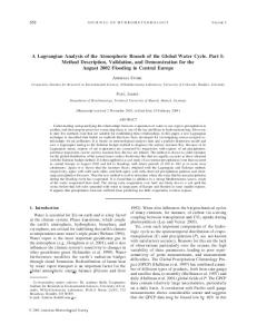
correlations among cues are present, the stability of the estimates can be reduced. In order to compensate for the resulting instability, the number of cases judged must be increased . Complex interactions among these three factors determine their effects. Examples in Figure 1 show how various levels o f - each of these factors affect the standard error of the regression coefficient. This standard error is a statistical estimate of the instability of the judgment model for a particular judge over repeated judgments of the same set of cases. The standard error is only an estimate, subject to

Judgment analysis

T. R . Stewart

48

49

error itself, and is therefore only a rough indication of stability. Its computation is based on conventional assumptions tl,*r!d i n linear multiple regression analysls wtiictl a r c presented in standard texts such as Draper and Smith (1981) and Pedhazur (1982). If the standard error is high, the analysis will be unreliable. .6

m.2

r,* = .o

R

R

=.?

If a maximum acceptable standard error is chosen, it is possible to derive some rough guidelines f o r the number of cases required. For example, a reasonable maximum value for the standard error might be .lo. If the standard error is as high as .lo, then a statistically significant beta weight (a = . 0 5 ) is .20 .25. depending on the number of cases and number of cues. Table 1 presents the approximate minimum number of cases required to achieve a standard error as low as .10 un-

= .7

fi7.6

4

\\

Sf,

-

.2

.c 0

I00

N

-

.6

nor€:

m.2

f,, =

r,, = .o

of weights in judgment analysis could be computed from fewer trials than would be suggested by statistical theory. If Cook's results are substantiated, the usual statistical pro-

/he correlolion be1 ween cue

.4

der various conditions. These minima are presented for illustration only. The actual number of cases needed will depend on the nature of a particular task and, in particular, on the degree of statistical stability desired. Cook (1976) suggests that standard statistical assumptions may not apply to J A . Cook found that stable estimates

100

N

0

I

ond cue

2

R = I h e m u l l i p l e correlation

-

for t h e j u d g e

cedures f o r estimating the stability of regression weights

ti7 = l h e number o f p r e -

Rz.5

dictors

R=7 N

:

/ h e number

at

Cases

SE,= the sfandord error

R= .9

Of

e s t l m a / e for t h e standord p a r t i a l regression

.ol

c o e f f i c i e n t f o r cue I '

0

N

I00

Figure 1. Standard error of the regression coefficient as related to tho number of predictors ( I I I ) , the intercorrelation between cue 1 and cue 2 ( r ) and the multiple correlation between cues ah2 predictors ( R ) .

1

will be too conservative for JA. It may turn out that an investigator using standard procedures would include more cases than necessary in a judgment task. Cook's results have yet to be replicated and extended: but they suggest that present procedures may yield adequate precision. In constructing a judgment task, it is better to err in the direction of including too many cases than too few. The cost of including too few cases is unstable, misleading results. '1,110 cost of including too many cases is that the judges may become tired - a problem that can be overcome by administering the task in more than one sitting.

T.

CL,

R.

Stewart

Judgment analysis

Table 1. Approximate minimum number of cases required to achieve a standard error of the beta weight f o r cue 1 as low a s .10 under various levels of cue intercorrelation, r , and number of cues, m. R , tlic iiiultiple correlition between cues arid judgineiits, is assumed to be . 9 0 . ' A l l intercorrelations other r 1 2 are assumed to be zero.

8

lo

30

30

30

35

40

45

110

115

Exercise of judgment During this step the investigator asks the judges to consider each case and to rate it on the judgment scale. Methods for preparing and presenting cases and for recording judgments must also be considered. Both paper and pencil and interactive computing methods have been used. The cue values must be displayed clearly and unambiguof course, the investigator is interested in ously (~~iiless, studying the effects of ambiguity). If there is a possibility that two judges could disagree about the value of a cue for a given case, the analysis could be misleading because differeiices between judges might reflect differences in cue

- - - - -- - - - -

interpretation rather than differences in cue utilization. Bar graphs have often been used for case presentation because ( a ) tliey are easily and clearly read, (b) ttiey provide a pictorial display of cue information, and (c) they show clearly where the value of each cue is relative to its total ~,i~ige and relative to the values of the other cues. Examples of methods for case presentation will be found

In two recent studies, the author has used the following design: a 50 cases followed by a b

51

throughout this volume.

break (5 minutes to one week), followed by

C 25 crossvalidation cases, followed by d) 25 repeated cases from the first 50.

D a t a analysis: Linear multiple regression

There were six cues in both studies. The cue intercorThis section describes the analysis of judgments b y multiple regress I o n analysis to produce a statistical model of judgment policy. The model describes judgment policy in terms of weights, function forms, and organizing principle. W h s n more than one judge makes judgments about a set of cases, there are two possible ways to analyze the data. The

relations were low in one study and moderate in the other. Multiple correlations were typical of those obtained i n judgment studies. Judges required less than 2 hours to complete all judgments. The repeated cases included all the even numbered cases from the derivation sample and were presented in a random order. F o r typical numbers of cues (4-10), moderate cue intercorrelations, and typical multiple correlatioiis, this design provides an adequate sample size for statistical analysis while not taxing the judges' patience. It also permits crossvalidation of the judgment model and assessment of the judge's reliability.

1

data can be averaged over judges to obtain a mean judgment for eacli case and then those mean judgments can be analyzed. T h i s me tliod is called "nornothetic". Alternatively, j udginents can be analyzed separately for each judge. This method is called "idiographic". Nomothetic and idiographic methods generally yield different results.

T. R . Stewart

Judgment analysis

Judgment analysis is always idiographic, that is, judgments are never pooled or averaged across judges before being analyzed. For a discussion of this important research issue, see Hammond, McClelland and Mumpower (1980, pp. 117-

consistent, a low value does not necessarily indicate that the judge is inconsistent. It could be caused by a poor fit of the 1 Illear model to the judge's policy even though the judge is applying that policy consistently. Without an inde-

52

119 )

.

53

pendent measure of the reliability of the judge, it is not possible to determine with certainty whether a low R is due to inconsistency or to a poor fit of the regression model to

Multiple regression analysis develops an equation to express the relation between one variable, called the dependent variable, and several others, called the predictors or the independent variables. In toe case of judgment analysis, the dependent variable is the judgment and the independent variables are the cues. Regression analysis is used to determine weights for the cues that will best reproduce the judgments. The analytic techniques described in this chapter are based on multiple regression analysis and a basic famil-

a consistently applied policy. The regression equation can be used to predict judgments, but is limited as an aid to understanding judgments because the weights do not necessarily reflect the relative importance of the cues to the judge. Weights are strongly influenced by t h e units in which the cues are measured and therefore one weight cannot be compared to another if the

iarity with such analysis is assumed. Multiple regression analysis produces an equation which can be used to predict the judge's rating of any case. The -regression equation is:

cues are measured in different units. For example, if one cue was expressed as an percentage and another in years (e.g., cluration of a contract), then the relative magnitudes of the regression weights would reflect differences in units more than differences in importance.

Y'

-

a + blXl + b2X2 +

...

+ bkXk

Alternative measures of relative importance

where a is defined as the intercept constant and k is the The concept of relative importance plays a central role in

number of cues. The values of X i in this equation are the cue values for a given case. The regression analysis yields

judgment analysis. Under certain conditions, judgment analysis provides a precise measure of the relative importance of

values for the weights ( b . ) and the intercept constant (a) so that the predicted judgments (Y') will be as close as possible (where "close" is defined in the least squares sense) to the actual judgments (Y) which were made for every

the cues to the judge. Unfortunately, the conditions under which jiitlqinent analysis can provide precise and unambiguous measures of the relative importance of cues do not always

case. The regression equation can be used to predict an individual's judgments. The accuracy of such predictions depends on how well the regression model fits the judge's policy and on how consistently the judge applies that policy. The multiple correlation (R) measures how well the regression model fits a set of judgments. R is related to the consistency or reliability of a judge, but it is an imperfect measure of consistency. While a high value of R indicates that the model fits well and that the judge is highly

occur. It is important, therefore, to understand the difficulties of measuring relative importance and the limitations of multiple regression analysis in this regard. Measures of relative importance derived from multiple regression analysis are unambiguous only when the cues are not interrelated in any way, i.e., wlien the cue intercorrelations are zero. When this is not the case, different measures of relative importance yield different values, and it is not possible to argue that any measure is the correct one, or indeed, to be certain that there is a single correct

'.

54

Judgment analysis

T.. R : Stewart

measure. Darlington ( 1 9 6 8 ) has,discussed in detail various measures of relative importance. In this section, the advantages and limitations of the three most common approaches to measuring relative importance - cue-judgment correlations, standardized regression coefficients, and are discussed. In a later Hoffman's relative weights section a fourth method is introduced that has some advantages when the analysis is not limited to linear functions of the cues. Cue-judgment correlations. These correlations have been called "cue dependencies" in judgment research. They indicate the strength of the linear relation between each cue and the judgment and are simple bivariate correlations that do not take into account variation in any of the other cues. When cues are uncorrelated, cue dependencies reflect the relative importance of cues, because they represent the amount of variation in judgment that can be explained by variation in each cue. When cues are intercorrelated, however, cue

-

dependency may be either inflated or depressed. For example, suppose that an admissions officer ignored the College Entrance Exam scores and relied totally on high school grades for admissions decisions. Since the exam score is related to

55

ment without changing the correlations among them. A s a result, the relative magnitudes of the beta weights for different C ' I I C S can be directly compared. A s measures of relative importance the Oils are supe-

hi's

rior to the because differences due to units of measuremeiit are removed. Beta weights are also generally superior to cue dependencies, because the procedure for deriving beta weights controls for variation in other variables. The beta weight for a cue provides an estimate of its effect on judgiiic%ilt with the other cues held constant. In other words, the b e t a weight estimates the direct impact of a cue on the set of judgments. Itoffman's relative weights. This might be considered a hybrid weighting procedure because it measures weights by computing the product of the cue dependency and the beta weight. That product i s divided by the squared multiple correlation coefficient ( R 2 ) . lhe

formula f o r relative weights is

riBi RWi =

-----R2

high school grades, the cue dependency for the exam score could be substantial even though it had no impact at all on

where ftWi is the relative weight for cue i, ri is the cue

the judgment. The cue dependencies would be high simply because the exam score is related to grades and grades strongly influence the judgment. In this case the importance of

dependency for cue i, and Bi is the beta weight for cue i. Relative weights computed by this method, which was proposotl by Hoffman in 1 9 6 0 , are influenced both by the overall linear relation between the cue and the judgment and by the statistically estimated direct relation. Darlington (1968) criticized this method for computing relative weights on the grounds that it does not solve the problems caused by

the cue is negligible, while the cue dependency could be substantial. For this reason, cue dependencies should never be used as measures of importance when cues are interrelated. Standard regression coefficients. Standard regression coefficients, often called beta weights (Bi), a r e the weights that would be obtained from a regression analysis involving the cues and judgment expressed in standard score form, that is, adjusted to have a mean of zero and a standard deviation of one. The effect of this adjustment is to remove differences among the cues due to scales of measure-

cue intercorrelations and it provides a measure which has no clear statistical interpretation. Although Hoffman's relative welcjtit method is still being used, beta weights are preferable. A full discussion of the concept of "relative importance" and possible ways of measuring it is beyond the scope of this chapter. The interested reader should consult the ex-

J u d g m e n t analysis

T. R . Stewart

5b

51

cellent paper by Darlington (1968). The reader should also

tions requlred to justify the use of this model: linearity

be aware that the topic is controversial. Authors who have recently commented on this topic include Andcrson ( 1 9 8 2 ) ; Stillwell, Barron and Edwards (1983); Lane, Murphy and Marques (1982) and Surber (1985).

and additivity. L f n c d r f t y . The use of linear regression assumes that the relatlon between each cue and the judgment is linear, that is, the impact of one additional unit of cue value on the judgment does not change at different levels of the cue.

The following points are important: 1. When the cues are not correlated, relative impor-

For example, a linear relation between wage increases in a

2.

tance measured by cue dependencies, beta weights or Hoffman's relative importance measure will yield the same results. When cue intercorrelations are moderate, cue depen-

3.

dencies should not be used as measures of relative importance. Beta weights will generally provide good measures of relative importance. When cues are highly intercorrelated, measures of relative importance become virtually useless, because (a) they are subject to large errors of estimation, and (b) their meaning is unclear because it is impossible to separate the effects of one cue from those of others that covary with it.

Function form

labor contract and the acceptability of the contract would imply that average) difference in acceptability between contracts with 3.0% and 4 . 0 % wage increases would be the same as that between contracts with 6.0% and 7.0% wage increases. If the change In acceptability of a contract due to a 1% increase in wage depends on level of increase, then the relation is not linear.

Additivity. The linear regression model assumes that the organizing principle is additive, that is, the effects of one C I J Pdo riot depend on the levsls of others. The organizing principle is nonadditive if the effect of one cue changes as levels of other cues change. The following statements de:,cribe some judgment policies that are nonadditive: 1. Cue 1 is only considered when Cue 2 is high. 2. If all cue values are high, then the judgment is high, otherwise the judgment is low (conjunctive model ) 3. If any cue is high then the judgment is high,

.

Function form represents the relation between a single cue and the judgment. In a linear analysis, two types of function forms are possible: positive linear and negative linear. Each function form can be indicated by the sign of the

4.

regression coefficient. A positive regression coefficient

otherwise the judgment is low (disjunctive model). lhe weight on Cue 1 increases as the value of Cue 2 increases (multiplicative model).

denotes a positive linear function form and a negative regression coefficient indicates a negative linear function form. Function forms are discussed in more detail below in

5.

connection with nonlinear analysis.

The number of possible nonadditive policies is unlim-

The judgment increases as the amount of discrepancy between Cue 1 and Cue 2 increases (absolute value of difference model).

Assumptioris of l i n e a r , a d d i t i v e r e g r e s s i o n model

ited. Some possible models are discussed in more detail in a later section. If either the additivity or the linearity assumptions

The linear, additive model discussed so far has been and will continue to be a powerful tool in judgment analysis. The investigator should be aware, however, of the assump-

are unreasonable for a particular judgment problem, then the linear model may be misleading. The linear model should be abandoned reluctantly, however, for to do so may introduce

Y

T. R. Stewart

Judgment analysis

complexities into the analysis that outweigh possible gains in accuracy. The linear model has the advantage that it can describe accurately many processes that are not strictly linear (Dawes & Corrigan, 1974). In particular, as long as the relations between the cues and the judgment are monotonically increasing or decreasing, the linear model is likely

The correlation coefficient corrected for inconsistency (G). One might ask, "What would be the relation between the judgments of two judges if each applied his or her regression model with perfect consistency?" A measure of agreement between the judges is needed that is independent of the consistency with which each policy is applied. We can construct such an index in the following way: 1. Apply the policy of each judge to the set of cases to derive a set of "predicted judgments" (Y'). These are the judgments that judges would make if they were to apply their judgment policies with perfect consistency. 2 . Compute the correlation between the predicted judgments for the two judges. This correlation has traditionally been called G. If the judgment policies of two judges are different, i.e., the judges disagree "in principle", then G will be low. If the judgment policies are similar, then G will be high.

58

to do well. The linear model can often describe complex processes in a simple form that can be more easily understood by a judge than a complex mathematical model that might more faithfully represent the process (Dhir & Stewart, 1984). Generally, the goal of JA in the context of Social Judgment Theory is to derive a useful description of the judgment process and not necessarily to reproduce faithfully all the properties of the process itself (Hammond et al., 1975). Data analysis: Comparing two systems In many JA applications it is desirable to compare several judges or to analyze the relation between one or more judges and a criterion. When judgment analyses have been conducted f o r all judges and criterion ("judgment analysis" for a criterion is simply the analysis of task data by means of multiple regression techniques), the relations among pairs of judges or between individual judges and the criterion can be analyzed. Three indices of the relation between two systems will be described briefly here. The correlation coefficient (ra). The correlation between a set of judgments made by two judges over the same cases reflects the overall agreement between them. If ra is high, then they will agree closely on most judgments. If it is low, they can be expected to disagree on most judgments. The overall index of agreement can be low either because (a) the judges may agree in principle (i-e., have the same policy) but apply it inconsistently (i.e., have low multiple correlations), or because (b) they may be consistently applying judgment policies which are dissimilar. Fortunately, there are methods of discovering why agreement is low.

5'

Provided that the correct model is used, the consistency with which a judgment policy is applied can be measured by R, the multiple correlation coefficient. Since G and R are independent, they provide separate measures of the relation between two judges' policies and their consistency. The correlation between residuals (C). For each judge, "residuals" are obtained by subtracting predicted judgments based on the judgment policy from actual judgments. These residuals are the differences between the ratings that the judge would have given the cue profiles if applying the judgment policy with perfect consistency and the ratings actually given. The correlation between two judges' residuals is called "C". C reflects the relation between those parts of two individuals' judgments not accounted f o r by linear regression models of their judgment policies. In order to interpret C, it is necessary to further understand the residual component of judgment. Variation in judgment has three components: (a) the part explained or described by the regression model of the judgment policy, i.e., the predicted variation: (b) a systematic part consistently related to the cues but not to the regression model,

60

T. R. Stewart

i.e., systematic variation not predicted by the model, and (c) an unsystematic, random part due to unreliability of judgments. If the judgments of two judges are divided in this way, the correlation between the two predicted parts is G, as explained above. The two remaining parts, systematic

and unsystematic, constitute the residual. Unsystematic variation should not correlate with anything, except by chance. Systematic variation may be related to systematic variation in the judgments of another. If C for two judges is high, it must be because (a) a substantial proportion of the residual for the judges is systematic and (b) the systematic variation in the two sets of judges is closely related. If C is low, it may be because the systematic components for the two judges are unrelated, unimportant, or both. In order to separate these two possibilities, the proportion of variation due to random components would have to be estimated through the use of repeated profiles as described above. In general, high values of C are not desirable and are, in fact, disturbing. A high value of C indicates that the analysis was potentially inadequate f o r both judges, because a substantial part of the residuals from the judgment policy is due to systematic variation in the cues. High C values therefore indicate that the analysis does not account for all the consistent variation in a judge. A s a result, the judgment policy may misrepresent the importance of the cues to the judge, as well as the functional relations and organizing principle. While high values of C indicate the presence of effects not described by the judgment policies, the converse is not true. That is, low values of C do not indicate the absence of systematic components in the residuals. Low C values merely indicate the absence of shared systematic variation in the residuals. It would still be possible for both judges to have large systematic components in the residuals which were unique to each. For example, if one is using nonlinear policy A and another is using nonlinear policy B, the C coefficient computed f o r the two may be quite low, even though the linear regression provides a poor model of each judge.

Judgment analysis

61

Therefore, although high C values often indicate possible inadequacies of the linear model, low C values do not guarantee that the linear model is adequate. In summary, the three measures, ra, G, and C tell us different things about the relation between two sets of judgments (or the relation between a person's judgments and a criterion). 1. r is an index of overall agreement. a 2 . G measures the correspondence between the models of the judgment policies of the two judges. If G is high, the models correspond. If G is low, the models differ. G is not affected by the consistency with which the models are applied. 3 . C measures the correspondence between the residuals from the regression model for the two judges. A high value of C indicates that the residuals contain a systematic component and that those systematic components are shared by the two judges. A low C value is ambiguous because we cannot be sure why it is low. It could be low because the residuals f o r both judges are random and unsystematic (error) variation or because the residuals of one or both judges contain systematic nonlinear components which are unrelated. For an advanced technique of judgment analysis that can be used to refine the C measure, see Stewart (1976). Relation between G, R, ra, and C - the Lens Model Equation The measures described above are related to one another in a particular way. The relation is described by the lens model equation, which was developed by Hursch, Hammond and Hursch (1964) and modified by Castellan (1973), Cooksey and Frebody (1985), Dudycha and Naylor (1966), Rozeboom (1972), Stewart (19761, and Tucker (1964). The form of the equation developed by Tucker (1964) is the best known:

Judgment analysis

T. R. Stewart

62

where r a' G and C are as described above and R1 and R2 are the multiple correlations for the first and second judge. The lens model equation analyzes agreement (or achievement, if judgments are being compared to correct answers) into its components. The first term on the right hand side of the lens model equation is the linear component of agreement, that is, it measures the amount of agreement due to the linear component of judgment. The second term is the nonlinear component of agreement, indicating the agreement due to the component of judgment not captured by the linear model. In most judgment studies, the nonlinear component of agreement is so small that it is negligible, and the linear component is sufficient to explain the reasons for agreement or disagreement. As suggested above, however, the nonlinear component is useful because, if it is large, it indicates that the linear regression model does not capture all of the consistent variation in judgment.

Data analysis: Nonlinear and nonadditive models Although a linear model has been useful in many judgment analysis studies, the investigator should check its ade2 quacy. Such indications include a low R , nonlinear scatterplots of cues vs. judgments, significant lack of fit, and high correlations ( C ' s ) among the residuals. If any of these conditions exist, it is desirable to investigate nonlinear models. It is useful to distinguish between additive and nonadditive nonlinear models. An additive nonlinear model is of the form: Y

=

a + b1f1(X1) + b2f2(X2) +

...

+ bkfk(Xk)

where f.(X.) is some nonlinear function of the cue Xi. In 1

1

these models, the effects of the cues are additive, but the

63

relation between each cue and the judgment is some nonlinear function of the cue (e.g., exponential, quadratic, etc.). If the effects of the cues are combined by some process other than addition, the model is nonadditive. For example, Einhorn (1970) describes procedures for analyzing conjunctive and disjunctive noncompensatory models. (A noncompensatory model is one in which the effects of one cue cannot be overcome or compensated for by another cue.) An additive model is inherently compensatory because the effect of a unit's change in one cue can be balanced by compensatory changes in the others. Nonadditive models will be discussed below.

Additive nonlinear models An additive nonlinear model that has been found useful in JA is the polynomial model formed by adding squared terms to the original regression equation:

Y

=

a + bllXl + b12X 2

+ b21X2

+

b22X 2

..+ bklXk

+

bk2x2 k

where bil is the regression coefficient for the value of cue i and bi2 is the regression coefficient for the square of the value of cue i. This model is additive because the contribution of any cue is independent of the values of the other cues. It is nonlinear because the relation between the cues and the judgment are not all linear. Another term that has been applied to this type of model is "curvilinear". An equation such as the one above can be fitted to a set of judgments by generating new predictors that are added to the original predictors in the regression analysis. The new predictors consist of the squares of the values of the cues suspected to be nonlinear. (For computational reasons, it is better to use the squares of the deviations of the cue values from their means, but the results will be the same.) A variety of function forms useful in judgment analysis can be reproduced by equations involving a cue and its square (Figure 2 ) .

04

J u d g m e n t analysis

T. R . Stewart //XI = 2 x

+ ox’

Separation of weight and function form For additive models, it is useful to describe judgment policy in terms of weight and function form. In the raw form of the regression equation, the coefficients contain sufficient information to determine both weights and function forms, but the two forms are confounded. The following procedure is used to separate weight and function form information: 1. Isolate the two terms in the regression equation that relate to a particular cue. 2 . Define the function form of each cue as the sum of

f f X I =4 . 0 O X - . 2 0 X ~

f ( X l = OX-.2OX’+20

the two terms relating to it. 3. Rescale the function forms so that all have comparable variability. They could be standardized to have a mean of 0.0 and a standard deviation of 1.0 in the sample of cas e s . An alternative procedure would be to rescale them so that all would have the same minimum and maximum values over

“I

= 0x-.0x=

ffw= -ax +.Oxp+20

the range of the cue. The second procedure, called the ”range method” is to be preferred if the natural cue ranges are known because it frees the weights from the influences of the sample cue distributions which may, by chance, differ from the population distributions. The purpose of rescaling i s to remove the influence of relative weights on the function forms. The rescaled functions may be considered pure or unweighted function forms because they are free from the influence of the relative weights of the cues. 4 . Compute regression coefficients for the rescaled function forms by using them as predictors in the regression equations. The regression coefficients will indicate their relative weights. Note that this procedure provides a single weight for each cue (rather than one weight for the cue and another f o r its square) and that the weight reflects the combined influence of the cue and its square. Note also that the resulting regression equation amounts to a linear transformation of the original equation and, therefore, does not change its explanatory or predictive power. If the rescaling

F i g u r e 2. Examples of function forms that have been found useful in JA.

66

T. R. Stewart

is properly done, the multiple correlation based on the rescaled cues will be the same as the multiple correlation obtained before rescaling. The procedure merely produces an equation algebraically equivalent to the original equation but more useful for understanding judgment policy, because weight and function forms are separated and clarified. Nonadditive m o d e l s Nonadditive policies possess one or more of the following properties: 1. The impact of one cue on the overall judgment de pends on the levels of one or more other cues. 2. The judgment depends on the pattern of relations among cues, or the configuration of cue levels, rather than on the separate values of the cues. Such nonadditive models are often called "configural" models in judgment research. 3. The principle for combining the cues into a judgment depends upon the levels of one or more cues. Conjunctive and disjunctive models are two types of nonadditive model. In the conjunctive model the minimum judgment is given unless all cues reach a particular level (or cutoff value). For example, a graduate admissions policy that excludes all candidates with grade point average below 3.0 or a Graduate Record Exam score below 500 would be a conjunctive noncompensatory policy. It is noncompensatory because an increase in GRE cannot compensate for a GPA below 3.0, and it is conjunctive because cutoffs on both criteria must be satisfied before the candidate can be admitted. A disjunctive policy is one in which a cutoff on any one cue must be satisfied. An admissions policy would be disjunctive if applicants possessing either a 3.0 GPA or a 500 GRE score were admitted. This policy is noncompensatory because if either cutoff is satisfied, then the other cue, no matter how low its value, will not affect the decision. Nonadditive models may be attractive to the judgment analyst for several reasons. First, when people discuss the basis for their judgments, they often use language that

Judgment a n a l y s i s

67

implies a noncompensatory, nonadditive policy. Second, the richness and variety of nonadditive models would seem to be required to describe the richness and variety of judgment processes. Third, when professionals teach professional judgment (e.g., in medicine, clinical psychology, law) they teach nonadditive policies. They often teach the aspiring professional to recognize patterns, not to weigh and add cues. In spite of their strong appeal, experienced judgment analysts regard nonadditive models with suspicion and have not used them extensively. Additive models explain most of the systematic variance in many types of judgments. They are adequate for most applications, and the descriptions of judgment provided by additive models are easily understood. Furthermore, the procedures for fitting additive models are well developed and widely available. Although procedures are available for fitting certain classes of nonadditive models (Anderson, 1982; Einhorn, '1970), the search f o r a nonadditive model can easily become a fishing expedition if the investigator succumbs to the temptation to try many models in the hope of discovering the best. A discussion of methods for fitting nonadditive models is beyond the scope of this chapter. Judgment researchers recognize that many different models will frequently provide equally high predictability of an individual's judgments (Goldberg, 1971; Dawes & Corrigan, 1974; Lovie & Lovie, 1986). In fact, a cue profile that sharply differentiates the predictability of different models is something of a rarity. This is a problem if one is interested in how a judge actually organizes information into a judgment. If one is interested in obtaining descriptions of judgment policy that can facilitate understanding, learning or conflict resolution, however, the availability of a range of equivalent models allows the investigator to select the most useful model. This will typically be the simplest model that accounts for the variance in judgment (see Chapter 3 for further discussion).

68

T. R. Stewart

Judgment analysis

Presentation of results

functional relation with the judgment even though they may have different weights. Unweighted function forms separate form of the functional relationship from cue weight. A potential disadvantage of unweighted function forms is that when a cue has a small but nonzero weight, the form of its relation with the judgment may have little meaning. The relation may be slightly nonlinear due to spurious statistical effects in the sample of cases judged. The weighted function form for such a cue appears as a more or less flat line with a slight curve. When this form is rescaled to have the same range as the other cues, the curvilinearity is exaggerated and the resulting unweighted function form may make no sense at all. Consequently, the investigator is left to explain away a function form that is probably spurious. The problem of exaggerating meaningless function forms may be reduced by the use of stepwise regression for the analysis of judgments (Pedhazur, 1982; Draper & Smith, 1981). The stepwise procedure eliminates cues from the analysis when they do not have substantial weight. This effectively gives cues a weight of zero when their weight is not substantial enough to contribute significantly to the analysis. The function form for a cue with no weight is a horizontal straight line.

In many applications of JA it is desirable to describe the results to the judges in a way that helps them understand their own judgment policies, facilitates interpersonal learning or task learning, or aids in conflict management. The usual method for displaying results of judgment analysis is to generate graphs showing the weight and function form for each cue. Displays of weights and function forms can be found in Chapter 5. Although the display of results is generally straightforward, two alternatives regarding the scaling of weights and function forms before presention to the judges must be considered. Raw weights vs. relative weights. The raw standardized regression coefficients (beta weights) and the weights obtained by any rescaling method will be influenced, to a degree, by the consistency with which the judge applies his or her policy and the variability of the judgments. To remove these effects, relative weights may be computed by adjusting the raw weights so that they sum to 1.0 or 100. Relative weights are more easily interpretable, because it is easy to assess the proportional influence of each cue. For most applications, relative weights will be preferred to raw weights. Weighted vs. unweighted function forms. The function form plots presented to the judge may be scaled so that they all have equal ranges (unweighted), or they may be plotted in their original form (weighted). Weighted function forms contain information about the cue weight as well as the form of the relation between the cue and the judgment. Weighted function forms for less important cues are less steep and have a smaller range, than the forms for the more important cues. Unweighted function forms have the advantage of being pure descriptions of the functional relationship without confounding information about weight. Two cues with identical unweighted function forms can be said to have the same

I

I

69

Reporting research results The reporting of results of JA studies in the research literature has not been standardized. Often, critical elements of the research design, such as the cue intercorrelations, are not reported. This makes it difficult to evaluate and interpret the results of a study. The following items should be included in a research report: 1. Descriptions of the judges and how they were selected. 2 . Descriptions of the cues and how they were chosen. 3. Definition of the judgment and the response scale. 4. Distributions of the cue values and how they were generated.

T. R. Stewart

70

Judgment analysis

5. Intercorrelations among the cues. 6. Reliabilities of the judges, computed by correlating their judgments over repeated cases.

References

7. Multiple correlations for linear models and for any

Anderson, N. H. (1902). Methods of information integration

nonlinear models investigated. 8. Standard errors of the regression coefficients. 9. Relative weights and the method used to calculate them.

theory. New York: Academic Press. Castellan, N. J., Jr. (1973). Comments on the "lens model"

10. Function forms, if nonlinear function forms were used.

Conclusion

71

equation and the analysis of multiple-cue judgment tasks. Psychometrika, 38, 87-100. Chapman, L. J. & Chapman, J. P. (1969). Illusory correlation as an obstacle to the use of valid psychodiagnosL I C signs. Journal of Abnormal Psychology, 7 4 , 271-280. Cook, R. L. (1976). A study of interactive judgment analysls and the representation of weights in judgment policies.

This chapter has discussed the steps involved in carrying out a JA study and has described the analytic procedures used. Applications of JA require a series of design decisio n s that are guided by principles of Social Judgment Theory, statistical data analysis, and psychometrics. The analysis of data can be accomplished with standard computer statistical packages1 J A is not.the only method for developing algebraic models of the judgment process. Multiattribute

.

utility theory (e.g., Edwards

&

Newman, 1982), functional

Unpublished doctoral dissertation, University of Colorado. Cooksey, R. W. ti Freebody, P. (1985). Generalized multivarlote lens model analysis f o r complex human i n f e r e n c e tasks. Organizational Behavior and Human Decision Processes, 35, 46-72. Darliriqton, R. 8. ( 1968). Multiple regression in psychological research and practice. Psychological Bulletin, 69, 161-182. Dawes, R. M. & Corrigan, B. (1974). Linear models in deci-

measurement (Anderson, 1902), conjoint measurement (Green & Rao, 1971; Wigton et al., 1986) and the analytic hierarchy process (Saaty, 1980) all produce quantitative judgment

sion making. Psychological Bulletin, 81, 95-106. Dhir, K. S. & Stewart, T. R. (1984). Models and management:

models. J A differs from these approaches in one important respect: J A is the only method that is based on the theoretical premises of SJT and on Brunswik's lens model. Because

Bridging the gap. Proceedings of the National Meeting of the American Institute f o r Decision Sciences. D r a p e r , N. & Smith, H. (1981). Applied regression analysis,

of this theoretical foundation, JA emphasizes the representative design of judgment tasks, and is based on a statisti-

(2nd Ed.) New York: Wiley. Dudycha, L. W. ti Naylor, J. C. (1966). Characteristrcs of tile human inference process in complex choice behavior situations. Organizational Behavior and Human Performance, 1 , 110-128. Edward,,, W. & Newman, J. R. (1982). Multiattribute evalua-

-

cal method multiple regression analysis enough to handle representative designs.

-

that is flexible

Footnote 1. An interactive JA program for personal computers is available from Executive Decision Services, P.O. Box 9102, Albany, N.Y. 12209.

tion. Beverly Hills: Sage Publications. Einhorn, H . J. (1970). The use of nonlinear, noncompensatory models in decision making. Psychological Bulletin, 73, 221-230.

T. R. Stewart

Judgment analysis

Goldberg, L. R. (1971). Five models of clinical judgment: An empirical comparison between linear and nonlinear representations of the human inference process. Organizational Behavior and Human Performance, 6, 458-479. Green, P. E. & Rao, V. R. (1971). Conjoint measurement for quantifying judgmental data. Journal of Marketing Research, 8, 355-363. Bammond, K. R. & Adelman, L. (1976). Science, values, and human judgment. Science, 194, 389-396. Hammond, K. R., Anderson, B. F., Sutherland, J. & Marvin, B. (1984). Improving scientists' judgments of risk. Risk Analysis, 4 , 69-78. Hammond, K. R., McClelland, G. H. & Mumpower, J. (1980).

Lovie, A. D. & Lovie, P. (1986). The flat maximum effect and linear scoring models for prediction. Journal of Forecasting, 5 , 159-168. Miesling, P. & Dandrige, T. C. (1986). Judgment policies used in assessing enterprise-zone economic success criteria. Decision Sciences, 17, 50-64. Pedhazur, E. J. (1982). Multiple regression in behavioral research (2nd Ed.) New York: Holt, Rinehart & Winston. Roose, J. E. (1974). Judgmental prediction as a selection device in the Travelers Insurance Company. Unpublished Master's Thesis: Bowling Green State University. Rozeboom, W. W. (1972). Comments on Professor Hammond's paper on inductive knowing. In J. Royce & W. Rozeboom (Eds.), The Psychology of knowing. London: Gordon & Breach. Saaty, T. L. (1980). The analytic hierarchy process. New York: McGraw-Hill. Stewart, T. R. (1976). Components of correlations and extensions of the lens model equation. Psychometrika, 41, 101-120. Stewart, T. R. & Ely, D. W. (1984). Range sensitivity: A

72

Human judgment and decision making: Theories, methods, and procedures. New York: Praeger. Hammond, K. R. & Stewart, T. R. (1974). The interaction between design and discovery in the study of human judgment. (Center f o r Research on Judgment and Policy Report No. 152) University of Colorado at Boulder, Institute of Cognitive Science. Hammond, K. R., Stewart, T. R . , Brehmer, B. & Steinmann, D. 0. (1975). Social judgment theory. In M. Kaplan & S. Schwartz (Eds.), Human judgment and decision making. New York: Academic Press. Hoffman, P. J. (1960). Paramorphic representation of clinical judgment. Psychological Bulletin, 5 7 , 116-131. Hursch, C. J., Hammond, K. R. & Hursch, J. L. (1964). Some methodological considerations in multiple-cue probability studies. Psychological Review, 71, 42-60. Kirwan, J. R., Chaput de Saintonge, D. M., Joyce, C. R. B. & Currey, H. L. F. (1984). Clinical judgment in rheumatoid arthritis: 111. British rheumatologists' judgments of 'change in response to therapy'. Annals of the Rheumatic Diseases, 43, 686-694. Lane, D. M., Murphy, K. R. & Marques, T. E. (1982). Measuring the importance of cues in policy capturing. Organizational Behavior and Human Performance, 30, 231-240.

73

necessary condition and a test for the validity of weights. (Center f o r Research on Judgment and Policy Report No. 270). University of Colorado. Stillwell, W. G., Barron, F. H. & Edwards, W. (1983). Evaluating credit applications: A validation of multiattribute utility weight elicitation techniques. Organizational Behavior and Human Performance, 32, 87-108. Surber, C. F. (1985). Measuring the relative importance of information in judgment: Individual differences in weighting ability and effort. Organizational Behavior and Human Decision Processes, 35, 156-178. Tucker, L. R. (1964). A suggested alternative formulation in the developments by Hursch, Hammond, & Hursch, and by Hammond, Hursch, & Todd. Psychological Review, 71, 528530.

T. R . Stewart

74

Wigton, R. S., Hoellerich, V. L. & Patil, K. D. (1986). H o w physicians use clinical information i n diagnosing p u l molia1-y

embolism:

An

application of conjoillt: analysis.

Medical Recision Making, 6,

2-11.