STATISTICS IN MEDICINE Statist. Med. 2001; 20:2965–2976 (DOI: 10.1002/sim.912)

Understanding neural networks using regression trees: an application to multiple myeloma survival data David Faraggi1;∗ , Michael LeBlanc2 and John Crowley2 1 Department

2 Fred

of Statistics; University of Haifa; Haifa; 31905; Israel Hutchinson Cancer Research Center; Seattle; Washington; U.S.A.

SUMMARY Neural networks are becoming very popular tools for analysing data. It is however quite di8cult to understand the neural network output in terms of the original covariates or input variables. In this paper we provide, using readily available software, an easy way of understanding the output of the neural network using regression trees. We focus on the problem in the context of censored survival data for patients with multiple myeloma, where identifying groups of patients with di;erent prognosis is an important aspect of clinical studies. The use of regression trees to help understand neural networks can be easily applied to uncensored situations. Copyright ? 2001 John Wiley & Sons, Ltd.

1. INTRODUCTION The Cox proportional hazard model [1] is the most widely used model that relates covariates to censored survival data. In recent years di;erent models have been proposed as possible alternatives. These models range from the fully parametric Weibull survival model [2] to the accelerated failure time model [3], to much more computer intensive methods. These models include regression trees [4], splines [5; 6] and neural networks [7], to name a few. One of the main di;erences between these computer intensive models is that both the neural network and spline models Bt a smooth function of the covariates to the hazard function. The regression tree, on the other hand, splits the covariates to form interpretale risk groups for survival, and yields a piecewise constant regression surface model. Neural networks are known to be very powerful tools for modelling an arbitrary non-linear relationship between covariates and response. These models have been extensively used in many research areas ranging from marketing [8] to brain research [9]. For most applications the best-Btting models are smooth functions of the predictor variables. However, in many situations, in addition to Bnding a good smooth approximation that relates the covariates to the response, it is desirable to split the observations into mutually exclusive groups. In particular, in clinical trials, forming easily interpretable risk groups for patients is a desirable feature of any statistical model and analysis. When a model such as the neural network is ∗ Correspondence

to: David Faraggi, Department of Statistics, University of Haifa, Haifa 31905, Israel

Copyright ? 2001 John Wiley & Sons, Ltd.

Received December 1999 Accepted October 2000

2966

D. FARAGGI, M. LEBLANC AND J. CROWLEY

Btted to survival data, it is not clear how one should proceed with forming subgroups that are intuitive. The aim of this paper is to propose such a method. Our proposed method is based on growing a regression tree on the output of the neural network. The use of neural networks in conjunction with regression trees gives the user a way to implement the power of the neural network model to obtain a good continuous approximation of the hazard function, and in addition to construct interpretable risk groups that are a natural outcome of the regression tree. We will illustrate our proposed method on data from patients with multiple myeloma. We show that in terms of prediction on a real validation sample, the neural network achieved the best results among the models presented. More importantly, we show that when a neural network is used in conjunction with a regression tree, the tree provides a useful tool for understanding which variables or combinations of variables yield an association with larger or smaller predicted values. The rest of the paper is organized as follows. In Section 2 we present survival data on patients with multiple myeloma and a commonly used staging system. In Section 3 we present both the neural network and the regression tree and explain how to apply the regression tree to the output of the neural network. In Section 3 we apply the above to the myeloma data to form risk groups, and compare these results to those obtained from the commonly used Cox regression model. We conclude with some Bnal comments. 2. SURVIVAL OF PATIENTS WITH MULTIPLE MYELOMA – AN EXAMPLE Multiple myeloma is a malignancy of the plasma cells of the bone marrow. With standard treatment the median survival for patients is from 30–36 months. In recent years two successive trials on patients with multiple myeloma were carried out by the same muli-centre group, the Southwest Oncology Group [10; 11]. Both tested variations on combined chemo-hormonal therapy. SWOG study 8229 (started in 1982, n = 532) compared two alternative schedules of administration of the same set of chemotherapeutic agents and found no di;erence in survival [10]. SWOG study 8624 (started in 1986, n = 479) compared one of the arms of 8229 with two other regimens and found some advantage to higher doses of steroids [11]. The two survival curves, collapsed over treatment arms, are shown in Figure 1(a). We will use the data from 8229 for model building and the data from 8624 for validation of the results. A commonly used staging system was developed by Durie and Salmon [12]. It takes into account the number of tumour cells (I, II or III) and classiBcation of kidney impairment (A or B). Figure 1(b) shows the data of SWOG 8624 collapsed into three groups (I–II, IIIA and IIIB). To illustrate the methodology proposed in this paper, we examine these data along with Bve covariates of interest. The covariates are: age (in years); serum 2 microglubulin (indicates both tumour volume and kidney failure); calcium (indicates bone loss); albumin (indicates nutritional status), and creatinine (indicates kidney failure). 3. METHODS FOR CLASSIFICATION AND PREDICTION 3.1. Neural network The neural network [13] non-linear function deBnes the relation between the covariates and the response. The model includes nodes that are organized in layers. The Brst layer is called Copyright ? 2001 John Wiley & Sons, Ltd.

Statist. Med. 2001; 20:2965–2976

UNDERSTANDING NEURAL NETWORKS USING REGRESSION TREES

2967

Figure 1. (a) Survival for SWOG 8229 and 8624. (b) SWOG 8624 survival by Durie–Salmon.

the input layer (covariates) and the last one is called the output layer (response). The layers in between are called hidden layers. In this paper we will restrict ourselves to a single hidden layer neural network with a single output (response) as is illustrated in Figure 2. Each node in the input layer is connected to all but the Brst node in the hidden layer and each node in the hidden layer is connected to the node in the output layer. Copyright ? 2001 John Wiley & Sons, Ltd.

Statist. Med. 2001; 20:2965–2976

2968

D. FARAGGI, M. LEBLANC AND J. CROWLEY

Figure 2. The structure of a single hidden layer feed-forward neural network model.

Consider the ith patient with P covariates, where xi = (xi0 = 1; xi1 ; : : : ; xiP ) is a 1 × (P + 1) input vector (i = 1; : : : ; n). !h = (!0h ; : : : ; !Ph )
is a (P +1) × 1 vector of parameters connecting the inputs to the hidden node h (h = 1; : : : ; H
). The input to the h
node in the hidden layer for the ith patient is the weighted sum xi !h = Pp=0 xp !ph = !0h + Pp=1 xp !ph . The output from any node in the hidden layer is its input transformed by a squashing function, such as the logistic function, f() = {1+exp(−)}−1 . Hence the output of the ith patient from the h node in the hidden layer is f(xi !h ). Finally, the output of the network is a linear combination of the outputs from the nodes in the hidden layer with parameters  = (0 ; 1 ; : : : ; H ). Consequently the output from a single hidden layer neural network with H hidden nodes for a given patient with input vector xi = (1; xi1 ; : : : ; xiP ) is g(xi ; ) = 0 +

H


h f(xi !h ) = 0 +

h=1

H


h h=1 1 + exp(−xi !h )

(1)

where  = (!01 ; !11 ; : : : ; !P1 ; !02 ; !12 ; : : : ; !P2 ; : : : ; !0H ; !1H ; : : : ; !PH ; 0 ; 1 ; : : : ; H ) denotes the vector of unknown parameters. The number of parameters in (1) is (P + 1)H + (H + 1). For further discussion on neural network see, for example, Wasserman [14]. The Cox proportional hazards model [1] relates the hazard function at time t to a vector of covariates xi for the ith patient through h(t; xi ) = h0 (t) exp(xi )

(2)

where h0 (t) is the baseline hazard and  = (0 = 0; 1 ; : : : ; P )
. The unknown parameters  are estimated by maximizing the log of the partial likelihood as suggested by Cox [15]

{x(i)  − log exp(xj )} (3) i

where x(i) are the input values of the ith ordered uncensored observation t(i) , and the second summation is over the risk set at t(i) . For further discussion see Miller [16]. To obtain the neural network model for survival data we follow Faraggi and Simon [7] and replace the linear combination of the covariates xi  in (2) with the output of the neural network g(xi ; ) to obtain h(t; xi ) = h0 (t) exp(g(xi ; )) Copyright ? 2001 John Wiley & Sons, Ltd.

(4) Statist. Med. 2001; 20:2965–2976

UNDERSTANDING NEURAL NETWORKS USING REGRESSION TREES

2969

Figure 3. Graphical illustration of the curtailed estimation procedure.

and the function to be maximized becomes

{g(x(i) ; ) − log exp[g(xj ; )]} i

(5)

Note that similarly to the usual proportional hazards model where one does not include the constant term, we here too omit 0 from , so that the total number of parameters in (4) is K = (P + 1)H + H = (P + 2)H . Faraggi and Simon [7] suggested using maximum likelihood estimates (MLEs) for the parameters of the neural network and used the Newton–Raphson method [17] to maximize the log of the partial likelihood in (5). One of the major advantages of the non-linear function, deBned by the neural network, is its Nexibility. With enough parameters, it can approximate, to any degree of accuracy, any well-behaved function [18]. This Nexibility also causes the model to over-Bt the data, that is, the model is Btted too closely to the data and follows also its noise, so that it is poorly generalized to other data sets drawn from the same population [19; 20]. Several methods have been proposed to prevent the model from over-Btting: limiting the number of parameters in the model [21]; penalizing for the size of the parameters [19; 22], and curtailed training [21]. The method of curtailed training assumes that over-Bt occurs at the latter stages of the estimation procedure. During the initial stages of the estimation, for example, the Newton–Raphson iteration procedure [17], the noise in the data does not a;ect the estimates; only during the latter stages of the procedure are the parameter estimates inNuenced by the noise in the data. Consequently there exists a point during the estimation procedure when over-Bt starts. To locate this point we divide the model building data set into two subsets of equal size. On the Brst half (the training set) we estimate the parameters while on the second subset (the stopping set) we evaluate the criteria in (5), with the values of the parameters obtained from the training set. A graphical illustration of the curtailed training procedure is presented in Figure 3. While the log-likelihood values in the training set are always non-decreasing, for the stopping set there is a point where the log-likelihood reaches its maximum and then decreases. At this point we assume that over-Bt starts and we curtail our estimation process Copyright ? 2001 John Wiley & Sons, Ltd.

Statist. Med. 2001; 20:2965–2976

2970

D. FARAGGI, M. LEBLANC AND J. CROWLEY

to obtain the curtailed training estimates. This procedure can be formulated as   ˜CT : log Lst (˜CT ) = max{log Lst ([s] )} s

(6)

where Lst is the partial likelihood of the stopping data set. 3.2. Regression trees Regression trees, also called recursive partitioning, constitute a non-parametric technique that partitions data into groups and the corresponding predictor space into regions. Morgan and Sonquist [23] Brst developed regression trees in the survey literature; it was however Brieman et al. [24] who further developed the methods, theory and software for regression and classiBcation tree methods. These improvements to tree-based methods generated considerable applied statistical interest in the methodology. Recently there has been considerable development of trees in the machine learning literature, for example the C4.5 algorithm [25] (an updated version C5.0 is commercially available from RULEQUEST RESEARCH). Further aspects of constructing and pruning a regression tree appear in the Appendix. To understand the output from a tree, simple one-sample summaries can be computed on the data for each group or terminal node. For instance, a mean, standard deviation or even histogram could be calculated at each node to describe subject outcome. We apply these regression tree techniques to the neural network output rather than to the raw data as in commonly done. That is, we Brst Bt the neural network to the survival data using the training set and obtain the curtailed estimators for its parameters, stopping the iteration when the log-likelihood of the stopping set reaches its maximum. Once these parameter estimates are obtained we evaluate equation (1) for all the patients in the training set to obtain their neural network output. Using these outputs and the covariates for all the patients in the training set we grow the regression tree as described above. It is important to emphasize that using our suggested procedure, once the neural network is Btted to the censored data, the output of the network, which is the vector of the log relative risk estimates, is available for all patients. Consequently, the usual regression tree techniques for uncensored data can be implemented. As mentioned above, simple summaries, for example, means, standard deviations or histograms of the terminal nodes of the regression tree, can be used to interpret the neural network output. If only risk groups are desired, not interpretation of the neural network, regression tree techniques for censored data are available as discussed later. 4. AN EXAMPLE – PREDICTING OUTCOME AND STAGING OF MYELOMA PATIENTS We illustrate our proposed method on the multiple myeloma data. All estimations were done on the Brst trial SWOG 8229, while validation of the results was done on the latter trial SWOG 8624. The models that we evaluate are: (i) Brst-order proportional hazards model with Bve covariates – age, serum 2 microglobulin, calcium, albumin and creatinine (model 1); (ii) second-order proportional hazards model with the above Bve main e;ects and also all ten second-order interactions (model 2); Copyright ? 2001 John Wiley & Sons, Ltd.

Statist. Med. 2001; 20:2965–2976

UNDERSTANDING NEURAL NETWORKS USING REGRESSION TREES

2971

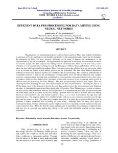
Figure 4. Regression tree on the neural network output.

(iii) neural network models with two to six nodes in the hidden layer (models 3–7); (iv) regression tree on the output of the neural network model with two hidden nodes (model 8); (v) regression tree on the raw data (model 9). For the proportional hazard models as well as the neural network model obtaining the log partial likelihood for the validation set is a direct evaluation of (3) or (5), respectively. However, for model 8, which involves the regression tree, we Brst grow the tree on the neural network output; the results are shown in Figure 4. After obtaining the tree, the appropriate risk groups were deBned. Table I summarizes the eight risk groups deBned by the regression tree. We see from Figure 4 and the risk groups deBned in Table I that, for example, for low values of creatinine the tree splits on di;erent variables and values than for high values of creatinine. Since the regression tree is grown on the output of the neural network these asymmetric splits in the tree and the associated risk groups reNect the high order interactions and or non-linearities that exist in the estimated neural network prediction model. With these risk groups deBned, binary dummy variables are easily constructed. Using these dummy variables in the proportional hazards model we estimated the parameters in the training set and evaluated the log partial likelihood results on the remaining two sets. Table II presents the log partial likelihood for the above models. Observing the results obtained for the validation set, the neural network model with two hidden nodes Copyright ? 2001 John Wiley & Sons, Ltd.

Statist. Med. 2001; 20:2965–2976

2972

D. FARAGGI, M. LEBLANC AND J. CROWLEY

Table I. Risk groups deBned by the regression tree on the neural network output. Risk group

Creatinine

Albumin

Age

1 2 3 4 5 6 7 8

¿4.2 1.85– 4.2 ¡1.85 ¡1.85 ¡1.85 ¡1.85 ¡1.85 ¡1.85

Any Any ¿4.05 3.75– 4.05 ¿3.75 2.85–3.75 2.85–3.75 ¡2.85

Any Any ¿56.5 ¿56.5 ¡56.5 ¿66.5 ¡66.5 Any

Table II. Log partial likelihood for the di;erent models. Model 1 2 3 4 5 6 7 8 9

PH 1st order PH 2nd order NN (h = 2) NN (h = 3) NN (h = 4) NN (h = 5) NN (h = 6) NN (h = 2) + trees Regression tree

Training

Stopping

Validation

−1178:23 −1175:24 −1183:35 −1180:92 −1177:27 −1178:10 −1172:72 −1180:92 −1173:93

−1148:34 −1148:99 −1146:79 −1148:14 −1145:56 −1148:21 −1145:70 −1158:32 −1164:81

−2050:28 −2053:35 −2043:72 −2045:85 −2044:05 −2046:67 −2045:47 −2064:76 −2066:72

(model 3) achieved the highest log partial likelihood among the models compared. It achieved a log partial likelihood of −2043:72 compared with the Brst- or the second-order proportional hazard models that achieved the value of −2050:28 and −2053:35, respectively. It should be noted that although the neural network model with two hidden nodes has 14 parameters while the Brst-order Cox model has only Bve parameters, the comparisons made above are done on the validation set, where the estimates should be considered constants. The neural network models (models 3–7) achieved similar results in terms of the log partial likelihoods for the validation set. Consequently we restrict ourselves to the simplest model with two hidden nodes. If model Btting for prediction of individual risks is desired, clearly this model is appropriate. However, when interpretable risk groups are desired, a regression tree on the output of the neural network is grown for the validation data; the log partial likelihood of that model (model 8) is −2064:76. As one should expect, using discrete risk groups instead of continuous covariates reduces the value of the log partial likelihood. Regression trees were extended to time until event data to facilitate the construction of groups of patients with di;erent prognoses [4; 26–29]. For survival data, evaluating the logrank test statistic and comparing the potential two subgroups is often used to choose the best split of the data. We have implemented the regression tree suggested by Crowley et al. [30] on these data as well and found the regression tree and the survival curves to be similar to those shown in Figures 4 and 5. The values of the log partial likelihood obtained from this model Copyright ? 2001 John Wiley & Sons, Ltd.

Statist. Med. 2001; 20:2965–2976

UNDERSTANDING NEURAL NETWORKS USING REGRESSION TREES

2973

Figure 5. Prognostic groups from neural net=tree. (a) training sample. (b) validation sample.

is −2066:72 (model 9). Again the result for the validation set for this model is very similar to the result obtained when the tree is grown on the output of the neural net (model 8). In addition to the risk groups deBned above we report in Figure 4 the average log relative risk for the di;erent subgroups. For example, patients with creatinine level higher than 4.2 had Copyright ? 2001 John Wiley & Sons, Ltd.

Statist. Med. 2001; 20:2965–2976

2974

D. FARAGGI, M. LEBLANC AND J. CROWLEY

the worst prognosis with average log relative risk of 0.95. The best prognosis was obtained for patients with creatinine level lower than 1.85, albumin level higher than 3.75 and with age less than 56.5. These patients achieved average log relative risk of −0:24. The histograms displayed below each terminal node provide a measure of the variability of the log relative risk estimates within each risk group. 5. DISCUSSION This paper presents a method of obtaining easily interpretable risk groups when one uses neural networks to model censored survival data. The purpose of obtaining these risk groups is to help us understand the scientiBc implications of the neural network model. This method is an alternative to the calculation of main e;ects and interaction presented by Faraggi and Simon [7]. Using their method, before estimating main e;ects and interactions, the user has to choose two values of any covariate to be considered ‘low’ and ‘high’. When continuous covariates are in the model it is sometimes di8cult to determine what values are ‘low’ and what values are ‘high’. In their example Faraggi and Simon [7] used the 25th and 75th quartile of any continuous covariate as representative values for ‘low’ and ‘high’, respectively. In cases when a covariate a;ects survival in a non-linear way, these may not be the best values to choose, neither is there any reason to expect that just two values should provide a su8cient split of the continuous covariates. The method of growing a regression tree on the neural network output overcomes these di8culties. It provides a Nexible way of understanding predictions using the neural network model and it also provides a natural way of splitting continuous covariates to form interpretable risk groups. If further simpliBcation of the model is desired, one can prune the regression tree displayed in Figure 4 using the method suggested by Breiman et al. [24] to obtain a regression tree with only four terminal nodes. Doing that we found two groups with similar survival curves. Consequently we amalgamated these patients into a single risk group to achieve three prognostic groups. The poor prognosis group includes patients having creatinine level higher than 4.2, the good prognosis group are the patients with creatinine level of less than 1.85 and albumin level higher than 3.75 and the intermediate risk group includes the rest of the patients. Survival curves of these three groups for both the training and validation sets are shown in Figures 5(a) and (b), respectively. Visual comparison of Figure 5(b) and the Durie–Salmon staging system displayed in Figure 1(a) shows a better separation of the survival curves on the validation set using the risk groups formed as described above. We have presented our method in the context of censored survival data. However, the use of neural network is not limited to such data. Growing regression trees on the output of a neural network can be easily implemented for continuous data in general to help interpret the importance of the variables and shown how they a;ect the neural network predictions. We have focused on the neural network model with only two nodes in the hidden layer. Neural networks are usually much more complex and involve many more parameters. As shown in Table II, these more complex models did not achieve higher log partial likelihood value on the validation set. From our experience with survival data [31; 32], the signal to noise ratio in these data sets is usually small, that is, large amount of noise compared to the signal. We Bnd that in many cases a neural network with a small number of nodes in the hidden layer is su8cient to explain the signal. Copyright ? 2001 John Wiley & Sons, Ltd.

Statist. Med. 2001; 20:2965–2976

UNDERSTANDING NEURAL NETWORKS USING REGRESSION TREES

2975

APPENDIX: GROWING AND PRUNING A REGRESSION TREE The Brst step in constructing a tree model is to consider the entire data set, and all feasible splits of the data are considered. Splits along co-ordinate axes are typically chosen because they are the easiest rules to interpret. For instance, for an ordered covariate the splits are of the form x1 63 versus x1 ¿3. The split that maximizes some improvement in model Bt G(h) = R(h) − (R(l(h) − R(r(h))) where R(h) is the residual error in node h and l(h) and r(h) represent the left and right data sets resulting from the split, is chosen. After splitting the data in two groups, each of the resulting groups is split again as before. The same rules are applied recursively until a moderate number of groups of patients are constructed. The partition can be represented as a binary tree, since only binary splits are used at each stage. Typically, the tree model that has been constructed is too complex to give good predictions. The performance of trees is usually indexed by the cost-complexity measure, which measures of the performance of the model Bt versus the tree complexity
R(h) + |T | R (T ) = h∈T

where R(h) is the residual error for observations falling into terminal node h. For large values of  small trees are preferred, and for small values of  large trees are produced. There is an e8cient algorithm to Bnd the pruned tree (tree obtained by removing branches) for any tree R (T0 ) = min{R(T
)} Since the same data were used to grow the tree as calculate the error, the error estimated can be quite biased. Therefore, cross-validation or other resampling methods have been developed to help select an appropriately sized tree. ACKNOWLEDGEMENTS

The authors thank the editor and two reviewers for helpful comments. REFERENCES 1. Cox DR. Regression models and life-tables. Journal of the Royal Statistical Society, Series B 1972; 34: 187–202. 2. Cox DR. Some remarks on the analysis of survival data. In Proceedings of the First Seattle Symposium in Biostatistics: Survival Analysis, Lin DY, Fleming TR (eds). Springer-Verlag: New York, 1997; 1–9. 3. KalbNeisch JD, Prentice RL. The Statistical Analysis of Failure Time Data. Wiley: New York, 1990. 4. LeBlanc M, Crowley J. Survival trees by goodness of split. Journal of the American Statistical Association 1993; 88:457– 467. 5. Durrleman S, Simon R. Flexible regression models with cubic splines. Statistics in Medicine 1989; 8:551–561. 6. Kooperberg C, Stone CJ, Truong YK. Hazard regression. Journal of the American Statistical Association 1995; 90:78–94. 7. Faraggi D, Simon R. A neural network model for survival data. Statistics in Medicine 1994; 14(1):73–82. 8. Dasgupta CG, Dispensa GS, Ghose S. Comparing the predictive performance of a neural network model with some traditional market response models. International Journal of Forecasting 1994; 10(2):235–244. Copyright ? 2001 John Wiley & Sons, Ltd.

Statist. Med. 2001; 20:2965–2976

2976

D. FARAGGI, M. LEBLANC AND J. CROWLEY

9. Prentice SD, Patla AE, Stacey DA. simple artiBcial neural network models can generate basic muscle activity patterns for human locomotion at di;erent speeds. Experimental Brain Research 1998; 123(4):474 – 480. 10. Salmon SE, Tesh D, Crowley J, Saeed S, Finley P, Milder MS, Hutchins LF, Coltman CA Jr., Bonnet JD, Cheson B, Knost JA, Samhouri A, Beckord J, Stoock-Novack D. Chemotherapy is superior to sequential hemibody irradiation for remission consolidation in multiple myeloma: A Southwest Oncology Group Study. Journal of Clinical Oncology 1990; 8:1575–1584. 11. Salmon SE, Crowley J, Grogan TM, Finley P, Pugh RP, Barlogie B. Combination chemotherapy glucocorticoids and intrerferon alpha in treatment multiple myeloma: A Southwest Oncology Group Study. Journal of Clinical Oncology 1994; 12:2405–2414. 12. Durie BGM, Salmon SE. A clinical system for multiple myeloma. Correlation of measured myeloma cell mass with presenting clinical features, response to treatment and survival. Cancer 1975; 36:842–854. 13. Rumelhart DE, Hinton GE, Williams RJ. Learning internal representations by error propagation. Parallel Distributed Processing 1986; 1:318–362. 14. Wasserman PD. Neural Computing Theory and Practice. Van Nostrand Reinhold: New York, 1989. 15. Cox DR. Partial likelihood. Biometrika 1975; 62:269–276. 16. Miller RG. Survival Analysis. Wiley: New York, 1981. 17. Lawless JF. Statistical Models and Methods for Lifetime Data. Wiley: New York, 1982. 18. Gallant AR, White H. On learning the derivatives of an unknown mapping with multilayer feedforward networks. Neural Networks 1991; 5:129–138. 19. Chauvin Y. Generalization performance of overtrained back-propagation networks. In Neural Networks, EURASIP Workshop. Springer-Verlag: 1990. 20. Geman S, Bienenstock E, Doursat R. Neural networks and the bias=variance dilemma. Neural Computation 1992; 4:1–58. 21. Smith M. Neural Networks for Statistical Modeling. Van Nostrand Reinhold: New York, 1993. 22. Ripley BD. Statistical aspects of neural networks. In Network and Chaos – Statistical and Probablistic Aspects, Brandor;-Nielsen OE, Jensen JL, Kendall WS (eds). Chapman and Hall: 1993. 23. Morgan JN, Sonquist JA. Problems in the analysis of survey data, and a proposal. Journal of the American Statistical Association 1963; 58:415– 434. 24. Breiman L, Friedman JH, Olshen RA, Stone CJ. Classi3cation and Regression Trees. Wadsworth: Belmont, CA, 1984. 25. Quinlin JR. C4.5 Programs for Machine Learning. Morgan Kaufman: 1993. 26. Gorden L, Olshen RA. Tree-structured survival analysis. Cancer Treatment Report 1985; 69:1065–1069. 27. Ciampi A, Thi;auld J, Nakache J-P, Asselain B. StratiBcation by stepwise regression, correspondence analysis and recursive partition. Computational Statistics and Data Analysis 1986; 4:185–204. 28. Ciampi A, Hogg S, Mckinney S, Thi;aut J. RECPAM: a computer program for recursive partition and amalgamation for censored survival data. Computer Methods and Programs in Biomedicine 1988; 26:239–256. 29. Segal MR. Regression trees for censored data. Biometrics 1988; 44:35– 48. 30. Crowley J, LeBlanc M, Jacobson J, Salmon SE. Some exploratory tools for survival analysis. In Proceedings of the First Seattle Symposium in Biostatistics: Survival Analysis, Lin DY, Fleming TR (eds). Springer-Verlag: New York, 1997; 199–229. 31. Mead GM on behalf of the IGCCCG. International Consensus Prognostic ClassiBcation for Metastatic Germ Cell Tumors Treated with Platinum Based Chemotherapy; A Bnal report of the International Germ Cell Cancer Collaborative Group (IGCCCG), ASCO, 1995. 32. Faraggi D, Simon R, Yaskil E, Kramar A. Bayesian neural network models for censored data. Biometrical Journal 1997; 39:519–532.

Copyright ? 2001 John Wiley & Sons, Ltd.

Statist. Med. 2001; 20:2965–2976