Académie de Montpellier

U n i v e r s i t é M o n t p e l l i e r II — Sciences et Techniques du Languedoc —

Thèse

pour obtenir le grade de

tel-00641678, version 1 - 16 Nov 2011

Docteur de l’Université Montpellier II

Discipline

:

Génie Informatique, Automatique et Traitement du Signal

Formation Doctorale

:

Systèmes Automatiques et Microélectroniques

École Doctorale

:

Information, Structures et Systèmes

présentée et soutenue publiquement par

Bruno Vilhena Adorno le 2 octobre 2011

Titre:

Two-arm Manipulation: From Manipulators to Enhanced Human-Robot Collaboration (Contribution à la manipulation à deux bras : des manipulateurs à la collaboration homme-robot)

Jury: Bruno Siciliano

Professeur, Università degli Studi di Napoli Federico II, Italie

Rapporteur

Masaru Uchiyama

Professeur, Tohoku University, Japan

Rapporteur

Oussama Khatib

Professeur, Stanford University, États-Unis

Examinateur

Philippe Fraisse

Professeur, Université Montpellier II, France

Directeur de thèse

Philippe Poignet

Professeur, Université Montpellier II, France

Examinateur

Véronique Perdereau

Professeur, Université Pierre et Marie Curie, France

Examinateur

tel-00641678, version 1 - 16 Nov 2011

T W O - A R M M A N I P U L AT I O N : F R O M M A N I P U L AT O R S T O E N H A N C E D H U M A N - R O B O T C O L L A B O R AT I O N

tel-00641678, version 1 - 16 Nov 2011

bruno vilhena adorno

Department of Robotics Laboratoire d’Informatique, de Robotique et de Microélectronique de Montpellier (LIRMM) Université Montpellier 2 October 2, 2011

tel-00641678, version 1 - 16 Nov 2011

Bruno Vilhena Adorno: Two-arm Manipulation: From Manipulators to Enhanced HumanRobot Collaboration (Contribution à la manipulation à deux bras : des manipulateurs à la collaboration homme-robot), © October 2, 2011

tel-00641678, version 1 - 16 Nov 2011

To Helena, Alice, and Polyana for standing by my side in this journey called life

tel-00641678, version 1 - 16 Nov 2011

tel-00641678, version 1 - 16 Nov 2011

ACKNOWLEDGMENTS

A PhD thesis is written by only one author, and sometimes this is a lonely task. It consists of many hours of intense thinking, struggling to understand and develop abstract (but hopefully useful) concepts, and trying to present them in a way that prepares the next scientist to further advance the theory and techniques introduced over a hundred pages. However, today my thesis exists, such as it is, and this is thanks to innumerable people. I once read somewhere that “behind a great man, there is always a great woman,” and I think that this could be rephrased as “behind a (great, or not) thesis, there are great people supporting the author.” This page is dedicated to them. First, I would like to thank Prof. Philippe Fraisse, who accepted me as his student. Always cordial in manner, he has never failed to show himself as open to discussion (technical or philosophical) and has provided me with the very best conditions to work in. Hard working and an exceptional project manager, he has participated in all aspects of my research—including the technical ones (which I think is quite rare among the supervisors of today)—and for this I am very grateful. His ethics and his way of living the academic life will always be a great source of inspiration. I would also like to thank Sébastien Druon and Stéphanie for helping me when I arrived in Montpellier. Their guidance made it much easier for me to navigate my way through the French bureaucracy. A special acknowledgement goes to Ahmed Chemori, Christine Azevedo, and Mitsuhiro Hayashibe. In addition to their agreeable presence in my daily life, they are models of hard workers—of people who make things happen. It is thanks to men and women like them that I continue to have great hope for the future of science. I cordially acknowledge Dr. Etienne Dombre for the very helpful remarks and encouragement he gave me whenever he was able to attend my presentations. I sincerely acknowledge Prof. André Crosnier and Prof. Philippe Poignet for their kindness and their faith in the “Brazilian team.” I cannot forget LIRMM’s administrative staff, in particular Nicole Gleizes and Olivier Minarro, who were never less than helpful and efficient. Without them, going to a conference would have been so much more difficult. Also, I would like to point out the remarkable job done by LIRMM’s technical staff. It’s thanks to their work behind the scenes that I was able to have all the infrastructure to execute my job. A special thanks goes to Prof. Véronique Perdereau for her cordiality and kindness. Our discussions about the project were all fruitful, and I was always warmly received in Paris. The same applies to Hoang-Lân Pham, with whom I have had the most stimulating discussions. This work wouldn’t be what it is without the keen remarks of Prof. Bruno Siciliano and Prof. Masaru Uchiyama. In addition to accepting to be reviewers of my thesis, their works have been an infinite source of inspiration. I’m sincerely grateful that Prof. Oussama Khatib accepted to be a member of my jury, despite his huge responsibility as the general chair of the IROS’11 conference. I am also thankful for the infrastructure he provided for my PhD defense at Stanford.

vii

tel-00641678, version 1 - 16 Nov 2011

I would like to thank Catherine Carmeni for helping to improve the text and my English writing. She did a remarkable job of transforming a barbarian text into a decent one, always with great efficiency and professionalism. The time that I spent in the lab wouldn’t have been so pleasant if the other PhD students hadn’t been present. The mix of cultures and ideas definitely has made me a better person. Even at the risk of forgetting to acknowledge some of my colleagues and friends (if I do forget, I will make it up to them by offering “pamonha”, “pão de queijo”, and “cachaça” in Belo Horizonte, I promise), I must write down a list of the important people who shared their friendship with me over these last three years: Alain Hassoun, Ashvin Sobhee, Azhar Hadmi, Baptiste Magnier, Bastien Durand, Chao Liu, Dalila Goudia, Guilherme Bontorin, Jean Da Rolt, João Azevedo, Johann Lamaury, Luis Vitorio Cargnini, Nabil Zemiti, Naveed Islam, Nicolas Carlesi, Nicolas Philippe, Nicolas Riehl, Pattaraporn Warintarawej, Pawel Maciejasz, Raphael M. Brum, Renan Alves Fonseca, Roseline Bénière, Sébastien Cotton, Sébastien Krut, Vincent Bonnet, and Zeineb Zarrouk. My heart will always have a special place for good friends: Alfredo (compadre) Toriz Palacios, Andreea (niña) Elena Ancuta, Divine Maalouf, Giulia Toncelli, Guilherme Sartori Natal, Hai Yang, Jovana Jovic, Lama (Lamex) Mourad, Lotfi (rio de janeeeeiro) Chikh, Luis Alonso (Banderas) Sánchez Secades, Michel Dominici, Michele Vanoncini, Mourad Benoussad, Pedro Moreira, Qin Zhang, and Xianbo Xiang. It is very difficult to express in words my gratitude for these most cherished friends: Antônio P. L. Bó, Mariana C. Bernardes, Carla S. R. Aguiar, and Rogério Richa. We’ve been good friends for many years, and I’m proud to say that they are part of my family. Outside the lab, dear friends have become part of my life: Gabriel, Bruna and little João Gabriel (you’ll have to bring João to visit Alice!) and Luiz and Denise. I have missed my family in Brazil terribly these last three years, and I’m grateful that they were able to understand and graciously accept my absence. Their support has been so important to me. Last, but most importantly, I would like to thank my wife Polyana and our two wonderful daughters, Alice and Helena. These three girls definitely make me feel fulfilled, and with them standing by my side, life is worth living.

viii

CONTENTS List of Figures xi List of Tables xii Acronyms xiii Notation and conventions xiv introduction 1 state of the art 5 1.1 Multi-arm manipulation 8 1.1.1 Augmented object and virtual linkage 9 1.1.2 Symmetric control scheme 11 1.1.3 Cooperative task-space 12 1.1.4 Synchronized control 14 1.1.5 Other representations 15 1.2 Conclusion 16 2 kinematic modeling using dual quaternions 19 2.1 Mathematical background 20 2.1.1 Quaternions 21 2.1.2 Dual numbers 23 2.1.3 Dual quaternions 24 2.2 Rigid body motion 26 2.2.1 Rotations represented by quaternions 26 2.2.2 Rigid motions represented by quaternions 28 2.2.3 Rigid motions represented by dual quaternions 28 2.2.4 Decompositional multiplication 30 2.3 Robot kinematic modeling 36 2.3.1 Forward kinematic model 36 2.3.2 Dual quaternion Jacobian 38 2.4 Dual quaternions vs. homogeneous transformation matrices 41 2.4.1 Forward kinematic model 41 2.4.2 Jacobian 43 2.4.3 Decompositional multiplication 45 2.5 Conclusion 46 3 two-arm manipulation: the cooperative dual task-space approach 3.1 The cooperative dual task-space: arm coordination 50 3.2 Cooperative Jacobians 52 3.2.1 Preliminaries 53 3.2.2 Relative dual quaternion Jacobian 54 3.2.3 Absolute dual quaternion Jacobian 54 3.3 Cooperative dual task-space: object manipulation 56 3.3.1 Preliminaries 56 3.3.2 Wrenches and twists in the cooperative dual task-space 60 3.3.3 Complete description of the cooperative dual task-space 62

tel-00641678, version 1 - 16 Nov 2011

1

49

ix

tel-00641678, version 1 - 16 Nov 2011

x

contents

3.4 Kinematic control in the cooperative dual task-space 67 3.5 Control primitives 72 3.6 Conclusion 81 4 two-arm mobile manipulation: the cooperative dual task-space approach 83 4.1 Serially coupled kinematic structure 84 4.2 Extended cooperative dual task-space 86 4.3 Case study: two-arm mobile manipulator 88 4.4 Simulation results and discussions 90 4.5 Conclusion 94 5 human-robot cooperation: the cooperative dual task-space approach 95 5.1 Intuitive task definition 96 5.2 Robot’s perception of the human motion 97 5.3 Control of the robot arm 97 5.4 Control of the human arm 98 5.4.1 Human arm control by using functional electrical stimulation 98 5.4.2 Human arm control in the Cartesian space 99 5.5 Experiments 101 5.5.1 Water pouring 101 5.5.2 Teleoperation 102 5.5.3 Simultaneous handling using mirrored movements 103 5.5.4 Ball in the hoop 105 5.6 Conclusion 108 6 conclusion and perspectives 113 Appendix 115 a general mathematical facts, definitions, and properties 117 a.1 Dual number properties 117 a.2 Quaternion properties 117 a.3 Properties of Hamilton operators 120 a.4 Dual quaternion properties 121 a.4.1 Unit dual quaternions and rigid motions 122 a.5 Properties of the generalized Jacobian 124 a.6 Properties of the decompositional multiplication 125 b denavit-hartenberg parameters of the robots 127 c experimental setup for the human-robot collaboration 129 c.1 “Teleoperation with collaboration” experiment 129 c.2 “Water pouring” and “mirrored movements followed by simultaneous handling” experiments 130 c.3 Calibration procedure for the “ball in the hoop” experiment 131 Bibliography 133 Publications 141 Index 143

LIST OF FIGURES

Figure 1 Figure 2

tel-00641678, version 1 - 16 Nov 2011

Figure 3 Figure 4 Figure 5 Figure 6 Figure 7 Figure 8 Figure 9 Figure 10 Figure 11 Figure 12 Figure 13 Figure 14 Figure 15 Figure 16 Figure 17 Figure 18 Figure 19 Figure 20 Figure 21 Figure 22 Figure 23 Figure 24 Figure 25 Figure 26 Figure 27 Figure 28 Figure 29 Figure 30 Figure 31 Figure 32 Figure 33 Figure 34 Figure 35 Figure 36

First CAD design of the ASSIST robot, made by CEA. 2 Humanoid robots which can potentially work side-by-side with humans. 6 Two-arm mobile manipulators: PR2 and Twendy-one. 7 Justin and ARMAR-III. 8 Augmented object model. 10 Virtual linkage. 10 Two-arm manipulation using the symmetric control representation. 12 Synchronized interaction between two mobile manipulators. 15 Rotation represented by a quaternion. 26 Frame rotation represented by quaternions. 27 Point rotation represented by quaternions. 27 One rigid motion represented by quaternions. 28 Sequence of rigid motions represented by quaternions. 29 Robot hand manipulating a screwdriver. 31 Standard versus decompositional multiplication. 32 The “frame in the box“ example. 35 Denavit-Hartenberg parameters 37 Cooperative dual task-space representation. 51 Manipulating a broom. 52 Wrenches and twists represented by dual quaternions. 56 Cooperative dual task-space: manipulation of a firmly grasped object. 61 Initial and final configurations for the KUKA arm 69 Error of each dual quaternion coefficient. 69 Trajectory executed by the KUKA arm. 70 Two KUKA LWR 4 manipulating a broom. 71 Coefficients of the relative dual quaternion of example 3.4 73 Coefficients of the absolute dual quaternion of example 3.4 74 Angle between the robotic hands in the task of manipulating a broom. 74 Relative translation between the robotic hands in the task of manipulating a broom. 75 Two-arm manipulation of a large box. 75 Manipulation of Rubik’s cube. 75 Opening a bottle. 76 Turning a driving wheel. 76 Positioning a screw driver. 78 Manipulation of a flashlight. 78 Two-arm manipulation: grabbing a balloon. 79

xi

Figure 37 Figure 38 Figure 39

tel-00641678, version 1 - 16 Nov 2011

Figure 40 Figure 41 Figure 42 Figure 43 Figure 44 Figure 45 Figure 46 Figure 47 Figure 48 Figure 49 Figure 50 Figure 51 Figure 52 Figure 53 Figure 54 Figure 55 Figure 56 Figure 57 Figure 58

Two-arm manipulation: task of pouring water. 80 Serial kinematic system composed by several intermediate subsystems. 85 Serially coupled kinematic chain for a two-arm mobile manipulator. 88 Sequence corresponding to the reaching phase in the task of pouring water. 92 Task of pouring water using the whole body motion. 93 Examples of cooperative tasks. 97 Experimental setup for the human-robot collaboration. 98 Actuation of the human arm: positioning of the electrodes. 100 The human arm modeled as a one-link serial robot. 100 Task of pouring water. 102 Teleoperation with collaboration. 102 Sequence of human-robot collaboration (HRC) in mirror mode. 104 Constrained movement in the ball in the hoop experiment. 105 Coordinate systems in the ball in the hoop experiment. 106 Sequence of one trial in the ball in the hoop experiment. 109 Time response for the successful trial shown in figure 51. 110 Number of trials versus individual performance. 110 Impact of the cooperation in the success of the task. 110 Comparison of the success rate. 111 Plücker line. 123 Plücker line with respect to frames Fa and Fb . 124 Representation of the frames in the “teleoperation with collaboration” task. 130

L I S T O F TA B L E S

Table 1 Table 2 Table 3 Table 4 Table 5 Table 6 Table 7 Table 8 Table 9

xii

Cost comparison between homogeneous transformation matrices and dual quaternions. 43 Summary of control primitives and correspondent task Jacobians. 78 Extended absolute Jacobian. 90 Definition of the task of pouring water. 91 Denavit-Hartenberg (D-H) parameters for the human arm. 101 Parameters of the cooperative tasks. 104 Criteria used to evaluate the ball in the hoop task. 107 Standard D-H parameters of the KUKA LWR 4 (Giordano, 2007). 127 Modified D-H parameters of the Hoap-3’s arms. 127

acronyms

tel-00641678, version 1 - 16 Nov 2011

ACRONYMS

ASIMO

Advanced Step in Innovative MObility

CAD

computer-aided design

CEA

Commissariat à l’énergie atomique et aux énergies alternatives

D-H

Denavit-Hartenberg

DLR

German Aerospace Center

DOF

degrees of freedom

FKM

forward kinematic model

FES

functional electrical stimulation

HRI

human-robot interaction

HRC

human-robot collaboration

ISIR

Institut des Systèmes Intelligents et de Robotique

LAAS

Laboratoire d’Analyse et d’Architecture des Systèmes

LIRMM

Laboratoire d’Informatique, de Robotique et de Microélectronique de Montpellier

NASA

National Aeronautics and Space Administration

PRM

Probabilistic Roadmap

ROS

Robot Operating System

xiii

tel-00641678, version 1 - 16 Nov 2011

N O TAT I O N A N D C O N V E N T I O N S

Lowercase plain letters represent scalars. For instance, a = 1, b = −0.333. The variables i, j, l, m, n always denote integers.

tel-00641678, version 1 - 16 Nov 2011

The hatted variables ıˆ, ˆ, kˆ denote imaginary units. The following sets are used throughout the thesis: – R : set of real numbers – H : set of quaternions – H: set of dual quaternions Lowercase bold letters represent column vectors or quaternions:     b1 a1  .   .   .  .  a, b ∈ Rn a=  . , b =  . , bn an

or

ˆ 4, c = c1 + ˆıc2 + ˆc3 + kc

Uppercase bold letters usually represent matrices:  a11 · · · a1n  . .. ..  A =  .. . . a1m · · · amn

c ∈ H.



 , 

with the exception of F and M, which are column vectors representing forces and moments, respectively. Underlined variables represent dual numbers. For instance, a = a1 + εa2 is a dual scalar whereas h = h1 + εh2 is a dual quaternion, where ε is the dual unit. The letter T is reserved to denote the transpose of matrices and vectors; for instance, AT is the transpose of A. Coordinate systems are represented by Fref , where ref can be any label representing the name of the coordinate system; for example, F1 and Fworld . If the coordinate system is

xv

xvi

notation and conventions

not important, usually the subscript is omitted, e.g., F. Rotation matrices representing the rotation from frame i to frame j are given by Rij . If they are given with respect to a general reference frame or the reference frame is not defined, the superscript is omitted; for instance, Rj . The same apply to vectors; that is, when the reference frame is not defined or all the quantities are related to the same reference frame, the superscript can be omitted. For instance, the velocities v1 and v2 are given with respect to the same reference frame (which is not specified), but va 1 and vb are given with respect to F and F , respectively. a b 2

tel-00641678, version 1 - 16 Nov 2011

The same rule applies for homogeneous transformation matrices, quaternions and dual quaternions; that is, Hij represents the homogeneous transformation from frame i to frame j, the quaternion rij represents the rotation from frame i to frame j, and the dual quaternion xij represents the rigid motion from frame i to frame j. Physical variables, such as position, velocity, force, and so on, are represented—unless explicitly stated otherwise—by quaternions; for example, the velocity v is represented ˆ z . Only chapter 1 does not follow this rule. by the quaternion v = ˆıvx + ˆvy + kv Dual positions, twists, and wrenches are represented by dual quaternions, and usually the symbols x, ξ, and f are used to represent each one of these physical entities, respectively. Matrices corresponding to task Jacobians are represented by J. Subscripts are usually used to denote the controlled task. J+ and J† denote the Moore-Penrose pseudoinverse and the damped least-square inverse of the matrix J, respectively. G is the generalized Jacobian. Gain matrices are usually represented by K, whereas scalar gains are usually represented by λ. Re (x) and Im (x) denote the real and imaginary parts of the quaternion x. The same applies for dual quaternions. h iT ım = ıˆ ˆ kˆ is the imaginary vector unit. ε is the dual unit.

Given the dual quaternion x: +

−

– H (x) and H (x) are the Hamilton operators of x. – P (x) and D (x) denote the primary and secondary parts of x. – x∗ is the conjugate of x.

notation and conventions

– The operator vec x performs the mapping of x into R8 . The symbol ⊗ denotes the decompositional multiplication. The symbol × represents the cross product between pure quaternions (the ones with real parts equal to zero). For instance, a × b, a, b ∈ H, is the cross product between the ×

quaternions a and b, which is equivalent to H (a) vec b (see appendix A).

tel-00641678, version 1 - 16 Nov 2011

a The dual quaternion xa b raised to the n-th power is denoted by xb ets are used to prevent mixing the power n with the superscript a.


{n}

. The curly brack-

xvii

tel-00641678, version 1 - 16 Nov 2011

tel-00641678, version 1 - 16 Nov 2011

INTRODUCTION

The robots of today are no longer confined to structured environments. As a result of fifty years of research, we are seeing increasingly more robots outside of factories, ranging from unmanned marine and aerial robots (Marani et al., 2010; Cheng et al., 2009) to robots in human environments (Kemp et al., 2007) like hospitals (Hockstein et al., 2007), and even robots capable of traveling across the desert (Thrun et al., 2006) and robots connected to the internet (Tenorth et al., 2011). With this paradigm shift, the research in assistive and “human-centered” robotics has become more intensive, and new challenges are now being faced. For instance, although robots and humans do not usually share the same workspace in factories, assistant robots do physically interact with people, which poses some safety constraints. Also, industrial robots must execute tasks that are usually completely described. In humanrobot interaction (HRI), however, the description of the task is often incomplete; for example, the order “give me the small bottle of water” implies recognizing a small bottle containing water. How is small defined in this case, and how can a bottle of water be differentiated from a bottle of tequila? A closer analysis of this simple task can shed some light on its inherent difficulties. Indeed, the localization and tracking of even fully-described simple objects in cluttered environments require robust computer vision algorithms. Also, in order to grasp a distant object the robot must navigate without colliding with obstacles across the environment to reach the desired object. Still considering the “give me the small bottle of water” task, suppose that the object is located, grasped and brought to the person who commanded the robot. The robot then must safely give the bottle to the person. How should the bottle be handed over? When should the robot release the bottle? What if the person moves while the robot is making the transfer? What if the person says “open the bottle”? Although there is still considerable work being done (and to be done) in computer vision, some good and stable software libraries are fortunately available (Marchand et al., 2005; Bradski & Kaehler, 2008). Navigation and motion algorithms are quite mature nowadays (Choset et al., 2005). Moreover, with the advent of software architectures like Robot Operating System (ROS) 1 and Orocos 2 , the integration of navigation and motion algorithms into robotic platforms now tends to be widespread. Daily domestic household tasks are usually easily performed by healthy youths but, despite recent advances, robots are not capable of performing them effectively(Kemp et al., 2007). The challenges of assistive robotics are even more accentuated when robots must assist the elderly or individuals with impairments. These people often have motion limitations that need to be taken into consideration at the moment of physical humanrobot interaction (e.g., tremor, absence of motion, and so on). The above examples showed that even the “simplest” of tasks can be very challenging for robots. The “give me the small bottle of water” task is usually considered simple because humans generally perform it naturally. But these tasks are challenging for robots 1. http://www.ros.org/ 2. http://www.orocos.org/

1

tel-00641678, version 1 - 16 Nov 2011

2

introduction

Figure 1: First CAD design of the ASSIST robot, made by CEA.

because, unlike humans, robots are not the product of a very long evolutionary process. At least for the moment, there is plenty of room for robotics research. This thesis was developed within the context of the ASSIST project. The aim of this project is to build a two-arm mobile manipulator to assist quadriplegic individuals in their daily lives. It has five partners (Commissariat à l’énergie atomique et aux énergies alternatives (CEA), Institut des Systèmes Intelligents et de Robotique (ISIR), Laboratoire d’Analyse et d’Architecture des Systèmes (LAAS), Laboratoire d’Informatique, de Robotique et de Microélectronique de Montpellier (LIRMM), and Propara Clinical Center) working together in order to push the frontiers of the state of the art in assistive robotics. The principles that have guided the robot design are safety, dexterity and capabilities of human-robot interaction. The ASSIST robot, depicted in figure 1, is composed of a mobile base, two arms with seven degrees of freedom (DOF) each, and a torso with one DOF. The robot should be capable of performing simple tasks such as locating and grasping simple objects, handing over objects to a person, and opening a bottle. Although the aforementioned tasks are quite trivial for a healthy person, reliable robotic implementations of these features is still a challenge. Because there are still many open questions in robotics and much to improve in its current techniques, it is humanly impossible to tackle them all. From the point of view of practical applications, this thesis is thus focused mainly on two-arm manipulation and its application to mobile manipulators and HRC. Two-arm manipulation is particularly interesting from both practical and theoretical points of view. From the practical side, bi-manual tasks are constantly required over the course of a typical day, and a successful assistant robot must be skilled in these types of manipulation. From a theoretical point of view, two-arm manipulation poses several challenges. First, a suitable description for two-arm coordination should be sim-

introduction

ple enough to enable generalizations; that is, different tasks should be easily defined without any modification in the original description, and the final formalism should be easily extended to more complex robots (e.g., mobile manipulators, humanoids, and so on). Also, this description should take into account not only the bi-manual tasks executed by the robot, but also the bi-manual tasks involving different agents, such as handing over, pouring water, and so on. Because the robot must interact with humans, the two-arm coordination should also be reactive. For these reasons, the techniques developed in this thesis tend to be low-level oriented. Last, departing from the requirements imposed by the ASSIST project, I was also interested in some fundamental aspects related to the foundations of robotics; notably, the unification of robot kinematic modeling and control by means of dual quaternions.

contributions

tel-00641678, version 1 - 16 Nov 2011

The contributions of this thesis are divided into three main groups: 1. The robot kinematic modeling is unified with kinematic control by means of dual quaternions, and a method for obtaining the forward kinematic model (FKM) and the differential FKM of serial robots is proposed, as well as kinematic controllers that directly use the dual quaternion as the input. 2. A generalized two-arm manipulation formalism is developed based on previous techniques from Uchiyama & Dauchez (1988), Chiacchio et al. (1996), and Caccavale et al. (2000). The representation of two-arm manipulation is first unified by means of dual quaternions; that is, dual positions (positions and orientations), twists (linear and angular velocities), and wrenches (forces and moments) are all represented in dual quaternion space. The formalism is then extended in order to take into account any serially coupled kinematic robot; for instance, mobile manipulators. 3. Techniques for intuitive human-robot collaboration are developed, such that conceptually different tasks can be represented by the same set of equations. Tasks like pouring water, teleoperation with collaboration, simultaneous handling, and mirrored movements are all represented within the two-arm manipulation formalism. In this manner, bimanual tasks previously designed to be executed by robots can be performed cooperatively between humans and robots. In addition, a novel application of human-robot collaboration is proposed, where the robot controls not only its arm, but also the human arm by means of functional electrical stimulation (FES). This application opens a new door toward novel interactions between robots and impaired individuals (e.g., quadriplegics). In addition to presenting the organization of the thesis, the next section highlights the contributions, chapter by chapter.

organization of the thesis The thesis is organized into six chapters, summarized as follows:

3

tel-00641678, version 1 - 16 Nov 2011

4

introduction

Chapter 1 presents some of the most recent developments in bimanual robots designed to work side-by-side with humans. Also, the mainstream two-arm manipulation techniques are revisited in order to provide the foundations on which this thesis is built. Chapter 2 first introduces the mathematical background needed to understand the concepts proposed throughout the thesis. Readers should read this chapter carefully, as it also establishes the notation and the overall nomenclature. Also, it proposes a novel operation, the decompositional multiplication, which aims to represent rigid motions that are invariant with respect to the pose of the modified frame. The chapter further proposes robot kinematic modeling by using dual quaternions. Although robot kinematics has been extensively studied over the past forty years, this chapter presents another point of view on the subject. Last, dual quaternions and homogeneous transformation matrices are compared in terms of the number of the elementary operations required by each representation. Chapter 3 proposes a new approach, the cooperative dual task-space, based on dual quaternions for bimanual manipulation. Inspired by some of the works reviewed in chapter 1, a complete description of two-arm coordination/manipulation is developed, by using dual quaternions, in terms of the dual positions, twists, and wrenches involved in the bimanual task. Furthermore, the chapter proposes techniques of kinematic control based entirely on the dual quaternion representation, and techniques designed for redundant robots are revisited in the context of the cooperative dual task-space. Last, control primitives are proposed in order to ease the definition of tasks. Chapter 4 proposes a generalization of the cooperative dual task-space in order to take into account whole-body motions. A case study using a simulated two-arm mobile manipulator is presented. Chapter 5 proposes a novel application of the cooperative dual task-space in the description and control of human-robot collaboration tasks. It shows that tasks that are usually regarded as conceptually different can be represented by the same set of equations and thus are mathematically equivalent. Last, a new approach in human-robot collaboration is proposed, where the robot controls not only its arm, but also the human arm by means of FES. This new approach can potentially be applied to novel interactions between robots and disabled people. Chapter 6 presents the concluding remarks and perspectives for future works.

note about the language and style This thesis follows the guidelines of the Chicago Manual of Style for English (The University of Chicago, 2010). This style, also adopted by the IEEE, does not condemn the use of the first person in scientific texts and thus differently somewhat from accepted style in some of the Latin languages, such as Portuguese and French. As a result, the first person singular is used in this thesis, although sparingly, to express my opinions or personal choices. On the other hand, the editorial “we” is never used, as the thesis was written by only one person. Therefore, whenever “I” appears in the text, the reader should read “the author of this thesis.” On the other hand, if “we” is used in the text, it will always be the inclusive “we”; that is, the readers should read “the author of this thesis and I (the reader).”

1

tel-00641678, version 1 - 16 Nov 2011

S TAT E O F T H E A R T

The dream of having robots to serve and help humans has a long history and is deeply embedded in the popular imagination. This dream is amply reflected in the large number of Hollywood movies and science fiction books on the human-robot relationship. Some of them are apocalyptic, with machines fighting against humanity, whereas others portray robots as gently helping people by means of high intelligence and motor dexterity. The common characteristic of such diametrically opposed visions is the huge capacity of robots to interact with humans and to autonomously solve tasks that should normally be solved only by intelligent beings. Although humanity has not reached this utopia, over the past forty years engineers, scientists, psychologists, mathematicians, and others have collectively been working to build robots capable of helping people in several types of tasks and fields. Today we can see, for example, rehabilitation and healthcare robots, domestic robots, robots for hazardous applications, and so on (Siciliano & Khatib, 2008). For robots that interact closely with humans and/or in human environments, anthropomorphic structures have always had an elevated status compared with non-anthropomorphic counterparts. One reason is that “human tools match human dexterity” (Kemp et al., 2008). This means that humans design and build environments and tools suitable for human beings. Thus, one might expect that the more a robot is similar to humans, the fewer the modifications needed in the environment and/or tools in order to use the robot effectively. Furthermore, humanoids and anthropomorphic designs facilitate the interaction between an individual person and the robot, since people are used to working with other people (Kemp et al., 2008). Several humanoid robots have already been designed to assist and interact with people. One of the most famous is Advanced Step in Innovative MObility (ASIMO), whose ultimate goal is to support human daily activities (Sakagami et al., 2002). ASIMO, shown in figure 2a, has some quite impressive abilities, being able, for example, to recognize people by means of a visual and auditory system and to interact with them by using gestures and a speech synthesis system. It can navigate in indoor environments, avoiding obstacles and using stairs, and plan its actions by using a behavior-based planning architecture (Sakagami et al., 2002). Another robot, Robonaut (Bluethmann et al., 2003), was primarily designed to work in outer space, as it is capable of cooperating with humans in tasks such soldering and taking electrical measurements. Although designed within a teleoperation framework, Robonaut has some degree of autonomy. As it has a vision system capable of tracking people and common tools like wrenches, it can search for a requested object by using voice recognition and give it to a human companion. Robonaut’s second generation, Robonaut 2 (fig. 2b), is a robot with 42 DOF capable of using tools designed for humans (Diftler et al., 2011). This robot was jointly developed by National Aeronautics and Space Administration (NASA) and General Motors, being the first humanoid to be in outerspace. In the robot design, human-robot interaction

5

tel-00641678, version 1 - 16 Nov 2011

6

state of the art

(a)

(b)

(c)

Figure 2: Humanoid robots which can potentially work side-by-side with humans: (a) ASIMO (courtesy of Honda), (b) Robonaut 2 (courtesy of NASA), and (c) HRP-2 (courtesy of AIST-CNRS).

aspects were paramount. For instance, the robot makes use of series elastic actuators, exhibiting large shock tolerance and accurate and stable force control. Furthermore, it uses an impedance-based control system that limits the force that the robot applies to the environment, thus making it suitable to work side-by-side with humans (Diftler et al., 2011). A very popular humanoid, the HRP-2 (fig. 2c), has also been used to evaluate the capabilities of humanoids in assisting humans. For instance, Okada et al. (2005) developed a complete software system for HRP-2 and showed the impressive capabilities of this robot in a kitchen environment. The robot is capable of navigating through the environment while moving obstructing objects (e.g., chairs) whenever necessary. The robot is equipped with a vision system, as well as several layers of motion and action planners. The motion planners take into account stability constraints, as well collision avoidance with the environment. Okada et al. (2005) performed an experiment where the robot was capable of recognizing a teapot, then poured water into a nearby cup, and finally navigated while carrying a tray with the cup on it. One drawback of using humanoid robots is that balance control must be ensured. Although there have been considerable advances in this field, humanoids still do not have good enough balance control to interact safely with people—mainly those with impairments—in realistic scenarios. Indeed, the great majority of big humanoids are confined to laboratory environments and they are operated while attached to chain belts to avoid damage due to falling. Other robots, mobile manipulators, have been developed to work in human environments. Willow Garage’s PR2, shown in figure 3a, integrates several software components, such as navigation, perception, manipulation, motion planning, and so on, on

tel-00641678, version 1 - 16 Nov 2011

state of the art

(a)

(b)

Figure 3: Two-arm mobile manipulators: (a) PR2 (Courtesy of Willow Garage); (b) Twendy-one (Courtesy of Sugano Laboratory, WASEDA University).

top of the Robot Operating System (ROS). PR2 is capable of fetching drinks, navigating and opening doors, and plugging itself into power outlets (Bohren et al., 2011). The huge complexity inherent to placing such an amount of heterogeneous components is alleviated by the use of ROS. Specifically designed with the elderly Japanese woman in mind, Twendy-one (fig. 3b) is capable of “helping the sitting-up motion support, transfering the caretaker onto a wheelchair and manipulating kitchen tools to make the breakfast” (Iwata & Sugano, 2009). Thanks to its 4-DOF torso, Twendy-one can pick up objects from the floor. Also, the passivity-based mechanisms for the robot arms enable safe interaction with humans and the environment. Because of this passivity, the arms can absorb the external forces arising from imprecisions in position control. Rollin’ Justin (fig. 4a), currently one of the most popular two-arm mobile manipulators, “is designed for research on sophisticated control algorithms for complex kinematic chains as well as mobile two-handed manipulation and navigation in typical human environments“ (Borst et al., 2009). This robot was developed by German Aerospace Center (DLR) and can be used for safe human-robot interaction because of the impedance behavior on joint, end-effector, and object levels. Using two of DLR’s lightweight arms and an advanced computer vision system, Rollin’ Justin is capable of fine manipulation (e.g., in the task of preparing coffee (Schmidt et al., 2011)), dexterous two-arm manipulation (Ott et al., 2006), and even catching flying balls (Schmidt et al., 2011). Another robot, ARMAR-III (fig. 4b), is also capable of performing complex tasks in household environments. For instance, ARMAR-III can recognize cups, dishes, and boxes of any kind of food, and it can automously load and unload a dishwasher with different kind of objects—e.g., tetra packs, bottle with tags, etc (Asfour et al., 2006).

7

tel-00641678, version 1 - 16 Nov 2011

8

state of the art

(a)

(b)

Figure 4: Two-arm mobile manipulators: (a) Justin (Courtesy of DLR); (b) ARMAR-III (courtesy of Karlsruhe Institute of Technology).

The aforementioned robot systems demonstrate an important point: in order to share the same environment with humans, robots must be adapted for human environments and for using human tools. Dexterous manipulation turns out to be crucial in these robot systems. Moreover, because two-arm manipulation offers possibilities in terms of dexterous manipulation (e.g., carrying large payloads, opening bottles), successful assistant robots must be skilled in this kind of manipulation. The next section presents the state of the art and mainstream techniques used to represent and perform multi-arm manipulation.

1.1

multi-arm manipulation

In the past thirty years,considerable research has been conducted on multi-manipulator systems (Caccavale & Uchiyama, 2008). This kind of cooperative system—of which twoarm manipulation is a particular case—can be used to carry heavy payloads and perform complex assembly tasks (Caccavale & Uchiyama, 2008). However, these advantages come with the drawback of having a more complex system. For instance, multiple manipulators cause internal stresses in the manipulated object, and typically a force control scheme has to be used in order to minimize these forces. The following sections present the main approaches proposed to tackle the problem of multi-arm manipulation.

1.1 multi-arm manipulation

1.1.1 Augmented object and virtual linkage

tel-00641678, version 1 - 16 Nov 2011

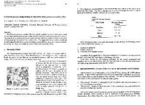
Khatib (1988) presented a control scheme using N robots with m-DOF each and rigidly connected to a common manipulated object. Khatib called the resultant system—that is, the end-effector plus the object—the augmented object, since the description of the overall system takes into account the inertial characteristics of all the effectors and the object. This augmented object is submitted to an operational 1 force fO at the operational point xO , as shown in figure 5. The operational force fO is the resultant of the contribution of each of the end-effectors’ wrenches. Considering the constraints of the augmented object model, Khatib wrote the system’s equations of motion analogously to his operational space formulation (Khatib, 1987), providing an elegant generalization of the operational space: fO = Λs (xO ) x¨ O + Πs (xO ) [x˙ O x˙ O ] + ps (xO ) , where Λs (xO ) is the kinetic energy matrix, Πs (xO ) is the matrix of the centrifugal and Coriolis forces 2 and ps (xO ) is the gravity vector. The subscript s stands for the N-effector/object system, implying that the aforementioned matrices and gravity vector take into account the object and all N-effectors. In order to control the augmented object, Khatib proposed the control structure cs (xO ) fod + Π cs (xO ) [x˙ O x˙ O ] + p cs (xO ) , fO = Λ

cs , Π cs , and p cs are the estimates of the respective matrices, and fod is the desired where Λ operational force. This control structure considers the net value of the operational forces. However, to allocate the individual effector forces, Khatib imposed the condition that the forces fOi produced by each effector would be aligned with fO ; that is, f O i = αi f O ,

(1.1)

resulting in the following vector of joint forces: τi = αi JTi fOi ,

(1.2)

where Ji is the geometric Jacobian of the i-th manipulator and αi is chosen such that the effort is equally distributed among the manipulators. Eq. (1.1) and (1.2) show two important consequences: first, the system is not capable of handling internal forces (i.e., forces that do not produce movements, only internal stresses in the manipulated object) and, second, the system requires torque-actuated robots, which are not always available. In order to control the internal forces and moments, Williams & Khatib (1993) proposed a physical model for these internal stresses that appear in multi-arm manipulation. This model is based on a virtual linkage between the grasping points, as shown in figure 6. Acknowledging that forces cause stress throughout the object, whereas moments cause local stress, Williams & Khatib separated the kinematic structure of the virtual linkage into two elements. The first element is a prismatic joint to represent the 1. In Khatib’s nomenclature, the operational force is a wrench (the vector containing force and moment) applied at the operational point. Moreover, the vector xO representing the generalized coordinates of the operational point contains information of position and orientation. h i

˙ stands for 2. In Khatib’s symbolic notation, [x˙ x] xi . . . xm are the coordinates of the operational point.

x˙ 21

2x˙ 1 x˙ 2

...

2x˙ 1 x˙ m

x˙ 22

...

x˙ 2m , where

9

10

state of the art

f3

fO

tel-00641678, version 1 - 16 Nov 2011

f1

f2 xO

Figure 5: Augmented object model: the forces and moments fi at the i-th end-effector are aligned with the operational force fO . Using only this model, the internal forces cannot be controlled.

Figure 6: Virtual linkage: spherical joints at each grasp represent internal moments, whereas prismatic joints between two end-effectors represent internal forces.

internal forces due to the interaction between two arms. The second element, representing the internal moments caused by each actuator, is a spherical joint connecting the prismatic joints, as illustrated in figure 6.

1.1 multi-arm manipulation

The relationship expressing the resultant (fres ) and internal (fint ) wrenches in terms of applied forces and moments at each grasp point is given by: " # " # fres FG =W , fint MG iT h iT h and MG = MT1 · · · MTN are the vectors with the where FG = FT1 · · · FTN forces and moments in each grasp point and W is the grasp description matrix. In order to determine the grasp description matrix, Williams & Khatib performed a quasi-static analysis. As a consequence, the description does not take into account the object velocities and accelerations to describe the internal forces. Moreover, the authors do not consider the influence of internal moments in the resolution of the internal forces, although this approximation is valid when the internal moments are very small.

tel-00641678, version 1 - 16 Nov 2011

1.1.2 Symmetric control scheme Uchiyama & Dauchez (1988) introduced the concept of a symmetric control scheme for a tightly grasped object. This concept was based on the relationship between forces and velocities at the object and the counterparts at the “virtual sticks”; that is, vectors originating from the end-effector frame and ending at the origin of the reference frame Fa attached to the object, as shown in figure 7. Using a static analysis and assuming that the deformation of the object was very small, Uchiyama & Dauchez showed that the external and internal forces in the object were given by fc = U−1 fs ,

(1.3)

where fc =

"

fa fr

#

,

U=

"

1 2 I6 1 2 I6

I6 −I6

#

,

fs =

"

fs 1 fs 2

#

,

fs i =

"

Fi M i + Fi × p i

#

,

with fsi being the wrench at the tip of the virtual sticks pi caused by forces and moments, Fi and Mi , at each grasp point. Based on the principle of virtual work, the authors realized that the velocities applied at the tip of the virtual sticks and the resultant velocity in the object are given by fTs ξs = fTc ξc −→ ξc = UT ξs , (1.3)

(1.4)

h h h iT iT iT where ξs = ξTs ξTs and ξc = ξTa ξTr . The vector ξ = vT ωT is a 1 2 twist, where v is the time derivative of the position vector and ω is the angular velocity. Finally, the position of the virtual sticks could be determined by integrating the velocities, although extra care had to be taken in the integration of the rotational components, since it did not lead to a unique representation of the orientation (Uchiyama & Dauchez, 1988). Again, the authors had to consider a very small deformation, which limited the application of the overall method. Considering this approximation, the result of the integration of ξc leads to xc = UT xs , (1.5)

11

12

state of the art

M1 M2

Fa p1

F1

p2 F2

F1

tel-00641678, version 1 - 16 Nov 2011

F2

Figure 7: Two-arm manipulation using the symmetric control representation. Fa is a reference frame attached to the manipulated object, p1 and p2 are the virtual sticks, and Fi and Mi are force and moment acting at the i-th end-effector.

iT h h iT iT h . In the generwhere xs = xTs xTs and xc = xTa xTr , with x = pT φT 1 2 alized position vector x, the vector p is the position and the vector φ is the orientation. The orientation vector typically depends on the representation used for rotations (e.g., Euler angles, quaternions, etc). Yamano et al. (2004) proposed further extensions to the symmetric control scheme to take into account flexible arms. Assuming that the manipulated object was rigid, they used (1.3)–(1.5) to represent the cooperative task and perform hybrid position/force control. These set of equations were also used to derive the equations of motion of the two-arm system, which were subsequently used to perform vibration suppression. The remarkable finding was that, although the control law had to be changed to take into account the elastic deflections of the arms, the task could be still described by (1.3)–(1.5). 1.1.3 Cooperative task-space Chiacchio et al. (1996) realized that two-arm coordination does not always require a firmly grasped object and thus took the inverse approach of Uchiyama & Dauchez by directly defining the absolute and relative positions and orientations to represent the cooperative task. The result is a set of four variables, given by pr = p2 − p1

(1.6)

R12

(1.7)

Rr = pa =

p1 + p2 2

Ra = R1 R n12 ,

(1.8) φ12 2

,

(1.9)

1.1 multi-arm manipulation

where Rr is the rotation matrix that represents the relative orientation of the endeffectors; that is, the rotation which aligns F1 with F2 (see fig. 7). The rotation matrix R {n12 , φ12 /2} is defined such that

tel-00641678, version 1 - 16 Nov 2011

R12 = R {n12 , φ12 } , where n12 and φ12 are the unit vector and the angle that realize the rotation described by R12 (Chiacchio et al., 1996). Thus, Ra can be regarded as “half of the rotation” needed to align F1 with F2 , expressed with respect to a fixed reference frame. Note that (1.6)–(1.9) has geometrical meaning similar to that of (1.5). Whereas in the symmetric control scheme the relative variables give the relative pose between the tips of the virtual sticks, in the cooperative task-space the relative variables give the relative pose between the end-effectors. On the other hand, in the symmetric control scheme the absolute variables represent half of the displacement (and rotation) between the tips of the virtual sticks, whereas in the cooperative task-space the absolute variables represent half of the displacement (and rotation) between the end-effectors. In order to apply an inverse kinematics algorithm, Chiacchio et al. (1996) obtained the relation between the absolute and relative velocities and their counterparts in the end-effectors: ξc = UT ξeff , (1.10) h h iT iT , ξeff = ξT1 ξT2 . Furthermore, because the authors used where ξc = ξTa ξTr rotation matrices to represent orientations, they did not make any assumption of small variations in the relative rotation. Hence, (1.5) and (1.6)–(1.9) are analogous, but the latter results in an exact description, whereas the former is an approximation that takes into consideration small relative rotations. Because both describe the same phenomenon, it is clear that the representation used for the rotation (and for the rigid motion in general) plays an important role in the overall description of the cooperative task. Chiacchio et al. (1996) showed that the coordination between the arms can be achieved with the following control law: θ˙ = J−1 (ξod + Ke) , h

(1.11)

iT

is the vector containing the joint variables of the two arms, ξod h iT is the desired twist, K is a positive definite gain matrix, e = eTa eTr is the error encompassing both absolute and relative errors and " # 1 1 J J J= 2 1 2 2 , −J1 J2

where θ =

θT1

θT2

with J1 and J2 being the geometric Jacobian of the arms. Although the position error can be given by a simple substraction between the desired and actual values, Chiacchio et al. (1996) used the rotation error proposed by Luh et al. (1980), which is valid only for small errors. Consequently, the controller (1.11) relies on a trajectory generator to ensure stability. However, (1.6)–(1.9) do not impose any particular control strategy, and thus (1.11) can be changed without changing the overall description of the cooperative task.

13

tel-00641678, version 1 - 16 Nov 2011

14

state of the art

Chiacchio et al. (1996) also had a keen insight regarding loose grasps. They found that non-tight grasps, like rolling and sliding ones, can be represented by virtual joints describing the kinematics of the contact. In this manner, the definition of the cooperative task-space variables remains the same, and the virtual joints corresponding to the contact are added to the kinematic chain of the manipulators performing the non-tight grasp. Caccavale et al. (2000) realized the role of geometric representation in the overall description of the collaborative task and thus used quaternions to represent rotations in the cooperative task-space. Using quaternion algebra, they analyzed the equilibrium of the closed-loop system. They also performed kinetostatic filtering in order to minimize the internal forces for a firmly grasped object. Remarkably, using kinetostatic filtering, the system can limit the internal forces in steady state without force feedback. Continuing the work on force control in the cooperative task-space, Caccavale et al. (2008) proposed an impedance control in the cooperative task-space for a particular case where the end-effectors have the same orientation. Using the quaternion to represent orientations, they proposed a geometrically consistent stiffness. Finally, using impedance control, they controlled both external and internal forces in a two-arm system firmly grasping an object while the object followed a specified trajectory. Notably enough, Caccavale et al. (2000) and Caccavale et al. (2008) used quaternions to represent the orientations in certain convenient cases, but they frequently resorted to rotation matrices. Although mathematically consistent, the representation that they proposed lacks uniformity. This is mainly due to the fact that orientation and positions are represented using different mathematical objects. 1.1.4 Synchronized control Sun & Mills (2002) presented a synchronization strategy for cooperative manipulators based on the general synchronization function f (β1 (t) , β2 (t) . . . , βn (t)) = 0,

(1.12)

where βi can be the joint position vector or the Cartesian position. Using a Taylor series expansion at the desired coordinates βid and ignoring higher order terms, the authors found an equivalent expression for (1.12): n X ∂f (β1 (t) , . . . , βn (t)) ei (t) = 0, βid ∂βi i=1

where ei (t) = βid (t) − βi (t) is the position error. Defining the synchronization error as n X ∂f (β1 (t) , . . . , βn (t)) esync = ei (t) βid ∂βi i=1

and the control objective as

esync → 0,

(1.13)

they introduced an adaptive control strategy that is capable of reducing the errors in the coordination. The advantages of using a control law based on the control objective (1.13) is that an arbitrary synchronization function can be used.

tel-00641678, version 1 - 16 Nov 2011

1.1 multi-arm manipulation

Figure 8: Synchronized interaction between two mobile manipulators. The robots have different goals: one robot must paint a picture, while the second must follow a trajectory holding a frame. The synchronization is performed by chosing an appropriate synchronization function.

All the trajectories must be generated for each manipulator, which makes sense if the robots must coordinately perform independent tasks. However, if the tasks are coupled, generating individual trajectories for each robot can be an unnecessary burden. Moreover, the control law presented by Sun & Mills (2002) does not take into account orientations of the end-effectors, which reduces the range of applicability of their method. Nevertheless, the method is promising and a good choice of the synchronizing function could potentially lead to complex behaviors, as in the example shown in figure 8. In this scenario, the robots have different goals: one robot must paint a picture, while the second must follow a trajectory holding a frame. The tasks can be described separately, and the whole system can work together given an appropriate synchronization function that couples the two tasks together, resulting in cooperative behavior. Rodriguez-Angeles & Nijmeijer (2004) also presented a method for synchronized control between manipulators based on a feedback control law in joint space and a set of nonlinear observers that estimate the joint velocities and accelerations. However, their method is based on the condition that all the robots must track a common desired trajectory. This restricts the applicability of the method to more general situations where the robots follow different trajectories (e.g., opening a bottle using two hands). 1.1.5 Other representations Connolly & Pfeiffer (1994) used normalized dual quaternion interpolation to generate a path between two points respecting the kinematics constraints of the resultingclosed chain mechanism. Moreover, they minimized the internal forces by means of an external hybrid position/force control scheme using an approximation for the differential of dual quaternions. However, they did not present any proof of stability for the control strategy. Also, the method does not handle the control of external forces.

15

tel-00641678, version 1 - 16 Nov 2011

16

state of the art

Dooley & McCarthy (1993) introduced the concept of operational image space for cooperative manipulators. The operational space formulation for multiple manipulators— the augmented object model (Khatib, 1988)—was represented in a subspace of the dual quaternion space. This representation was used to perform geometric analysis of the trajectories of cooperating robots. However, the task was defined directly in the joint space, which can be quite counterintuitive. Tinos & Terra (2002) presented an interesting strategy to control cooperative manipulators with passive joints. Assuming a rigid grasped object and then considering the kinematic constraints of the system, they partitioned the joint variables of the multi-arm system into sets of actuated and passive joints. Then, using these sets, they found the Jacobian relating the velocity of the object and the velocity of the actuated joints. Finally, using the robot dynamic model, they proposed a controller to perform both motion control and the control of internal forces taking into consideration the passive joints. However, they did not address the control of external forces. Departing from control theory approaches, Gharbi et al. (2008) developed a motion planning algorithm based on a multi-layer Probabilistic Roadmap (PRM) to perform twoarm manipulations. The method takes into account the arm singularities, such that it automatically calculates arm reconfigurations in order to perform complex motions while avoiding obstacles. However, the method needs an accurate model of the environment to perform collision detection and it is not suitable for real-time or reactive motions. On the other hand, this kind of technique is quite useful for precomputing complex feasible motions in the workspace, but generating the trajectories in joint space. Hence, the method can be complementary to low level joint control.

1.2

conclusion

This chapter started with the presentation of robots capable of interacting with humans and capable of performing two-arm manipulations. It then presented the stateof-the-art techniques suitable for performing two-arm manipulation. Remarkably, most part of these widespread techniques are now about 20 years old and they still constitute the state of the art. They aim to tackle both internal and external wrenches acting on a firmly grasped object. Whereas external wrenches can induce resultant motion in the manipulated object, internal wrenches cause internal stresses which in most cases should be minimized—although they can be exploited to deform the manipulated object. More related to a dynamic formulation, the augmented object model—in conjunction with virtual linkage—is capable of representing and controlling the internal and external wrenches acting on an object manipulated by a multi-arm system. Since the augmented object model is an extension of Khatib’s operational space formulation, control laws designed for the latter can be analogously applied to the former. However, these control laws usually require torque-actuated robots, which are not always available. Another established technique, the symmetric formulation, can also represent the internal and external wrenches acting on a firmly grasped object. Using the concept of “virtual stick” and the principle of virtual work, it is possible to find the relation between twists in the manipulated object and twists at the tips of the virtual sticks. In

tel-00641678, version 1 - 16 Nov 2011

1.2 conclusion

addition, this formalism provides the relation between the position/orientation at the tips of the virtual sticks and the absolute and relative positions/orientations. However, since Euler angles are used to represent orientations, only small relative rotations are allowed. Chiacchio et al. (1996) realized that the relative and absolute positions and orientations can be directly defined without considering a manipulated object. They thus proposed the cooperative task-space, which is equivalent to the symmetric formulation if the virtual sticks are considered as being part of the kinematic chain of each manipulator. Furthermore, Chiacchio et al. used rotation matrices to represent the orientation; thus, the resultant formalism does not impose any kind of restriction regarding relative rotations. Although traditionally treated as different frameworks, the symmetric formulation and the cooperative task-space can be considered as different points of view of the same formalism. Indeed, if a rigid object is firmly grasped, both formulations are equivalent, since the relation between the end-effectors and the tips of virtual sticks is well defined. Thus, wrenches specified at the tip of virtual sticks have a straightforward relation with wrenches applied at the end-effectors. On the other hand, if there is no object and the robot is performing a coordinated movement, both formulations will also be the equivalent if the virtual sticks reduce to a point. Due to the aformentioned equivalences between the symmetric formulation and the cooperative task-space, it makes sense to treat them as a single formalism, which in this thesis will be referred as the symmetric cooperative task-space. The last and most recent mainstream technique presented is synchronized control. This technique is particularly attractive in situations where two or more robots perform unrelated tasks but need to be coordinated. In this situation, the problem is to define a suitable synchronization function. In terms of motion coordination between robotic arms, the symmetric cooperative task-space can be regarded as a particular case of the synchronized control. Indeed, the synchronization function can be chosen as a trajectory defined in terms of relative position/orientation. In this thesis, the symmetric cooperative task-space is revisited in the light of a unified representation: dual quaternions. From this new point of view, wrenches, twists and positions/orientations—referred to as dual positions henceforth—are all represented by dual quaternions. Although equivalent to the preceding formulations of the symmetric cooperative task-space, the representation proposed in this thesis is more compact and can be seen as a unified treatment. Furthermore, because the representation is unified, both generalizations to mobile manipulators and human-robot collaboration are straightforward, as shown in chapters 4 and 5. Last, since the formalism imposes no restriction with respect to the low-level control laws and low-level actuation (i.e., at the joint level), unusual cases of two-arm coordination can be tackled as well. One of these cases, presented in chapter 5, is when the robot collaborates with a person but, in addition to its own arm, the robot also controls the human arm by means of FES. Last, the next chapter provides the mathematical background—including some novel concepts—needed to understand the ideas presented throughout the thesis. One should read it carefully to become acquainted with the notation, in addition to the theoretical contributions that are presented. It also presents the kinematic modeling of serial robots

17

18

state of the art

tel-00641678, version 1 - 16 Nov 2011

by using dual quaternions, which is a small contribution but a good exercise to establish knowledge of the concepts introduced therein.

2

K I N E M AT I C M O D E L I N G O F M A N I P U L AT O R R O B O T S U S I N G D U A L Q U AT E R N I O N S

Their [dual quaternions] operations seem more susceptible to meaningful geometrical interpretation than those of matrix algebra. Dual quaternions possess a high degree of flexibility, that is, one needs only to expand those terms that are necessary for a particular purpose; for the rest, one can retain them in compact form.

tel-00641678, version 1 - 16 Nov 2011

— An Tzu Yang (Yang, 1963) In robotics textbooks, one of the first chapters is typically dedicated to the presentation of the theory of rigid body motion. In general, the representations of translation and rotation are introduced separately, and then they are grouped together to form the homogeneous transformation. Typically, rotation matrices are used to represent rotation, whereas translation is represented by the Cartesian position. Grouping them together leads to homogeneous transformation matrices. Even in cases where different parametrizations of rigid motions are shown for the case of completeness, the homogenous transformation matrices are used throughout the text. Examples of this kind of exposition are found in the textbooks of Paul (1981), Spong et al. (2006), Dombre & Khalil (2007) and Siciliano et al. (2009). An alternative is presented by Murray et al. (1994). In their textbook, a complete presentation of robot modeling and control is made in the light of screw theory. However, this kind of presentation seems to be much more an exception than the rule. Although homogeneous transformation matrices are quite common to represent kinematic motion, they impose some additional work to control the end-effector. More specifically, a very common technique is kinematic control in Cartesian space. Such control techniques take into consideration the relationship between the operational space variables and the joint variables. This relationship is typically given by ˙ x˙ = Jθ,

(2.1)

where x is the vector of the operational space variables and θ is the vector of the joint variables. The parametrization of the operational space variables is usually given by a vector and not directly by the homogeneous transformation matrix. Hence, it is necessary to choose the parametrization and also to extract these variables from the homogeneous transformation matrix that represents the end-effector pose. Although one can consider these problems as secondary issues, the better theory is usually the one that explains more using fewer—and preferably simpler—arguments. Hence, a theory capable of eliminating intermediate steps between modeling and control would be better according to the aforementioned criterion. Moreover, from an engineering point of view, fewer intermediate steps between modeling and control can potentially reduce errors in implementation and development, leading to safer robots.

19

tel-00641678, version 1 - 16 Nov 2011

20

kinematic modeling using dual quaternions

Murray et al. (1994) present a more mathematical approach to robot modeling and control based on the screw theory and matrix exponentials, whereas McCarthy (1990) presents an approach based on dual quaternions. Despite the fact that the latter is not a robotics textbook, McCarthy and his collaborators consistently developed a theory for robot modeling using dual quaternion theory (Dooley & McCarthy, 1993; Perez & McCarthy, 2004) . Also, as they are more focused on mechanism analysis, they have not given a complete account of robot control. This thesis presents another point of view on kinematic modeling and control based on dual quaternions. The choice of dual quaternions instead of homogeneous transformation matrices was made because dual quaternions provide a unified representation for robot modeling and control. Furthermore, they are more compact and, in my opinion, more intuitive to use than matrix exponentials. Other related work using dual quaternions to model serial chain manipulators was published by Kim & Kumar (1990). They use dual quaternions to represent line transformations and apply the resultant theory to obtain the kinematic model. Their approach differs from the one presented herein, since this thesis uses point transformations. Admittedly, line transformations offer some advantages for representing screw motion and performing velocity analysis (Kim & Kumar, 1990). However, at present, point transformations seem to be more widespread in robot modeling, planning and control, making this a convenient choice for this thesis. In the light of the previous discussion, the following section presents the general concepts regarding quaternions and dual quaternions. These concepts—which are later used to represent rigid motions—form the basis of the mathematical description used in this manuscript. Following the introduction of the mathematical concepts, the chapter presents one of its main contributions, decompositional multiplication. This operation provides a new class of decomposed motions that are invariant with respect to the configuration of the modified frame. Also, the chapter introduces an analytic formulation to find both the forward kinematic model and the Jacobian of serial robots using dual quaternions, provided that the D-H representation is used.

2.1

mathematical background

This section presents the mathematical background and notation used throughout the thesis. More specifically, it presents the main concepts and operations of quaternions, dual numbers and dual quaternions. Although part of the notation is drawn from the current literature, some elements are particular to this thesis. Hence, readers are encouraged to read the whole section, even if they are already acquainted with the notions presented herein.

2.1 mathematical background

2.1.1 Quaternions The quaternions were introduced by Hamilton in the nineteenth century and can be regarded as an extension of complex numbers, where the three imaginary components ˆı, ˆ, kˆ are defined and have the following properties (Hamilton, 1844): ˆ ˆ  = ˆkˆ = ˆı, −ˆˆı = ˆıˆ = k, −kˆ ˆı2 = ˆ2 = kˆ 2 = −1.

ˆ ı = ˆ, −ˆıkˆ = kˆ

The quaternion h was defined by Hamilton as

tel-00641678, version 1 - 16 Nov 2011

ˆ 4, h = h1 + ˆıh2 + ˆh3 + kh

hi ∈ R, i = 1, . . . , 4.

Using an analogy with standard complex numbers, quaternions can be divided in real and imaginary parts. The real part of h, denoted by Re (h), is the scalar h1 . The imaginary part, denoted by Im (h) is the column vector with the imaginary coefficients; h iT that is, Im (h) = h2 h3 h4 . Let the imaginary vector unit be defined as ım = h iT ˆ ˆı ˆ k . Thus, h = Re (h) + ım · Im (h) , where the · is the dot product between two vectors. Observe that the previous equation is analogous to a classic complex number. The addition/subtraction and multiplication of quaternions use the properties of the imaginary components and are given by the next two definitions. ˆ ′ be two ˆ 4 and h ′ = h ′ + ˆıh ′ + ˆh ′ + kh Definition 2.1. Let h = h1 + ˆıh2 + ˆh3 + kh 1 2 3 4 quaternions. The quaternion sum/subtraction is


h ± h ′ = h1 ± h1′ + ˆı h2 ± h2′ + ˆ h3 ± h3′ + kˆ h4 ± h4′


= Re (h) ± Re h ′ + ım · Im (h) ± Im h ′

ˆ 4 and h ′ = h ′ + ˆıh ′ + ˆh ′ + kh ˆ ′ be two Definition 2.2. Let h = h1 + ˆıh2 + ˆh3 + kh 1 2 3 4 quaternions. The quaternion multiplication is ˆ 4 )(h1′ + ˆıh2′ + ˆh3′ + kh ˆ 4′ ) hh ′ =(h1 + ˆıh2 + ˆh3 + kh =(h1 h1′ − h2 h2′ − h3 h3′ − h4 h4′ )+ ˆı(h1 h2′ + h2 h1′ + h3 h4′ − h4 h3′ )+ ˆ(h1 h3′ − h2 h4′ + h3 h1′ + h4 h2′ )+ ˆ 1 h4′ + h2 h3′ − h3 h2′ + h4 h1′ ). k(h

(2.2)

The set of quaternions H forms a group under quaternion multiplication (Murray et al., 1994). It is easy to show that quaternions are associative and distributive, but noncommutative. The next two definitions refer to the conjugate and norm of quaternions. Definition 2.3. The conjugate of a quaternion h = Re (h) + ım · Im (h) is h∗ = Re (h) − ım · Im (h) .

21

22

kinematic modeling using dual quaternions

Definition 2.4. The norm of a quaternion h is q khk = Re (h)2 + Im (h) · Im (h) √ √ = hh∗ = h∗ h, where the second line can be verified by direct calculation.

tel-00641678, version 1 - 16 Nov 2011

Sometimes it is useful to perform the multiplication between matrices and quaternions. Some authors prefer to use an implicit notation for this operation; that is, they implicitly consider the parametrization of the quaternion into a vector space before doing the multiplication. However, this type of notation can lead to confusion, mainly if several complex operations are performed mixing quaternions and matrices. In the sequel, the vec operator is introduced, followed by the definition of the multiplication between four-by-four matrices and quaternions. Definition 2.5. Given a quaternion h = Re (h) + ım · Im (h), the vec operator performs the one-by-one mapping vec : H → R4 ; that is, " # Re (h) vec h , . Im (h) h iT The inverse operation is given by vec−1 : R4 → H; that is, let u = u1 u2 u3 u4 , h = vec−1 u,

Re (h) = u1 , h iT Im (h) = u2 u3 u4 .

The vec operator just takes each coefficient of the quaternion and stacks them in a vector. The inverse operation just takes a four-dimensional vector and maps its elements to the coefficients of a quaternion. h iT ˆ then vec h = a b c d . Example 2.1. Let h = a + ˆıb + ˆc + kd, h iT ˆ Example 2.2. Let v = 0 a 0 −b , then vec−1 v = ˆıa − kb.

The previous definition leads to an important result in terms of quaternion multiplication, shown next. Definition 2.6. Using (2.2), it is easy to verify by direct calculation that, for h, h ′ ∈ H, −
+
vec hh ′ = H (h) vec h ′ = H h ′ vec h,

where



h1 −h2 −h3 −h4

 h2 H (h) =   h3 +

h1

−h4

h4

h1

h4 −h3

+

−

h2



 h3  ,  −h2 

−

H h

h1

′






h1′ −h2′ −h3′ −h4′

 ′ h h1′ 2 =  ′ h3 −h4′ h4′

h3′

h4′ h1′ −h2′



 −h3′  ,  ′ h2  h1′

and H and H are called Hamilton operators 1 . 1. The term Hamilton operator is not commonly used, at least in the robotics literature. But since it seemed appropriate, I borrowed the term from Akyar (2008).

2.1 mathematical background

This latter definition states that, even though the quaternion multiplication is not commutative, the Hamilton operators commute between them. As it will become evident in the next chapters, this property is quite useful. For a more complete account of the properties of Hamilton operators, see (Chou, 1992; Akyar, 2008). 2.1.2 Dual numbers Dual numbers were introduced by Clifford (1873), who proposed the dual unit ε to create a new algebra. In this algebra, ε is nilpotent and has the following properties: ε 6= 0,

ε2 = 0.

tel-00641678, version 1 - 16 Nov 2011

Definition 2.7. For a dual number a = a + εa ′ , the number a is the primary part whereas a ′ is the dual part 2 . Also, the primary and dual parts can be extracted by using the operators P (a) and D (a) , respectively. Hence, a = P (a) + ε D (a) . The usual operations—sum/subtraction, multiplication—take into account the ε operator and are defined bellow. Definition 2.8. Let a1 and a2 be dual numbers. The sum/subtraction between them is
a1 ± a2 = P (a1 ) ± P (a2 ) + ε D (a1 ) ± D (a2 ) . Definition 2.9. Let a1 and a2 be dual numbers. The multiplication between them is

a1 a2 = P (a1 ) + ε D (a1 ) P (a2 ) + ε D (a2 )
= P (a1 ) P (a2 ) + ε P (a1 ) D (a2 ) + D (a1 ) P (a2 ) .

Note that the nilpotent property of the ε operator is used in the multiplication operation. Fact 2.1. The inverse of a dual number a is a−1 =

D (a) 1 −ε , P (a) 6= 0. P (a) P (a)2

Proof. See Appendix 2 on page 117. Note that the inverse can be undefined even when a 6= 0 (i.e., for all cases where only the dual part is different from zero).

2. Typically, the primary and dual parts are composed of the same type of elements; namely: scalars, vectors, matrices, and quaternions.

23

24

kinematic modeling using dual quaternions

2.1.3 Dual quaternions Dual quaternions, also introduced by Clifford (1873), are dual numbers in which the primary and dual parts are quaternions; namely, h = P (h) + ε D (h) , with P (h) , D (h) ∈ H. The set of dual quaternions is denoted by H. The real and imaginary parts of h ∈ H are a dual scalar and a dual vector, respectively: Re (h) , Re (P (h)) + ε Re (D (h)) , Im (h) , Im (P (h)) + ε Im (D (h)) . Thus, it is easy to verify (see Appendix 6 on page 121) that

tel-00641678, version 1 - 16 Nov 2011

h = Re (h) + ım · Im (h) . Definition 2.10. The multiplication of dual quaternions follows the same rules as for dual numbers, but respecting the quaternion operations. For instance, let h, h ′ ∈ H,



hh ′ = P (h) + ε D (h) P h ′ + ε D h ′



(2.3) = P (h) P h ′ + ε P (h) D h ′ + D (h) P h ′ . Definition 2.11. The conjugate of the dual quaternion h is h∗ , P (h)∗ + ε D (h)∗ . The vec operator and its inverse can be extended to dual quaternions, analogously to quaternions, as shown below. Definition 2.12. Given a dual quaternion h, the vec operator performs the one-by-one mapping vec : H → R8 ; that is, " # vec (P (h)) vec h = . vec (D (h)) h iT The inverse operation is given by vec−1 : R8 → H; that is, let u = u1 · · · u8 , h = vec−1 u,

Re (h) = u1 + εu5 ,     u u2  6      Im (h) =  u3  + ε u7  . u8 u4

h iT
ˆ . Example 2.3. Let u = 0 2 0 0 1 2 3 4 , then vec−1 u = ˆı2 + ε 1 + ˆı2 + ˆ3 + k4

2.1 mathematical background

Definition 2.13. Comparing (2.3) with definition 2.12, it is easy to verify by direct calculation that, for h, h ′ ∈ H, −
+
vec hh ′ = H (h) vec h ′ = H h ′ vec h,

where +

H (h) =

+  H (P (h)) +

04 +

H (D (h)) H (P (h))

+

−



,

−

H h


′

− 

′ H P h 04  = − −



, ′ ′ H D h H P h

and H and H are the Hamilton operators extended to dual quaternions. Definition 2.14. The norm of the dual quaternion h is given by

tel-00641678, version 1 - 16 Nov 2011

khk = hh∗ = h∗ h

= kP (h)k2 + 2ε vec P (h) · vec D (h) ,

where the proof for the equation in the second line is shown in Appendix 7 on page 121. Unit dual quaternions (dual quaternions possessing unit norm) play a very important role in the representation of rigid motions. The next three statements are related to unit dual quaternions.     φ Proposition 2.1. Let h = r + ε 12 pr be a unit dual quaternion with r = cos φ + sin 2 2 n, ˆ z and p = ˆıpx + ˆpy + kp ˆ z . The logarithm of h is n = ˆınx + ˆny + kn log h =

p φn +ε . 2 2

Proof. See (Han et al., 2008). Note that log h ∈ H and Re (h) = 0.


Proposition 2.2. Let g ∈ H such that Re g = 0. The exponential of g is


exp g = P exp g + ε D g P exp g 


sinkP(g)k


cos P g + kP(g)k P g if P g 6= 0 P exp g =  1 otherwise.

(2.4) (2.5)

Proof. Eq. (2.4) is a direct consequence of (A.1) and (2.5) is shown by Kim et al. (1996).

Definition 2.15. Given propositions 2.1 and 2.2, the dual quaternion h raised to the t-th power is h{t} , exp(t log h).

25

26

kinematic modeling using dual quaternions

z0

z0

φ

z1

φ n

n y1

x0

x0 y0

x1

y0

Figure 9: Rotation represented by a quaternion: rotation of φ around the unit vector n.

tel-00641678, version 1 - 16 Nov 2011

2.2

rigid body motion

This section is devoted to the representation of rigid motions using dual quaternions. In order to give a smooth introduction to the subject, quaternions are first used to represent rotations and they are then used to represent the complete rigid motion. Next, dual quaternions are introduced to provide a more compact representation for the complete rigid motion. Last, one of the main contributions of this chapter closes the section: the decompositional multiplication. 2.2.1 Rotations represented by quaternions The unit norm quaternions can be used to represent rotations (Kuipers, 1999). For h iT instance, a rotation φ around a unit norm vector n = nx ny nz in a tridimensional Euclidean space can be given by r ∈ H, such that     φ φ Re (r) = cos , Im (r) = sin n, 2 2     φ φ r = cos + ım · sin n. 2 2

(2.6)

It is easy to verify that (2.6) is a unit quaternion. The rotation described by (2.6) is illustrated in figure 9. Let a unit quaternion r00 = 1 represent the initial orientation of a reference frame F0 . After n rotations, the final orientation is given by r0n = r01 . . . rn−1 . Note that the n superscript and subscript represent the original and final frames, respectively. 2.2.1.1 Frame rotation Points and translations can be represented by pure quaternions, that is, quaternions with the real part equal to zero. For example, the quaternion ph = px ˆı + py ˆ + pz kˆ h iT corresponds to the vector pv = px py pz . Hereafter, translations and rotations will always be defined as quaternions, unless explicitly stated.

2.2 rigid body motion

z0

z0

z1 p1

p0

y0

x0

y0

x0

y1

x1 0 0 Figure 10: Frame rotation corresponding to the transformation p1 = r0∗ 1 p r1 .

z

tel-00641678, version 1 - 16 Nov 2011

z

p01

p00 y x

y x

Figure 11: Point rotation corresponding to the transformation p01 = r01 p00 r0∗ 1 .

Let p0 be a point with respect to F0 . The frame F1 is obtained by rotating F0 by a quaternion r01 . The point with respect to this new frame is given by (Kuipers, 1999) 0 0 p1 = r0∗ 1 p r1 .

(2.7)

The transformation (2.7) is illustrated in figure 10 and is called frame rotation. 2.2.1.2 Point rotation Let p00 be a point with respect to F0 and consider the same quaternion r01 used in figure 10. The transformation p01 = r01 p00 r0∗ 1

(2.8)

illustrated in figure 11 is called point rotation (Kuipers, 1999). Note that both points are referenced in F0 . The difference between frame rotation and point rotation is a matter of viewpoint. In the former, observers located at the point will be stationary while the frame moves. Conversely, in point rotation, observers located at the frame will be stationary while the point moves.

27

28

kinematic modeling using dual quaternions

z1 r01

y1

z0 p01

F0

y0

F1 x1

x0

tel-00641678, version 1 - 16 Nov 2011

Figure 12: A rigid motion represented by quaternions: first a translation p01 is performed, followed by a rotation r01 .

2.2.2 Rigid motions represented by quaternions The complete rigid motion between F0 and F1 can be represented by a translation and a rotation r01 , as illustrated in figure 12. The sequence of rigid motions using quaternions is givenby the ring  operations (addition and multiplication) of H.  For in p01

stance, let the tuple p00,1 , r01 represent the rigid motion from 3 F0 to F1 and p11,2 , r12 represents the rigid motion from F1 to F2 (see fig. 13). The resultant rigid motion from F0 to F2 is given by

p00,2 , r02 = p00,1 + r01 p11,2 r10∗ , r01 r12 , (2.9)

that is, the final rotation is given by the composition between the intermediate rotations, whereas the final position takes into consideration the frame-rotation movement; that is, 1 1 0 1∗ p11,2 is projected in F0 by a frame transformation p01,2 = r1∗ 0 p1,2 r0 (recall that r1 = r0 ), 0 0 0 and then p0,1 + p1,2 = p0,2 . 2.2.3

Rigid motions represented by dual quaternions

Dual quaternions have been proven to be a useful representation to describe rigid motions (Yang, 1963; Bottema & Roth, 1979; Dooley & McCarthy, 1991), because they simultaneously describe both positions and orientations (i.e., dual positions) using only eight parameters. They play the same role as the homogeneous transformation matrices, where the complete rigid motion is described by a single mathematical object. Hence, a sequence of rigid motions is represented by a sequence of dual quaternion multiplications. 3. Note that, sometimes, it is convenient in a sequence of rigid motions to represent the original and final frames in the subscript of translation quaternions; for instance, p00,1 is a translation from F0 to F1 , represented in F0 . On the other hand, p10,1 is the same translation from F0 to F1 , but represented in F1 .

2.2 rigid body motion

z1 y1

r01 z0 p00,1

F1 z2

F0

x1

y0

p11,2

r12

x0

y2

tel-00641678, version 1 - 16 Nov 2011

F2 x2

Figure 13: Sequence of rigid motions represented by quaternions.

The dual quaternion 1 (2.10) h01 = r01 + ε p01 r01 2 represents the rigid motion in figure 12. It is a dual number composed of   illustrated 0 0 a unit norm quaternion P h1 = r1 representing a rotation and an unbounded norm   quaternion D h01 = (1/2) p01 r01 indirectly representing a translation. The translation can be easily retrieved using quaternion operations; that is,    ∗ p01 = 2 D h01 P h01 . (2.11)

Eq. (2.10) is obtained by means of the representation of a Plücker line with respect to two different frames (see section A.4). One can verify that (2.10) follows two restrictions:    ∗ (2.12) P h01 P h01 = 1,  ∗    ∗   (2.13) P h01 D h01 + D h01 P h01 = 0,

Eq. (2.12) is due to the fact that the rotation is represented by a unit norm quaternion and (2.13) can be verified by direct calculation. Because a sequence of rigid motions can be represented by a sequence of dual quaternion multiplications, if the rigid motion from F0 to F1 is given by h01 and the one from F1 to F2 by h12 , the resultant motion with respect to F0 is h02 = h01 h12 .

(2.14)

By expanding (2.14) and applying (2.11), it is straightforward to see the equivalence between (2.14) and (2.9).

29

30

kinematic modeling using dual quaternions

tel-00641678, version 1 - 16 Nov 2011

2.2.4 Decompositional multiplication This subsection presents one of the main contributions of this chapter: the decompositional multiplication. The main application of this new operation is in the description of movements that can modify a target frame, but using another frame as the reference for the motion. The main implication of this new operation is that, for a observer at a fixed reference frame, the resultant motion is invariant with respect to the pose of the target frame. Some examples and illustrations are shown along with the mathematical definitions to provide some intuition into the formal development. The motivation for the use of this operator is as follows: when representing a sequence of rigid motions by a sequence of dual quaternion multiplications—e.g., h0n = n−1 —an intermediate transformation is always given with respect to the preh01 h12 . . . hn vious frame. For example, in the transformation hi−1 , Fi−1 is used as the reference i coordinate system for the transformation. However, in some situations, it can be useful to the frame Fi−1 , but using another coordito perform the same transformation hi−1 i nate system as the reference. One common situation is shown in figure 14: although the robot hands have different poses, they both must perform the movement prescribed from the point of view of the screw; that is, a clockwise motion. However, if the movement is considered with respect to the robot hand, as in the work of Lozano-Perez et al. (1984), the task must take into account a priori which axis of the robot hand has to be aligned with the rotation axis of the screw. On the other hand, Kröger et al. (2004) showed that if some arbitrary reference frame is used, several subsequent transformations must be performed in order to represent the task in the hand frame so that the inverse kinematic model can be calculated. Also, they relied on trajectory planning to generate motion for the rotational components. As will be shown next, these limitations are no longer a problem if decompositional multiplication is used, because this operation can modify the frame attached to the robot hand, but using an arbitrary frame as the reference frame for the movement. Also, since the decompositional multiplication is a mathematical operation, there are some intrinsic properties—associativity, existence of the inverse operation, etc—that could be exploited in the description of robot tasks. +

Given the previous motivation, in the sequel, definition 2.16 introduces the t operator which represents the translational component of a rigid motion. Then, definition 2.17 introduces the decompositional multiplication, which aims to achieve invariant motions with respect to the pose of the modified frame. +

Definition 2.16. Let h ∈ H, the operator t (h) is given by +

t (h) , h P (h)∗ .

2.2 rigid body motion

Figure 14: Robot hand manipulating a screwdriver: different hand poses, but the same description for the movement (i.e., from the point of view of the screw, the screwdriver must be rotated clockwise).

tel-00641678, version 1 - 16 Nov 2011

+

The t operator, when applied to the unit quaternion h, extracts its translation. For example, given h = r + ε 12 pr, +

t (h) = h P (h)∗ 1 = (r + ε pr)r∗ 2 1 = 1 + ε p. 2

Example 2.4. Let h01 and h12 represent the rigid motion from F0 to F1 and F1 to F2 , respectively. The resultant transformation caused by the standard multiplication is h02 = h01 h12

 +   + = t (h01 ) P h01 t (h12 ) P h12 .

  + Without loss of generality, let t (h01 ) = 1 + ε (ˆa1 ) /2 and P h01 = cos (π/4) + kˆ sin (π/4);

that is, h01 corresponds to a translation a1 along the y axis followed by a rotation of   + π/2 around the z axis. Also, consider t (h12 ) = 1 + ε (ˆa2 ) /2 and P h12 = cos (π/4) +

ıˆ sin (π/4); that is, h12 corresponds to a translation a2 along the y axis and a rotation of π/2 around the x axis. The resultant transformation h02 is illustrated in figure 15a. Definition 2.17. The decompositional dual quaternion multiplication, represented by ⊗, is a binary operation 4 that has precedence over the standard dual quaternion multiplication and is given by     + + h01 ⊗ h12 , t (h12 ) t (h01 ) P h12 P h01 .

(2.15)

4. Note that binary operation here stands for the 2-ary operation (Bronshtein et al., 2007, p. 298); that is, an operation between two operands.

31

32

kinematic modeling using dual quaternions

y2 z0

F0 x0

y0

  P h01 z1

+

F2 x2   P h12

z2 +

t h12

y1

t h01

F1 x1 (a)

z0

tel-00641678, version 1 - 16 Nov 2011

F0 x0

z y0 +

t h12 y

x +

z2

t h01 x

(b)

  P h01

x2 F2 y2

  P h12

z0 z1

F0 x0

y0

y1 x2

F1 x1 +

t

(c)

h12

F2

z2

y2   P h12

Figure 15: Standard (a) versus decompositional multiplication (b and c). The transformation h01 corresponds to a translation along the y axis followed by a rotation of π/2 around the z axis. The transformation h12 corresponds to a translation along the y axis and a rotation of π/2 around the x axis (see examples 2.4, 2.5, and 2.6). Note that in the standard multiplication h12 is given with respect to F1 . In the decompositional multiplication, h12 transforms F1 but uses F0 as the reference frame.

2.2 rigid body motion

Example 2.5. Consider h01 and h12 from example 2.4. The final transformation under the dual quaternion multiplication, h02 = h01 ⊗ h12 is illustrated in figure 15b.

    + + = t (h12 ) t (h01 ) P h12 P h01 ,

To clarify definition 2.17 and example 2.5, recall that the dual quaternion h01 represents the initial pose of F1 —which is the target frame to be modified—with respect to the base frame F0 . Also, the dual quaternion h12 modifies F1 under the decompositional multiplication. Because this operation decomposes the movement, the movement is better seen as a sequence of decomposed movements starting from the reference frame; that is, an observer located at the base frame F0 will first see the translations corresponding

tel-00641678, version 1 - 16 Nov 2011

+

+

to the transformation t (h12 ) and the one corresponding to the original translation t (h01 ). The effect is a final translation with respect to the  base frame. Then, the observer will see the rotation due to the transformation P h12 , which is also given with respect to a frame aligned with the base frame; until this moment,  the base frame was used as the

reference for the movement. Finally, the rotation P h01 of the original pose is applied, but in a scenario that has already been modified by the transformation h12 .

Example 2.6. From the previous discussion, since F1 is given by the transformation h01 and h02 = h01 ⊗ h12 , then it means that h12 transforms F1 , but uses F0 as the reference frame for the transformation. Another way of seeing this comes from definition 2.17, where     + + h01 ⊗ h12 = t (h12 ) t (h01 ) P h12 P h01     + + = t (h01 ) t (h12 ) P h12 P h01   + = t (h01 )h12 P h01 . (2.16)

Eq. 2.16 shows that a frame at the same position as F1 , but aligned with F0 , is transformed by h12 . Since h12 is applied to a frame aligned with F0 , the initial orientation of into account only F1 is not taken into account in the transformation. Hence, h12 takes  the orientation of the reference frame. Finally, the rotation P h01 of F1 is applied in a

frame already modified by h12 . In terms of final result, F1 will be translated and rotated by a movement defined at F0 , which is completely independent of the configuration of F1 . This intuitive interpretation is illustrated in figure 15c. Proposition 2.3. Given a frame F0 , a sequence of decompositional multiplications will always result in a decomposed movement, that is +

+

h1 ⊗ h2 ⊗ . . . ⊗ hn = t (hn ) . . . t (h1 ) P (hn ) . . . P (h1 ) Proof. The proof is straightforward and uses the definition of decompositional multiplication: +

+

hi ⊗ hi+1 = t (hi+1 ) t (hi ) P (hi+1 ) P (hi ) .

33

34

kinematic modeling using dual quaternions +

+

+

Since P (hi ⊗ hi+1 ) = P (hi+1 ) P (hi ) and t (hi ⊗ hi+1 ) = t (hi+1 ) t (hi ), using the associative property (see Fact A.11 on page 125) leads to  
h1 ⊗ h2 ⊗ h3 ⊗ . . . ⊗ hn = (h1 ⊗ h2 ) ⊗ h3 ⊗ . . . ⊗ hn    + + = t (h3 ) t (h1 ⊗ h2 ) P (h3 ) P (h1 ⊗ h2 ) ⊗ . . . ⊗ hn    + + + t (h3 ) t (h2 ) t (h1 ) P (h3 ) P (h2 ) P (h1 ) ⊗ . . . ⊗ hn = .. .

+

+

tel-00641678, version 1 - 16 Nov 2011

= t (hn ) . . . t (h1 ) P (hn ) . . . P (h1 )

The previous proposition has an important consequence which is exemplified in figure 16. Finally, the last proposition related to the decompositional multiplication is the inverse operation, which is necessary to retrieve the inverse motion caused by a decomposed movement. Proposition 2.4. Let h be a unit dual quaternion. The dual quaternion inverse, under decompositional multiplication, is the dual quaternion h† such that +∗

h† = t inv h∗ , +

+

+

with t inv = t (h∗ ) t (h). Proof. By definition, the inverse of the unit dual quaternion under the decompositional multiplication satisfies h† ⊗ h = 1 = h ⊗ h† . (2.17) By right multiplying—using the decompositional operation—the first equality of (2.17) by h∗ , one obtains h∗ = h† ⊗ h ⊗ h∗   + + ∗ † ∗ = h ⊗ t (h ) t (h) P (h) P (h)   + + † ∗ = h ⊗ t (h ) t (h) . | {z } +

t inv

Using fact A.13, then (2.18) becomes +

t inv h† = h∗ +∗

h† = t inv h∗ .

(2.18)

2.2 rigid body motion

tel-00641678, version 1 - 16 Nov 2011

Initial pose. Note that before applying the decompositional multiplication, the box is always aligned with the base frame.

The first decompositional multiplication is applied. It translates and rotates the box with respect to the base frame. The internal frame (and any trajectory described in it) will change according to the movement of the box, because they are rigidly attached to each other.

Before the second decompositional multiplication, the frame is put inside a second box (observe that at the beginning of the transformation the box is aligned with the base frame).

Final pose after the second decompositional multiplication. No matter what the initial configuration of the inside frame was, the rigid motion is always specified by the movement of the box with respect to the base frame. However, because the inside frame is rigidly attached to the box, the former will also be transformed.

Figure 16: Invariance obtained by using decompositional multiplication: the “frame in the box“ example. There are two frames: a reference frame and a frame inside a virtual box. The inside frame is rigidly attached to the box. An external observer placed at the base frame is interested in what happens with the box and does not observe the internal frame. In this example, two decompositional multiplications are applied.

35

36

kinematic modeling using dual quaternions

Corollary 2.1. Decompositional multiplication can also be achieved by using homogeneous transformation matrices. Consider T 1 and T 2 two homogeneous transformation matrices; that is, " # Ri p i Ti = , 01×3 1 where Ri ∈ SO(3) and pi ∈ R3 . The decompositional multiplication is " #" #" #" # I3 p2 I3 p1 R2 03×1 R1 03×1 T1 ⊗ T2 , 01×3 1 01×3 1 01×3 1 01×3 1 " # R2 R1 p 2 + p 1 = . 01×3 1 Proof. In order to show the validity of the previous equation, it suffices to show its equiv-

tel-00641678, version 1 - 16 Nov 2011

+

+

alence to h1 ⊗ h2 = t (h2 ) t (h1 ) P (h2 ) P (h1 ). Let the operands be dual quaternions such that hi = ri + ε(1/2)pi ri , with pi , ri ∈ H; thus, +

+

h3 = h1 ⊗ h2 = t (h2 ) t (h1 ) P (h2 ) P (h1 )   p1 + p2 = r2 r1 + ε r2 r1 . 2 Since P (h3 ) = r2 r1 corresponds to the final rotation, the equivalence with the final rotation matrix R2 R1 becomes evident. Furthermore, since the final translation is given by (2.11)—that is, p3 = 2 D (h3 ) P (h3 )∗ = p1 + p2 —the complete equivalence between the decompositional multiplication by using dual quaternions and the decompositional multiplication by using homogeneous transformation matrices is obtained.

2.3

robot kinematic modeling

This section presents a method to obtain both the FKM and the Jacobian by using dual quaternions. First, the general case is presented, and next the modeling is done for cases when the D-H notation (both standard and modified) is used. Because a similar set of equations can be found when using homogeneous transformation matrices (e.g., Spong et al., 2006; McCarthy, 1990), the section is closed with a comparison—in terms of the number of calculations—between the models obtained using these two parametrizations. 2.3.1 Forward kinematic model The FKM provides the relation between the positions of the robot joints and the pose of the end-effector. When dual quaternions are used, the FKM is given by xE = f(θ),

(2.19)

where xE is the dual position representing the pose of the end-effector, θ is the vector of joint positions, and f : Rn → H.

2.3 robot kinematic modeling

a

z1 z1

y1

y1 x1 α x1

z0 d

z0 θ

θ y0

d

y0 α x0

x0

a

(a)

(b)

tel-00641678, version 1 - 16 Nov 2011

Figure 17: Denavit-Hartenberg parameters: (a) standard and (b) modified conventions.

Consider a serial robot with n links. Each intermediate link is represented by an intermediate transformation xii−1 , relating the configuration of link i with respect to the previous one in the chain. Eq. (2.19) becomes n−1 . xE = x01 x12 . . . xn

(2.20)

Typically, a serial robot is modeled by using the D-H convention (Spong et al., 2006; Dombre & Khalil, 2007). Given a link of the serial robot, the D-H convention uses four parameters to describe the pose of the link with respect to the previous one in the kinematic chain. Figure 17a shows these parameters for the standard D-H convention (Spong et al., 2006): first a rotation θ is performed around the z-axis, followed by a translation d along the z-axis; then, a translation a is performed along the x-axis, followed by a rotation α around the x-axis. Figure 17b shows the transformations described by the modified D-H parameters (Dombre & Khalil, 2007): first a rotation α is performed around the x-axis, followed by a translation a along the x-axis; then, a rotation θ is done around the z-axis, followed by a translation d along the z-axis. The representation of the D-H in dual quaternion space is straightforward and consists in multiplying the four dual quaternions corresponding to each transformation. Thus, xDH = rz,θ pz,d px,a rx,α ,

(2.21)

where rz,θ represents a pure rotation of θ around the z-axis (and analogously for rx,α ) and px,a represents a pure translation of a along the x-axis (analogously for pz,d ). More

37

38

kinematic modeling using dual quaternions

ˆ Expanding the quaternion specifically, px,a = 1 + ε (a/2) ˆı and pz,d = 1 + ε (d/2) k. multiplications leads to ˆ dh4 P (xDH ) = hdh1 + ˆıhdh2 + ˆhdh3 + kh (−dhdh3 + ahdh1 ) (dhdh4 + ahdh2 ) + ˆı 2 2 (dhdh2 + ahdh4 ) (dhdh1 − ahdh3 ) + ˆ + kˆ . 2 2

D (xDH ) = −

(2.22)

tel-00641678, version 1 - 16 Nov 2011

with   α θ cos , 2 2   α θ = sin , sin 2 2

  α θ sin , 2 2   α θ = sin . cos 2 2

hdh1 = cos

hdh2 = cos

hdh3

hdh4

The derivation of the modified D-H parameters follows the same procedure. Since the sequence of transformations depicted in figure 17b is described as the following equation xmDH = rx,α px,a rz,θ pz,d , the expansion of the right-side leads to ˆ dh4 P (xmDH ) = hdh1 + ˆıhdh2 − ˆhdh3 + kh (−dhdh3 + ahdh1 ) (dhdh4 + ahdh2 ) + ˆı 2 2 (dhdh1 − ahdh3 ) (dhdh2 + ahdh4 ) + kˆ . − ˆ 2 2

D (xmDH ) = −

(2.23)

2.3.2 Dual quaternion Jacobian The dual quaternion Jacobian is the matrix that satisfies ˙ vec x˙ E = Jx θ,

(2.24)

in which x˙ E is the first derivative of the dual quaternion representing the end-effector pose and θ˙ is the joint velocity vector. The next subsections show a method to find the dual quaternion Jacobian for the general case, as well for cases when both standard and modified D-H are used. The equations developed will be useful in later chapters, where Jacobian-based controllers are used to generate robot motion. 2.3.2.1 General case Take the first derivative of (2.20) to obtain x˙ E =

n−1 X i=0

i+1 x0i x˙ ii+1 xn .

(2.25)

2.3 robot kinematic modeling

Let ωii+1 be a dual quaternion which satisfies x˙ ii+1 = (1/2) ωii+1 xii+1 ; thus,   n−1 X 0 1 i i ω x x˙ E = xi xi+1 n 2 i+1 i+1 =

=

i=0 n−1 X

1 2

1 2

i=0 n−1 X

x0i ωii+1 xin x0i ωii+1 x0i

i=0

Because x˙ ii+1 is a function of θ˙ i+1 , consequently ωii+1 = 2x˙ ii+1 xii+1

(2.26)
∗

xE ,


∗

∂xii+1 i
∗ x θ˙ i+1 ∂θi+1 i+1 = wii+1 θ˙ i+1 .

tel-00641678, version 1 - 16 Nov 2011

=2

(2.27)

Let

then (2.26) becomes


∗ 1 zi θ˙ i+1 = x0i ωii+1 x0i 2
∗ 1 zi = x0i wii+1 x0i , 2 x˙ E =

n−1 X

zi xE θ˙ i+1 .

(2.28)

(2.29)

i=0

h i Recall that vec x˙ E = Jx θ˙ i+1 and let Jx = j1 · · · jn , with ji being column vectors. Inspecting (2.29), it turns out that ji+1 = vec (zi xE ) , i = 0, . . . , n − 1,

(2.30)

where xE is the end-effector dual position, which is found by using (2.20); that is, the equation of the FKM. 2.3.2.2 Standard Denavit-Hartenberg The general solution (2.30) depends on zi , which is a variable that depends on the parametrization used to represent the robot. In the following, the parameter zi is calculated for the case when the standard D-H convention is used. Eq. (2.28) shows that wii+1 must be calculated in order to find zi . Using (2.27), first i x˙ i+1 is calculated from (2.22): d i x dt i+1

= P x˙ ii+1 + ε D x˙ ii+1 ,

θ˙ i+1 ˆ dh1 , −hdh4 − ˆıhdh3 + ˆhdh2 + kh P x˙ ii+1 = 2 ˙
θi+1  (−dhdh1 + ahdh3 ) + ˆı (−dhdh2 − ahdh4 ) D x˙ ii+1 = 4  + ˆ (−dhdh3 + ahdh1 ) + kˆ (−dhdh4 − ahdh2 ) , x˙ ii+1 =

(2.31)

39

40

kinematic modeling using dual quaternions

with xii+1 given by (2.22). Then wii+1 = 2

∂xii+1 i
∗ x ∂θi+1 i+1

ˆ = k.

(2.32)

Replace (2.32) in (2.28) to obtain
∗ 1 zi = x0i kˆ x0i . 2

Resolving (2.33) explicitly,

(2.33)

P (zi ) = ˆı (hi2 hi4 + hi1 hi3 ) + ˆ (hi3 hi4 − hi1 hi2 )

tel-00641678, version 1 - 16 Nov 2011

+ kˆ

h2i4 − h2i3 − h2i2 + h2i1 2

!

,

(2.34)

D (zi ) = ˆı (hi2 hi8 + hi6 hi4 + hi1 qi7 + hi5 hi3 ) + ˆ (hi3 hi8 + hi7 hi4 − hi1 hi6 − hi5 hi2 ) + kˆ (hi hi − hi hi − hi hi + hi hi ) , 4

8

3

7

2

6

1

5

where hi1 . . . hi8 are the coefficients of x0i . 2.3.2.3 Modified Denavit-Hartenberg To calculate the dual quaternion Jacobian using the modified D-H parameters, xii+1 is calculated considering (2.23); thus, x˙ ii+1 is d i x dt i+1

= P x˙ ii+1 + ε D x˙ ii+1 ,
θ˙ i+1
ˆ dh1 , P x˙ ii+1 = −hdh4 − ˆıhdh3 − ˆhdh2 + kh 2 ˙
θi+1  (−dhdh1 + ahdh3 ) + ˆı (−dhdh2 − ahdh4 ) D x˙ ii+1 = 4  + ˆ (dhdh3 − ahdh1 ) + kˆ (−dhdh4 − ahdh2 ) . x˙ ii+1 =

Substitute both (2.23) and (2.35) in (2.27). After some calculations, one obtain
wii+1 = −ˆ sin αi+1 + kˆ cos αi+1 − εai+1 ˆ cos αi+1 + kˆ sin αi+1 .

(2.35)

The general procedure to calculate the dual quaternion Jacobian convention is summarized in algorithm 2.1. The calculations in lines 4 and 6 depend on the set of parameters used, as shown in the last two subsections.

2.4 dual quaternions vs. homogeneous transformation matrices

Algorithm 2.1 Calculation of the dual quaternion Jacobian. 1: Calculate xE 2: x ← 1 3: for i = 0 to n − 1 do 4: Calculate z 5: ji+1 ← vec (zxE ) 6: x ← xxii+1 7: end for

tel-00641678, version 1 - 16 Nov 2011

2.4

comparison between dual quaternions and homogeneous transformation matrices

The comparison is made in terms of the number of elementary operations involved in each method; that is, the number of trigonometric functions, additions/subtractions, and multiplications. To make the calculation clearer, a new nomenclature is used. Given a specified operation, its cost is denoted by the tuple

cost (operation) = cost (operation) , cost (operation) , cost (operation) . trig

total

add

mult

For example, the cost of the multiplication of dual quaternions is

cost (mult. of DQ) = cost (mult. of DQ) , cost (mult. of DQ) , cost (mult. of DQ) . trig

total

add

mult

If an element is a function of other variables, the cost for calculating this element is given separately. For example, assume that both x1 and x2 are calculated according to (2.22); thus, cost (x1 x2 ) = 2cost (Eq. (2.22)) + cost (mult. of DQ) . total

total

total

The costs of other operations are defined analogously, as are the costs of the homogeneous transformation matrices. The next subsections compare the cost of calculating the forward kinematic model, Jacobian, and decompositional multiplication for both methods; namely, using dual quaternions and using homogeneous transformation matrices. 2.4.1 Forward kinematic model In the comparison of the FKM, the standard D-H convention is used. 2.4.1.1 Homogeneous transformation matrices Given a serial robot with n links, the end-effector’s pose is given by T E = T DH1 T DH2 . . . T DHn , where T DHi is the i-th homogeneous transformation matrix representing the transformation from the link i − 1 to the link i. Each T DHi is given by (Spong et al., 2006)

41

42

kinematic modeling using dual quaternions

T DHi



cos θi − sin θi cos αi

  sin θi =   0

sin θi sin αi

cos θi cos αi

− cos θi sin αi

sin αi

cos αi

0

0

0

ai cos θi



 ai sin θi  .  di 

(2.36)

1

The cost of calculating T DHi is

cost (T DHi ) = cost (T DHi ) , cost (T DHi ) , cost (T DHi ) trig

total

mult

add

tel-00641678, version 1 - 16 Nov 2011

= {4, 6, 0} . The cost of calculating a multiplication between two homogeneous transformation matrices is

cost (mult. of HTM) = cost (mult. of HTM) , cost (mult. of HTM) , cost (mult. of HTM) trig

total

mult

add

= {0, 64, 48} . Finally, cost (T E ) = ncost (T DHi ) + (n − 1) cost (mult. of HTM) total

total

total

= {4n, 6n, 0} + {0, (n − 1)64, (n − 1)48} = {4n, 70n − 64, 48n − 48} . 2.4.1.2

Dual quaternions

Considering that the standard D-H convention is used, the cost of calculating each xDHi of (2.20) is





cost xDHi = cost xDHi , cost xDHi , cost xDHi trig

total

mult

add

= {4, 12, 4} .

The cost of multiplying two dual quaternions, that is, the cost of the following operation x1 x2 = P (x1 ) P (x2 ) + ε (P (x1 ) D (x2 ) + D (x1 ) P (x2 )) , is cost (mult. of DQ) = 3cost (mult. of quat.) + cost (add. of quat.) . total

total

total

From (2.2), it follows that cost (mult. of DQ) = 3 {0, 16, 12} + {0, 0, 4} total

= {0, 48, 40} .

2.4 dual quaternions vs. homogeneous transformation matrices

Table 1: Cost comparison between homogeneous transformation matrices and dual quaternions for an n-DOF serial robot.

Trigonometric functions

Multiplications

Additions / Subtractions

Cost of calculating the forward kinematic model Homogeneous transformation matrices

4n

70n − 64

48n − 48

Dual quaternions

4n

60n − 48

44n − 40

Cost of calculating the Jacobian Homogeneous transformation matrices

8n

155n − 64

108n − 48

Dual quaternions

8n

189n − 48

142n − 40

tel-00641678, version 1 - 16 Nov 2011

Cost of calculating the decompositional multiplication Homogeneous transformation matrices

0

27

21

Dual quaternions

0

64

52

The calculation of the FKM using dual quaternions is given by 2.20; that is, n − 1 dual quaternion multiplications; hence,
cost (xE ) = (n − 1)cost (mult. of DQ) + ncost xDHi total

total

total

= {0, 48n − 48, 40n − 40} + {4n, 12n, 4n} = {4n, 60n − 48, 44n − 40} .

The comparison between the number of operations for each method is summarized in table 1. In the calculation of the forward kinematic model, dual quaternions cost less than homogeneous transformation matrices. However, the differences are not significant and all the costs are linear in the number of degrees of freedom for both methods. 2.4.2 Jacobian In the comparison of the calculations for the Jacobians, the standard D-H convention is used. Also, it is assumed that the robots only have rotational joints—the class of robots used in this thesis. The calculations are based on algorithms 2.1 and 2.2. The latter is based on the equations found in standard textbooks (e.g., Spong et al., 2006; McCarthy, 1990).

43

44

kinematic modeling using dual quaternions

tel-00641678, version 1 - 16 Nov 2011

Algorithm 2.2 Calculation of the geometric Jacobian: standard D-H convention and revolute joints. # " RE p E 1: Calculate T E , with T E = 01×3 1 2: T ← h1 iT 3: z ← 0 0 1 4: for i = 1 to n do 5: jωi ← z 6: jvi ← z × (pE − p) , where p is extracted from T # " Ri p i 7: T ← T · T DHi , with T DHi = 01×3 1 h iT 8: z ← R 0 0 1 , where R is extracted from T 9: end for 2.4.2.1 Homogeneous transformation matrices The cost of calculating the geometric Jacobian described in algorithm 2.2 is  cost (J) = cost (T E ) + n cost (pE − p) + cost (×) + cost (T DHi ) total total total total total  h iT  +cost (mult. of HTM) + cost R 0 0 1 total

total

where cost (×) is the cost of the cross product. Since total

cost (pE − p) = {0, 0, 3} total

cost (×) = {0, 6, 3} total  h iT  cost R 0 0 1 = {0, 9, 6} , total

then

cost (J) = {4n, 70n − 64, 48n − 48} + n ({0, 0, 3} + {0, 6, 3} + {4, 6, 0} + {0, 64, 48} + {0, 9, 6}) total

= {8n, 155n − 64, 108n − 48} 2.4.2.2

Dual quaternions

The cost of calculating the analytic Jacobian, using the dual quaternion representation, based on algorithm 2.1, is  

cost JxE = cost (xE ) + n cost (z) + cost xDHi + 2cost (mult. of DQ) . total

total

total

total

total

Since z is calculated using (2.34), its cost is

cost (z) = cost (z) , cost (z) , cost (z) total

trig

= {0, 21, 14} .

mult

add

2.4 dual quaternions vs. homogeneous transformation matrices

Hence,
cost JxE = {4n, 60n − 48, 44n − 40} + n ({0, 21, 14} + {4, 12, 4} + 2 {0, 48, 40}) total

= {8n, 189n − 48, 142 − 40}

The results are summarized in table 1. In the calculation of the Jacobians, dual quaternions cost more than homogenous transformation matrices. This is not surprising, since the geometric Jacobian is a 6 × n matrix, whereas the dual quaternion Jacobian is a 8 × n matrix. Again, the differences are not significant and all costs are linear in the number of degrees of freedom for both methods.

tel-00641678, version 1 - 16 Nov 2011

2.4.3 Decompositional multiplication Recall from corollary 2.1 that the decompositional multiplication between two homogeneous transformation matrices T 1 , T 2 ∈ SE(3) is # " R2 R1 p2 + p1 . T1 ⊗ T2 = 01×3 1 Hence, the cost of calculating a decompositional multiplication by using homogeneous transformation matrices is

cost (T 1 ⊗ T 2 ) = cost (T 1 ⊗ T 2 ) , cost (T 1 ⊗ T 2 ) , cost (T 1 ⊗ T 2 ) total

trig

add

mult

= cost (R2 R1 ) + cost (p2 + p1 ) total

total

= {0, 27, 21} . For the dual quaternions h1 , h2 ∈ H, with hi = P (hi ) + ε D (hi ) , decompositional multiplication leads to
h1 ⊗ h2 = P (h2 ) P (h1 ) + ε D (h1 ) P (h∗1 ) P (h2 ) + D (h2 ) P (h1 ) ,

which costs



cost (h1 ⊗ h2 ) = cost (h1 ⊗ h2 ) , cost (h1 ⊗ h2 ) , cost (h1 ⊗ h2 ) total

total

mult

add

= 4cost (mult. of quat.) + cost (add. of quat.) total

total

= 4 {0, 16, 12} + {0, 0, 4} = {0, 64, 52}. Remarkably, for the decompositional multiplication, the cost of the homogeneous transformation matrices is less than half of the cost of dual quaternions. This is due to the fact that, in homogeneous transformation matrices, the translation vector is already separated from the rotation matrix. On the other hand, the rotation and translation quaternions are combined in the dual part of dual quaternions and need to be separated when the decompositional multiplication is performed. The results are summarized in table 1.

45

46

kinematic modeling using dual quaternions

tel-00641678, version 1 - 16 Nov 2011

2.5

conclusion

Robot modeling using dual quaternions is not particularly new. In fact, Yang laid the foundation for using dual quaternion coordinates in robot modeling in 1963. In his work, Yang dealt with both the kinematic and static aspects arising in spatial mechanisms, although he did not apply dual quaternions directly to robots—these were quite rare at the time. Almost three decades later, McCarthy also contributed to the description of spatial mechanisms using dual quaternions (McCarthy, 1990), and he extensively used matricial notation to represent dual quaternions. Afterwards, McCarthy and collaborators worked specifically in robot modeling. Their works encompassed the modeling of robot dynamics (Dooley & McCarthy, 1991) and the transcription of the robot model in dual quaternion coordinates into Khatib’s operational space framework (Khatib, 1987), leading to what they called “operational image space” (Dooley & McCarthy, 1993). More recently, Perez & McCarthy (2004) have used dual quaternions to synthesize constrained robotic systems. In addition to the modeling of mechanisms by means of dual quaternions, all the aforementioned works have something else in common. They are focused on robot modeling, but without any concern for how the robot will be controlled. Because the relationship between the model and control is not clear and straightforward, the consequence is that the robot is most often described with one set of mathematical tools (i.e., dual quaternions or, still more common, Cartesian coordinates and quaternions), but then the representation is converted to more common tools (e.g., homogeneous transformation matrices) in order to use standard robot control theory. Whenever less common representations are used for robot kinematic modeling, this separation between robot control and modeling is given, in part because, although controlling the position is straightforward, controlling the orientation is representation-dependent (Campa & de la Torre, 2009). The first part of this chapter presented the mathematical foundations that are used throughout the thesis. First, a brief introduction showed the motivations for using dual quaternions as the main mathematical object to model serial robots. Next, the chapter presented the general operations of quaternions, dual numbers and dual quaternions. Although part of the notation was drawn from the literature, some elements are not common, but useful to avoid ambiguity in the mathematical description. For instance, quaternions are considered in terms of real and imaginary parts, analogously to the representation of standard imaginary numbers; on the other hand, the separation between the scalar and vector parts—which is due to Hamilton—was banished to avoid the slightest abuse/misunderstanding of the notation (including my own). In this manner, whenever quaternions or dual quaternions are mixed with matrices, the vec operator must be used to ensure clarity about what operation is involved. After the initial mathematical description, the chapter showed how complete rigid motions can be compactly represented using dual quaternions. Moreover, a new operation— one of the main contributions of this chapter—was introduced; namely, the decompositional multiplication. This new operation enables the descriptions of rigid motions that modify a target frame, but that are invariant with respect to the pose of this target frame. The main implication is that one can modify a target frame by conveniently using another reference frame to describe the movement. Besides the mathematical description,

tel-00641678, version 1 - 16 Nov 2011

2.5 conclusion

some examples were given to illustrate the decomposed movements provided by the decompositional multiplication. Because decompositional multiplication is a mathematical operation, some useful properties can be inferred; for example, the existence of an inverse operation and the guarantee that a sequence of decompositional multiplications will always result in a decomposed motion. Moreover, as shown in example 2.1, the decompositional multiplication is not an operation restricted to dual quaternions. Instead, as a general concept it can be applied to homogeneous transformation matrices as well. The second part of the chapter presented another contribution: the kinematic modeling of serial robots using dual quaternions. This modeling was explicitly derived for special cases when the Denavit-Hartenberg parameters (standard and modified) are used. Both forward kinematic model and dual quaternion Jacobian were derived for serial robots with rotational joints, which are the main class of robots used in this thesis. However, the method can trivially take into account prismatic joints. Also, parametrizations different from the D-H parameters can be used to represent the FKM; moreover, it should not be difficult to find the analytic Jacobian for these different parametrizations— provided that the resultant FKM is differentiable in the set of chosen parameters. Last, a comparison was made between the models obtained in dual quaternion space with the ones obtained using homogeneous transformation matrices. The criterion of comparison was the number of calculations required by each method. Regarding the FKM, dual quaternions require fewer multiplications and fewer additions/subtractions. When the Jacobian matrix is considered, the geometric Jacobian requires fewer multiplications and fewer additions/subtractions than the dual quaternion Jacobian. This is not surprising, since the former is a 6 × n matrix, whereas the latter is an 8 × n matrix. Furthermore, for the decompositional multiplication, the cost of the homogeneous transformation matrices is less than half the cost of dual quaternions. This is due to the fact that, in homogeneous transformation matrices, the translation vector is already separated from the rotation matrix. On the other hand, the rotation and translation quaternions are combined in the dual part of dual quaternions and need to be separated when the decompositional multiplication is performed. Despite some differences in terms of the number of elementary operations required by each representation, both representations have linear cost with respect to the number of DOF. As a consequence, these small differences are negligible in practice. The difference—in terms of the number of calculations—between the dual quaternion representation and the homogeneous transformation matrices is not sensitive in the calculation of either the FKM (where dual quaternions perform better) or the Jacobian or decompositional multiplication (where dual quaternions perform worse). However, dual quaternions provide some attractive properties not found in homogeneous transformation matrices: the commutativity of the Hamilton operators and, as will become evident in the next chapter, the possibility of using the same set of variables to represent the forward kinematics and perform robot control. More specifically, the Hamilton operators are used in the next chapter to easily derive new task Jacobians of the constrained two-arm manipulation task. Finally, the unified representation will bring closer modeling and control, making the resultant theory more compact.

47

tel-00641678, version 1 - 16 Nov 2011

3

tel-00641678, version 1 - 16 Nov 2011

T W O - A R M M A N I P U L AT I O N : T H E C O O P E R AT I V E D U A L TA S K - S PA C E A P P R O A C H

Two-arm manipulation has been intensively studied over the last thirty years. One of the reasons is the wide range of potential applications for robots equipped with two arms; for instance, they can be used to carry heavy payloads and perform complex assembly tasks (Caccavale & Uchiyama, 2008). Moreover, robots can better perceive the manipulated object by using two arms; for example, one arm can change the pose of the manipulated object to improve feature extraction for a computer vision system, while the other arm performs the manipulation itself, simplifying both perception and control (Edsinger & Kemp, 2008). Also, even if the world is unstructured and only partially modeled, usually the robot is sufficiently modeled and structured. Thus, two-arm manipulation can bring the object to a controlled environment, and the robot can ensure that the object is in a favorable configuration to minimize, for example, the interaction forces (Edsinger & Kemp, 2008). One of the most well-known frameworks to tackle two-arm manipulations is the symmetric cooperative task-space (Uchiyama & Dauchez, 1988; Chiacchio et al., 1996; Caccavale et al., 2000). In this formalism, whenever an object is firmly grasped, the manipulation task is described in terms of internal and external wrenches 1 . On the other hand, if the robot has two-arm coordination but is not necessarily grasping an object, or the manipulated object is flexible, the manipulation task is better described in terms of relative pose and absolute pose (or, alternatively, in terms of relative and absolute twists 2 ). Whereas relative pose describes the configuration between the arms, absolute pose describes the pose of a frame located between the two arms (in the case of manipulation, this frame is typically placed on the object). This chapter first describes the cooperative dual task-space, which is a new point of view on the symmetric cooperative task-space. More specifically, dual quaternions are used to represent all the elements of the manipulation task; namely, dual positions, twists and wrenches. Such a point of view has some advantages. First, the final description is compact and unified. Furthermore, dual quaternions can directly serve as the input of kinematic controllers, without any intermediate parametrization. Last, but not least, the final representation completely agrees with others related to the symmetric cooperative task-space. Thus, the cooperative dual task-space inherits all the advantages of its former counterparts. The second part of the chapter is dedicated to kinematic control in the cooperative dual task-space. First, a controller based on dual quaternion feedback is introduced along with some examples of one-arm control. Then, control primitives are derived with the goal of simplifying the definition of the task. Last, the chapter presents simulations— using the Robotics Toolbox (Corke, 1996)—of two-arm kinematic control for two KUKA

1. Wrenches simultaneously represent force and moment. 2. Twists simultaneously represent linear and angular velocities.

49

50

two-arm manipulation: the cooperative dual task-space approach

LWR 4 robots and also experiments of two-arm kinematic control for the Fujitsu Hoap-3 humanoid robot.

3.1

the cooperative dual task-space: arm coordination

Consider a two-arm robot where xE1 and xE2 represent—with respect to a common coordinate system—the dual position of left and right end-effectors, respectively, as illustrated in figure 18. The relative dual position determines the configuration of the left end-effector with respect to the right one, whereas the absolute dual position corresponds to a frame located between the end-effectors. The formal definition is given in the following. Definition 3.1. The relative and absolute dual positions can be defined as xEr 2 , x∗E2 xE1

tel-00641678, version 1 - 16 Nov 2011

xa ,

2 xE2 xEr/2 ,

(3.1) (3.2)

 {1/2} 2 = xEr 2 where x∗E2 is the conjugate of xE2 and xEr/2 is the transformation that correE2 ˆ sponds  to half of the angle φr around the axis nr = ˆınx + ˆny + knz of the quaternion P xEr 2 and half of the translation between the two arms. The dual quaternions xa and xEr 2 are called cooperative variables.

Whereas xr represents the pose of the first hand with respect to the second one,  {1/2} the geometrical meaning of xEr 2 can be inferred as follows. First, recall from definition 2.15 that  

1 E2 {1/2} E2 = exp . (3.3) log xr xr 2

Then, recall that xEr 2 can be written as



xEr 2 = P xEr 2 + ε D xEr 2 ,    
φr φr E2 P xr = cos + sin nEr 2 = rEr 2 , 2 2
1 D xEr 2 = prE2 rEr 2 , 2

(3.4)

 {1/2}

E2 E2 2 2 2 such that xEr/2 and let xEr/2 = xEr 2 = rr/2 + ε(1/2)pEr/2 rr/2 . Because nrE2 = 1, and using propositions 2.1 and 2.2, then (3.3) becomes ! E2
φ p {1/2} r E2 r xEr 2 n +ε , = exp 4 r 4 
{1/2}  2 P xEr 2 = rEr/2 (3.5)     φr φr + sin nrE2 , = cos 4 4 E  
{1/2} pr 2 E2 r . D xEr 2 = 4 r/2

3.1 the cooperative dual task-space: arm coordination xE1

xa

yE2

za

zE1

ya xa

xE1

yE1

zE2 xE2 xE2

xEr 2

Figure 18: Cooperative dual task-space representation: the absolute and relative dual positions xa and xr completely describe the manipulation task.

Finally, comparing (3.4) with (3.5) leads to prE2 , 2 φr , = 2 = nEr 2 .

tel-00641678, version 1 - 16 Nov 2011

E2 = pr/2

φr/2 E2 nr/2

(3.6)

The relative and absolute dual positions, xEr 2 and xa , respectively, are shown in figure 18. The next example shows how a task can be defined in the cooperative dual task-space. Example 3.1. Consider the task of manipulating a broom, as illustrated in figure 19. Assuming that the robot has already grasped the broom, the task consists of maintaining the relative dual position constant and changing the orientation of the broom. If the robot is mechanically compliant or the broom is not too rigid, the internal forces can be considered negligible if the control of the relative dual position is sufficiently good. In this manner, consider xEr02 and xa0 the relative and absolute dual positions calculated once the robot has grasped the broom with both hands. Because in this example the relative dual position must be kept constant, the desired relative dual position is set to xErd2 = xEr02 .

(3.7)

On the other hand, because the absolute dual position depends on the current configuration of both hands, it is not convenient to define the task directly in the absolute frame (the frame described by xa ). Otherwise, it would be necessary to redefine the task depending on the grasp. Rather, it is more appropriate to define the task with respect to a more convenient frame, like the one located at the torso, F0 . Let the desired motions xad1 and xad2 , in terms of the absolute dual position, consist of sweeping back and forth. From the initial configuration xa0 , a motion xmotion with respect to the torso can be predefined such that the desired absolute dual position is given by (3.8) xad1 = xa0 ⊗ xmotion

51

52

two-arm manipulation: the cooperative dual task-space approach

F0 xE2

xEr 2

tel-00641678, version 1 - 16 Nov 2011

Figure 19: Manipulating a broom. Considering a firm grasp, the relative dual position should be constant during the whole manipulation, whereas the movement of the broom can be better described in the frame located at the torso.

xa

xE1

Desired movement

for the sweeping movement in one direction. When the motion finishes, the inverse motion is performed; that is, xad2 = xa0 ⊗ xmotion ⊗ x†motion = xa 0 .

(3.9)

From the previous example, it turns out that the definition of the task is independent of how the broom is grasped or the convention adopted to assign the coordinate system at the end-effectors. This is due to the fact that the decompositional multiplication transforms the absolute dual position, but it uses the coordinate system located at the torso as the reference for the motion.

3.2

cooperative jacobians

Analogously to the previous chapter, where forward and velocity kinematics were derived for single manipulators (see 2.3), this section shows how the velocity of joint variables affect the velocity of the cooperative variables. More specifically, the goal is to find the Jacobian matrices Jxa and Jxr satisfying the relations vec x˙ a = Jxa θ˙ R , vec x˙ r = J E2 θ˙ R , xr

(3.10) (3.11)

h iT where θR = θT1 θT2 is the stacked vector of joint variables corresponding to the twoarm system. However, before the derivation of (3.10)–3.11, some preliminary concepts must be introduced.

3.2 cooperative jacobians

3.2.1 Preliminaries The Jacobian Jx relating the derivative of joint vector θ with the derivative of the dual quaternion x = f(θ); that is, ˙ vec x˙ = Jx θ, can be decomposed as Jx ,

"

JP(x)

JD(x)

#

,

such that ˙ ˙ = JP(x) θ, vec (P (x)) ˙ ˙ = JD(x) θ. vec (D (x))

tel-00641678, version 1 - 16 Nov 2011

˙ then Lemma 3.1. If vec x˙ = Jx θ,

(3.12)

˙ vec x˙ ∗ = J∗x θ,

where J∗x = diag (1, −1, −1, −1, 1, −1, −1 − 1) Jx = diag (C4 , C4 ) Jx

(3.13)

= C8 J x ; that is, the matrix J∗x corresponds to the dual quaternion Jacobian premultiplied by a diagonal matrix in order to relate the derivative of the joint variable vector with the derivative of the conjugate dual quaternion. Proof. Let the matrix C4 be 

1

0

0

0

0

0

 0 −1 0 C4 =   0 0 −1

0



 0 ,  0

−1

it is straightforward to verify by direct calculation that " # C 0 4 4 vec x∗ = vec x. 04 C4

Taking the first derivative of the previous equation leads to " #" # C4 04 JP(x) ˙ ∗ vec x˙ = θ 04 C4 JD(x) " # JP(x) ˙ = C8 θ JD(x) ˙ = J∗x θ.

53

54

two-arm manipulation: the cooperative dual task-space approach

˙ Let p be the translation Lemma 3.2. Consider a unit dual quaternion x with vec x˙ = Jx θ. quaternion related to x, then ˙ vec p˙ = Jp θ, with

−

+

Jp = 2H (P (x∗ )) JD(x) + 2H (D (x)) J∗P(x) ,

(3.14)

Proof. Recall that p = 2 D (x) P (x∗ ); thus ˙ P (x∗ ) + 2 D (x) P (x˙ ∗ ) , p˙ = 2 D (x) −

+

˙ + 2H (D (x)) vec (P (x˙ ∗ )) vec p˙ = 2H (P (x∗ )) vec (D (x))   + − ∗ ∗ = 2H (P (x )) JD(x) + 2H (D (x)) JP(x) θ˙

tel-00641678, version 1 - 16 Nov 2011

˙ = Jp θ.

3.2.2 Relative dual quaternion Jacobian As shown in (3.11), the relative dual quaternion Jacobian satisfies the relation vec x˙ Er 2 = JxE2 θ˙ R , r

h iT where θR = θ1 θ2 is the vector composed by the joint variables of the first and second arms. Take the first derivative of (3.1) and use the commutativity property of the Hamilton operators to obtain x˙ Er 2 = x˙ ∗2 x1 + x∗2 x˙ 1 −

+

−

+

vec x˙ Er 2 = H (x1 ) vec x˙ ∗2 + H (x∗2 ) vec x˙ 1 = H (x1 ) J∗x2 θ˙ 2 + H (x∗2 ) Jx1 θ˙ 1 iT ih h + −
˙ 1 θ˙ 2 . = H x∗ Jx H (x1 ) J∗x θ 2 1 2 {z } | {z }| J

E xr 2

(3.15)

˙R θ

3.2.3 Absolute dual quaternion Jacobian Analogously to the relative dual quaternion Jacobian, the absolute dual quaternion Jacobian satisfies the relation vec x˙ a = Jxa θ˙ R . Take the first derivative of (3.2), then apply the Hamilton operators to obtain 2 2 + x2 x˙ Er/2 , x˙ a = x˙ 2 xEr/2   − + 2 2 vec x˙ a = H xEr/2 . vec x˙ 2 + H (x2 ) vec x˙ Er/2

(3.16)

3.2 cooperative jacobians 2 Using (3.5) and (3.6), x˙ Er/2 is expanded

 1  E2 E 2 E2 2 p˙ r/2 rr/2 + pEr/2 r˙ r/2 , 2    +
1 − E2  E2 E2 E2 E2 = vec r˙ r/2 + ε H rr/2 vec p˙ r + H pr vec r˙ r/2 . 4

2 2 = r˙ Er/2 +ε x˙ Er/2 2 vec x˙ Er/2

(3.17)

2 In the previous equation, the term p˙ r is given by (3.14) and r˙ Er/2 still remains to be found. Recall from (3.5) that     φr φr E2 + sin nEr 2 . rr/2 = cos 4 4 2 Using the quaternion propagation equation (A.7) for both r˙ Er 2 and r˙ Er/2 , and realizing

E2 (see (3.47) ) that ωrE2 = 2ωr/2

tel-00641678, version 1 - 16 Nov 2011

E2 ∗ 2 2 = 2r˙ Er/2 rr/2 ωEr/2 ,

ωrE2 = 2r˙ Er 2 rrE2 ∗ E 2 E2 ∗ = 4r˙ r/2 rr/2 .

(3.18) (3.19)

E2 E2 Since rrE2 = rr/2 rr/2 (fact A.7), one obtains E2 ∗ 2 rr/2 4r˙ Er/2 = 2r˙ Er 2 rrE2 ∗

1 E2 ∗ 2 = r˙ rE2 rr/2 , r˙ Er/2 2 1 −  2∗  2 vec r˙ rE2 . vec r˙ Er/2 = H rEr/2 2

(3.20)

Using (3.12), replace (3.20) and (3.14) in (3.17) to obtain J

  E P x 2 r/2

z }| {  − 1 2 2∗ vec P x˙ Er/2 = H rEr/2 J  E2  θ˙ R , P xr 2     1 −  +
E2 E2 E2   H rr/2 Jpr + H pr J θ˙ R . vec D x˙ r/2 = E2 P xr/2 4 | {z } 



J

(3.21)

  E D x 2 r/2

Substituting (3.21) in (3.16) leads to

vec x˙ a =

h where Jx2ext = 08×dim θ1 θ1 .

 |

−

H



2 xEr/2



 ) (x E Jx2ext + H 2 Jx 2 θ˙ R , r/2 {z } +

(3.22)

Jxa

i Jx2 and dim θ1 corresponds to the dimension of the vector

55

56

two-arm manipulation: the cooperative dual task-space approach

M F p

pb

pa

ω p

v pa

pb (a)

(b)

Figure 20: Wrenches and twists represented by dual quaternions: (a) in the wrench, the primary part corresponds to the force, whereas the dual part corresponds to the moment; (b) in the twist, the primary part corresponds to the linear velocity, whereas the dual part corresponds to the angular velocity.

tel-00641678, version 1 - 16 Nov 2011

3.3

cooperative dual task-space: object manipulation

Whenever an object is manipulated, wrenches appear in the object. In this manner, the cooperative dual task-space can also be described by internal and external wrenches, as already shown by Uchiyama & Dauchez (1988). Here, the set of equations describing the cooperative dual task-space are analogous to the one obtained by Uchiyama & Dauchez (1988), but with the difference that the representation is unified by means of dual quaternions; hence, wrenches must be represented by dual quaternions. Also, in order to find the equivalence between the equations derived herein and the ones found in preceding works (Uchiyama & Dauchez, 1988; Chiacchio et al., 1996; Caccavale et al., 2000), some preliminary concepts must be revised, such as generalized speeds and generalized forces. 3.3.1 Preliminaries In his seminal work, Yang (1963) showed that forces and moments can be represented in the dual space by a dual vector. Indeed, forces and moments can be regarded as the components of a Plücker line (see section A.4.1). Since a dual vector is a particular case of a dual quaternion—that is, the former is a dual quaternion with the real part equal to zero—dual forces can also be represented by dual quaternions. Consider the rigid body ˆ z shown in 20a. Let the force and moment acting at the point pa be F = ˆıFx + ˆFy + kF ˆ and M = ˆıMx + ˆMy + kMz , respectively. The wrench at the point pa is represented by fa = F + εM. If the reference point is now shifted from pa to pb , the wrench with respect to this new reference is fb = F + ε (M + p × F), where p = pa − pb . Analogously, twists are also Plücker lines and can be represented by dual quaternions as well. Consider the rigid body shown in figure 20b. Let the linear and angular veloci-

3.3 cooperative dual task-space: object manipulation

ˆ z and ω = ˆıωx + ˆωy + kω ˆ z , respectively. ties seen at pa be given by v = ˆıvx + ˆvy + kv The twist at point pa is ξa = v + εω. If a point pb is considered as the new reference point, such that p = pa − pb , then ξb = (v + ω × p) + εω. The next two propositions use the notion of the generalized Jacobian, which plays an important role in the equivalence between the dual quaternion derivative and twists, and between wrenches and generalized forces. Also, the generalized Jacobian gives the relation between the dual quaternion Jacobian and the widely used geometrical Jacobian.

tel-00641678, version 1 - 16 Nov 2011

Proposition 3.1. Let the dual quaternion xE represent the pose of the end-effector with vec xE = h iT h1 · · · h8 . If hi , i = 1, . . . , 8, are defined as generalized coordinates, then vec ξE = G vec x˙ E ,

in which ξE = vE + εωE is the twist dual quaternion and G is the generalized Jacobian relating the twist to the dual quaternion derivative of the end-effector. Proof. Let the coefficients h1 , . . . , h8 form the generalized coordinates of the end-effector and h˙ 1 , . . . , h˙ 8 form a set of generalized speeds. The following equalities hold (see Kane et al., 1983, p. 87 and Dooley & McCarthy, 1991): vec vE = vec ωE =

8 X

i=1 8 X

Ψi h˙ i ,

(3.23)

Ωi h˙ i ,

(3.24)

i=1

in which Ψi , Ωi ∈ R4 are the partial linear velocity and partial angular velocity, respectively. h i h i Let Ψ = Ψ1 · · · Ψ8 and Ω = Ω1 · · · Ω8 ; thus, vec vE = Ψ vec x˙ E ,

vec ωE = Ω vec x˙ E . Recall from (2.11) that the translation can be found by using pE = 2 D (xE ) P (x∗E ). Hence d D (xE ) P (x∗E ) +2 P (x∗E ) dt dt + − P (x∗E ) d D (xE ) = 2H (D (xE )) + 2H (P (x∗E )) . dt dt

vE = p˙ E = 2 D (xE )

(3.25)

Solving the term after the equality of (3.25) and comparing with (3.23), Ψ is found by inspection

57

58

two-arm manipulation: the cooperative dual task-space approach



h5

h6

h7

h1

h8

  h6 −h5 h8 −h7 −h2 Ψ = 2   h7 −h8 −h5 h6 −h3 h8

h7

h2

h3

h1

−h4

h4

h1

−h6 −h5 −h4 −h3

h2

h4



 h3  .  −h2 

(3.26)

h1

To find Ω, first recall the quaternion propagation equation (A.7) 1 r˙ E = ωE rE . 2

tel-00641678, version 1 - 16 Nov 2011

Thus, Ω vec x˙ E = vec (2r˙ E r∗E ) " # − vec P (x˙ E ) Ω = 2H (r∗E ) vec r˙ E vec D (x˙ E ) and, since P (x˙ E ) = r˙ E , Ω

"

vec P (x˙ E ) vec D (x˙ E )

#

h

−

= 2H (r∗ ) 04 E

" # i vec P (x˙ ) E vec D (x˙ E )

.

Finally, h − i Ω = 2H (r∗ ) 04 E  h1 h2   −h2 h1 = 2   −h3 h4

−h4 −h3

Let

h3

h4

−h4

h3

h1

−h2

h2

h1

G=

" # Ψ Ω

0 0 0 0



 0 0 0 0  .  0 0 0 0 

(3.27)

0 0 0 0

,

(3.28)

where G ∈ R8×8 . Using (3.23)–(3.24) concludes the proof. That is, vec ξE = G vec x˙ E .

Proposition 3.2. Let the dual quaternion xE represent the pose of the end-effector with vec xE = h iT h1 · · · h8 . If hi , i = 1, . . . , 8, are defined as generalized coordinates, then vec Γ E = GT vec fE ,

in which fE = FE + εME is the wrench dual quaternion at the end-effector, Γ E is the generalized wrench and G is the generalized Jacobian.

3.3 cooperative dual task-space: object manipulation

Proof. Recall from proposition 3.1 that G=

" # Ψ Ω

,

i i h h with Ψ = Ψ1 · · · Ψ8 and Ω = Ω1 · · · Ω8 . Let the generalized wrench be the h iT dual quaternion Γ E such that vec Γ E = Γ1 · · · Γ8 . The generalized active forces Γi associated with each generalized coordinate hi are calculated according to (Kane et al., 1983; Dooley & McCarthy, 1991) Γi = vec FE · Ψi + vec ME · Ωi . Let Γi be a coefficient of the dual quaternion Γ E ; thus, vec Γ E = ΨT vec FE + ΩT vec ME

tel-00641678, version 1 - 16 Nov 2011

= GT vec fE

Corollary 3.1. Let the geometrical Jacobian be the matrix JξE that satisfies ˙ vec ξE = JξE θ, where vec ξE is the twist at the end-effector and θ is the vector of joint variables; thus, JξE = GJx , where Jx is the dual quaternion Jacobian. ˙ From proposition 3.1, vec ξ = G vec x˙ E ; thus, Proof. From (2.24), vec x˙ E = Jx θ. E vec ξE = G vec x˙ E = GJx θ˙ ˙ = JξE θ, hence JξE = GJx , concluding the proof. This preliminary part introduced three important concepts that are summarized as follows: first, wrenches and twists can be represented by dual quaternions; for example, f = F + εM, ξ = v + εω. Second, using the generalized Jacobian G, the following relations were derived in propositions 3.1 and 3.2: vec ξE = G vec x˙ E , vec Γ E = GT vec fE , where Γ E are the generalized forces.

59

60

two-arm manipulation: the cooperative dual task-space approach

Last, corollary 3.1 showed that the geometric Jacobian JξE and the dual quaternion Jacobian Jx are related by JξE = GJx . Using these three concepts, the next section represents wrenches and twists in the dual cooperative task-space for the case of a firmly grasped object, and then the complete description of two-arm manipulation—in terms of dual positions, wrenches, and twists—is presented with respect to both the manipulated object and the end-effectors. 3.3.2 Wrenches and twists in the cooperative dual task-space Whenever an object is firmly grasped by two end-effectors, external and internal wrenches can appear in the object. Assume a reference frame Fa ; the wrench at Fa , due to the i-th end-effector, is given by (Uchiyama & Dauchez, 1988)

tel-00641678, version 1 - 16 Nov 2011

fsi = FEi + ε (MEi + pi × FEi ) ,

(3.29)

where pi is commonly called “virtual sticks” (see fig. 21). Lemma 3.3. Consider a reference frame Fa attached to an object that is firmly grasped by a two-arm system. The external and internal wrenches, fa and fr , caused by the end-effectors, are fa = fs 1 + fs 2
1 fs r = fs 1 − fs 2 , 2

(3.30) (3.31)

where fs1 and fs2 are given by the wrenches at the tips of the virtual sticks p1 and p2 , respectively. Proof. Eq. (3.30) follows directly from the fact that the resultant wrench at Fa is the sum of all wrenches of the system applied to this point. However, fs1 and fs2 cannot be uniquely determined by using only (3.30), because there are the two variables fs1 and fs2 to be determined, but just one equation. Hence, one more equation is needed to fully specify the wrenches in each arm. Indeed, given a force fa , there are infinite solutions for fs1 and fs2 , leading to the conclusion that wrenches not contributing to the movement of the frame Fa are contributing to internal wrenches. Because (3.30) is a linear mapping between the wrenches applied at the end-effector and the external wrench, one can show that the internal wrench acts in the nullspace of this linear mapping (Uchiyama & Dauchez, 1988). From the previous discussion, one more equation expressing the internal wrench must be defined to uniquely determine fs1 and fs2 . Hence, fsr = αfs1 + βfs2 ,

(3.32)

where α, β are real parameters. Because the choice ofα and β is arbitrary, a simple one is α = −β.

(3.33)

3.3 cooperative dual task-space: object manipulation f E1

fE2 xa p2

p1 xE1

xE2

xsr2

Figure 21: Cooperative dual task-space: manipulation of a firmly grasped object. Note that the relative dual position can also be given by considering the tips of the virtual sticks.

tel-00641678, version 1 - 16 Nov 2011

In this manner, when fs1 = fs2 6= 0, there is no internal stress in the object and fsr equals zero. The choice α = −β = 1/2 leads to a result analogous to the one obtained by Uchiyama & Dauchez (1988):
1 fs 1 − fs 2 . 2

fs r =

(3.34)

Lemma 3.4. Consider a two-arm system and let ξs1 and ξs2 be the twist at the tip of each virtual stick. The absolute and relative twists are given by

ξa = ξs r

ξs 1 + ξs 2

(3.35)

2 = ξs 1 − ξs 2 .

(3.36)

Proof. Using the vec operator, the proof is identical to the one of Uchiyama & Dauchez (1988) and is given as follows. Let the cooperative wrench vector and the stacked effectorwrench vector be # " # " vec fs1 vec fa and fs = , fc = vec fs2 vec fsr respectively. Then fc = =

"

I8

1 2 I8 −1 U fs ,

where U=

"

1 2 I8 1 2 I8

I8 − 12 I8

I8 −I8

#

fs

#

.

Repeating the procedure with the absolute and relative twists leads to   # " vec ξs1 vec ξa . and ξs =  ξc = vec ξsr vec ξs2

61

62

two-arm manipulation: the cooperative dual task-space approach

Analogously, xc =

"

vec xa

vec xsr

#

and xs =

" # vec xs1 vec xs2

.

Using the principle of virtual work, δxTs fs = δxTc fc δxTc δxTs fs = lim fc δt→0 δt δt→0 δt ξTs fs = ξTc fc   ξTs U − ξTc fc = 0 lim

leads to ξc = UT ξs ; that is,

tel-00641678, version 1 - 16 Nov 2011

vec ξa =

vec ξs1 + vec ξs2

2 vec ξr = vec ξs1 − vec ξs2 ,

which implies (3.35) and (3.36), respectively. The external and internal wrenches, given by (3.30)–(3.31), and the absolute and relative twists, given by (3.35)–(3.36), are used next to describe the cooperative variables at both object and end-effector. 3.3.3 Complete description of the cooperative dual task-space Whenever there is a coordination task with no objects involved, dual positions or twists are better suited to define the task. In this case, the notion of virtual sticks can be dropped, and the cooperative variables can be given by considering the end-effectors’ poses. On the other hand, if a rigid object is firmly grasped, wrenches can also be used to describe the manipulation task. Thus, in order to maintain consistency between wrenches, twists and dual positions, the relations between all these physical quantities must be established. Theorem 3.1. Whenever a rigid object is firmly grasped, the cooperative dual task-space is described, at the tips of the virtual sticks, by the following set of equations xc = Ux xs ξc = Uξ ξs fc = Uf fs , where xc =

xs =

"

vec xa

#

vec xsr # " vec xs1 vec xs2

,

,

"

vec ξa

#

, vec ξsr   vec ξs1 , ξs =  vec ξs2

ξc =

fc =

fs =

"

vec fa

#

vec fsr " # vec fs1 vec fs2

3.3 cooperative dual task-space: object manipulation

and 

−

08

Ux =  +
H x∗s2

H



{1/2} (xss21 )

08



,

Uξ =

"

1 2 I8

1 2 I8

I8

−I8

#

,

Uf =

"

I8

I8

1 2 I8

− 12 I8

#

.

Proof. The relation between the vector fc of cooperative wrenchs and the vector ξc of cooperative twists results directly from lemmas (3.3) and (3.4). It remains to find the relation between the vector of cooperative twists and the vector xc of cooperative dual positions. It is sufficient to show that the derivative of absolute and relative positions leads directly to (3.35) and (3.36). The proof is divided into two parts: first, the relation between the linear velocities is established; then, the relation between the angular velocities finishes the proof.

tel-00641678, version 1 - 16 Nov 2011

❋✐rst ♣❛rt✿ ❧✐♥❡❛r ✈❡❧♦❝✐t✐❡s

Recall that the dual part of (3.1) is




D xss2r = P x∗s2 D xs1 + D x∗s2 P xs1 . 1 = pss2r rss21 . 2 Because xr is the transformation from xs2 to xs1 , the second arm is the reference frame for the transformation; thus, 1 s2 ∗ 1 1 psr rs2 rs1 = r∗s2 ps1 rs1 − r∗s2 ps2 rs1 2 2
2 ∗ s2 ps r = rs 2 ps 1 − ps 2 rs 2 = pss21 − pss22 ,

which leads to ps r = ps 1 − ps 2 .

(3.37)

Finally, taking the first derivative of (3.37) leads to the primary part of (3.36). The dual part is proved analogously. From (3.2), and observing that pss2r/2 = pss2r /2, 1 1 1 pa ra = ps2 rs2 rss2r/2 + rs2 pss2r/2 rss2r/2 2 2 2 1 pa = ps2 + rs2 psr2 r∗s2 2 1 = ps 2 + ps r . 2 Using 3.37, one obtains pa =

ps 1 + ps 2 . 2

(3.38)

The first derivative of (3.38) equals the primary part of (3.35). ❙❡❝♦♥❞ ♣❛rt✿ ❛♥❣✉❧❛r ✈❡❧♦❝✐t✐❡s

Consider the relative dual position given with respect to the tips of the virtual sticks. Thus, from (3.1),

63

64

two-arm manipulation: the cooperative dual task-space approach

rs1 = rs2 rss2r . Using the quaternion propagation equation (A.7), the first derivative of rs1 is r˙ s1 = r˙ s2 rss2r + rs2 r˙ ss2r ωs 1 rs 1 = ωs 1 =

(3.39)

+ rs2 ωss2r rss2r ωs2 + rs2 ωss2r r∗s2

ωs2 rs2 rrs2

(3.40) (3.41)

ωs 1 − ωs 2 = ωs r ,

(3.42)

tel-00641678, version 1 - 16 Nov 2011

which is the dual part of (3.36). In an analogous way, the first derivative of the primary part of (3.2) is r˙ a = r˙ s2 rss2r/2 + rs2 r˙ ss2r/2

(3.43)

ωa = ωs2 + rs2 ωss2r/2 r∗s2

(3.44)

ωsr/2 = ωa − ωs2 .

(3.45)

Note that (3.45) introduces the intermediate variable ωsr/2 . This term can be found if one considers rr as a two-step transformation; that is, s

rss2r = rss2r/2 rsr/2 , 1

s

rss2r/2 = rsr/2 , 1 s

(3.46) {1/2}

; that is, both repre= (rsr2 ) where the second equation holds because rss2r/2 = rsr/2 1 sent the same rotation angle around the same rotation axis. This latter fact also implies s ωss2r/2 = ωsr/2 . The first derivative of (3.46) leads to 1 r˙ ss2r = r˙ ss2r/2 rss2r/2 + rss2r/2 r˙ ss2r/2 1 s2 s2 s2 1 1 ω r r = ωss2r/2 rss2r/2 rss2r/2 + rss2r/2 ωss2r/2 rss2r/2 2 sr sr/2 sr/2 2 2 s2 s2 s2 s2 s2 ∗ ωsr = ωsr/2 + rsr/2 ωsr/2 rsr/2 . Since the rotation axis of rss2r/2 and ωss2r/2 have the same direction, Fact A.6 holds, leading to ωss2r = ωss2r/2 + ωss2r/2 ,

(3.47)

which implies ωa =

ωs 1 + ωs 2 , 2

(3.48)

completing the proof. Corollary 3.2. Considering a firmly grasped object and using generalized coordinates, speeds, and forces, the cooperative dual task-space is described by the following set of equations xc = Ux xs x˙ c = Ux˙ x˙ s Γ c = UΓ Γ s ,

3.3 cooperative dual task-space: object manipulation

where xc = xs = and



"

#

vec xa

vec xsr2 " # vec xs1 vec xs2

−

08

H

Ux =  +
H x∗s2 " GT G−T UΓ = 1 xTa s1−T 2 Gx s Gs 1 r

x˙ c =

,

x˙ s =

,



{1/2} (xss21 )

08

vec x˙ a vec x˙ sr

vec x˙ s2

,

− 12 GTxs G−T s2

#

#

" # vec x˙ s1



GTxa G−T s2 r

"

,

Γc =

,

Γs =

Ux˙ =

"

1 −1 2 Gx a Gs 1 G−1 x sr Gs 1

"

Γa

#

Γ sr " # Γ s1 Γ s2

1 −1 2 Gx a Gs 2 −G−1 x sr Gs 2

#

,

.

tel-00641678, version 1 - 16 Nov 2011

Proof. In order to find Ux , recall that xss2r = x∗s2 xs1 , xa = xs2 xss2r/2 .  + −
{1/2} Thus, vec xss2r = H x∗s2 vec x1 and, since xss2r/2 = (xss21 ) , then xa = H xss2r/2 vec xs2 , from which Ux follows directly. The matrices Ux˙ and UΓ are obtained directly from (3.35)–(3.36), where the relation vec ξi = Gi vec x˙i is used. Furthermore, the matrices Ux˙ and UΓ satisfy the relation UTx˙ = U−1 Γ . Remark 3.1. The relation UTx˙ = U−1 Γ also comes from the fact that the generalized speeds and generalized forces satisfy the principle of virtual work; that is, x˙ Ts Γ s = x˙ Tc Γ c = x˙ Ts UTx˙ Γ c , Γ s = UTx˙ Γ c = U−1 Γ Γc. Remark 3.2. Using the commutative property of the Hamilton operators, it is easy to verify that the matrix Ux can also be written as −    {1/2} H (xss12 ) 08 . Ux =  −
H xs1 C8 08

Theorem 3.2. Considering a firmly grasped rigid object, the cooperative variables, perceived at the end effectors, are given by the following set of equations xE = V −1 x xs ξE = V −1 ξ ξs fE = V −1 f fs ,

65

66

two-arm manipulation: the cooperative dual task-space approach

where xE =

" # vec xE1

,

xs =

# " vec xs1

,

vec xE2

vec xs2



ξE = 



ξs = 

and 

tel-00641678, version 1 - 16 Nov 2011

with

−

H Vx = 



pEE1 ,a 1 08

V ξi pEEi ,a i





−

H



08 pEE2 ,a 2



  ,

vec ξE1 vec ξE2 vec ξs1 vec ξs2

Vξ =


I H −pEi ,a  , = 4 04 I4 +
= t x∗Ei xa ,



,

fE =

,

fs =



" V ξ1

08

08

V ξ2

×

pE

i ,a

#

+

vec fE2 # " vec fs1 vec fs2

V f = V Tξ ,

,

= t xE i

" # vec fE1

(3.49)


∗ + t (xa ) ,

 pEi ,a = 2 D pE

i ,a



(3.50)

.

(3.51)

Proof. If the object is firmly grasped and the assumption of no deformation holds, the tips of the virtual sticks are always placed at the origin of the absolute frame Fa . Furthermore, the virtual stick pEi ,a is invariant with respect to the frame Fi . Let pE ,a be i

pE

i ,a

= 1+ε

pEi ,a , 2

  then, by using (2.11), pEi ,a = 2 D pE ,a . Furthermore, since the tips of the virtual i sticks are always placed at the origin of the absolute frame, the following holds  +
+ t xEi t pE ,a = t (xa ) i  + + +
∗ t pE ,a = t (xa ) t xEi .

+

i

  + Since the t operator is commutative with itself and P pE ,a equals zero, thus pE ,a = i i +
∗ + t xEi t (xa ).
Recall that ξEi = vEi + εωEi and ξsi = vsi + ωEi × pEi ,a + εωEi . Applying the vec operator leads to "
# vec vEi + ωEi × pEi ,a vec ξsi = vec ωEi   ×
vec vEi + H −pEi ,a ωEi  = vec ωEi = V ξi vec ξEi .

3.4 kinematic control in the cooperative dual task-space

The matrix V ξ can be verified by a simple inspection and V f can be found by using direct analysis, analogously to the one just presented, or by the principle of virtual work. Finally, the matrix V x follows from the fact that there is no deformation, and the relation xsi = xEi pEEi ,a is always valid during the manipulation. Using the Hamilton i operator leads to  − vec xsi = H pEEi ,a vec xEi , i

from which the matrix V x is easily found.

In summary, the cooperative dual task-space can be described in two different but equivalent ways. It can be represented at the tips of the virtual sticks (theorem 3.1) or at the end-effectors (theorem 3.2). Typically, the cooperative variables are defined at the object (i.e., at the tips of the virtual sticks) but are controlled with respect to the end-effector; hence, both representations have practical use.

tel-00641678, version 1 - 16 Nov 2011

3.4

kinematic control in the cooperative dual task-space

The kinematic control of robotic manipulators has been widely studied in robotics, and this topic is covered in most robotics textbooks (see, for instance, Spong et al. (2006); Siciliano & Khatib (2008); Siciliano et al. (2009)). Usually, there are control methods in joint-space and task-space—the latter can be defined in terms of the end-effector dual position. Although control in joint-space coordinates is simpler if each joint is considered separately, the task is usually defined in the task-space and thus task-space control can be more suitable for complex tasks, as Whitney (1969) observed more than forty years ago. Kinematic controllers do not take into account the non-linear and coupling effects of the robot dynamic model, but they are conceptually simple and can be easily implemented in position-actuated robots. Consider xd and xm the desired and measured values for the task-space variables, respectively. Siciliano et al. (2009) showed that the following control law is asymptotically stable, assuming no representation singularities 3 : ˙ d + Ke) , θ˙ = J+ A (x

(3.52)

where J+ A is the pseudo-inverse of the analytical Jacobian, K is a positive definite gain matrix and e = xd − xm . The problem of the previous control law is exactly the assumption of absence of representation singularities, which can be a problem for the orientation part of the rigid motion. Since widely used parametrizations for orientations (e.g., Euler angles) suffer from representation singularities, a common approach is to resort to the geometric Jacobian. Also, even when such non-singular representations are used, as quaternions or rotation matrices, the geometric Jacobian is often used. This happens because the geometric Jacobian can be easily obtained and the relation between the quaternion (or rotation matrix) derivative and the angular velocity is also obtained 3. As defined by Siciliano et al. (2009), and assuming that the orientation is represented by a vector r, singularities in the representation mean that there exist angular velocities which cannot be expressed by ˙ This is the case of Euler angles, for example. means of r.

67

68

two-arm manipulation: the cooperative dual task-space approach

tel-00641678, version 1 - 16 Nov 2011

in a straightforward manner—in the case of quaternions, the quaternion propagation equation (A.7) can be used to obtain this relation. In this thesis, a more unified approach is proposed. Since the robot can be completely modeled by dual quaternions, as shown in chapter (2), the control law (3.52) can be written as 4 ˙ d + Ke) , (3.53) θ˙ = J+ x (vec x where J+ x is the pseudo-inverse of the dual quaternion Jacobian, xd and xm are the desired and measured dual positions, and e = vec (xd − xm ). In this manner, the same parametrization used to model the robot is used to control it, without any problem of representation singularities. For simplicity, the desired generalized speed x˙ d of the control law (3.53) can be set to zero, so the problem reduces to a set-point tracking. Considering a discrete controller, 3.53 becomes θk − θk−1 = J+ (3.54) x Ke, T where T is the sampling period. Since both sampling time and matrix gain are constant, 3.54 reduces to θk = θk−1 + J+ (3.55) x Ke, because the matrix gain can be tuned to take into account the sampling time. Example 3.2. Consider one KUKA LWR 4 model with standard D-H parameters given by table 8. The FKM and dual quaternion Jacobian are obtained by using the modeling equations introduced in the previous chapter. More specifically, the FKM is obtained by using (2.20) with (2.22), whereas the dual quaternion Jacobian is obtained by using (2.30) with (2.34). The gain matrix was set as K = λI8 , which is equivalent to having a scalar gain. For the initial and final configurations of figure 22, the error between the desired and measured dual quaternions is shown in figure 23 for different gain values. Although larger gain values imply faster convergence, they must be upper-bounded in discrete systems to ensure stability (Siciliano et al., 2009). The trajectories in Cartesian space corresponding to each gain are shown in figure 24. Despite the fact that, in this example, the trajectories tended to be shorter for larger gain values, no straightforward conclusion can be drawn about the correlation between gain value and trajectory length. If, on the one hand, although this analysis would be simpler (but not necessarily simple) if only translations were considered, rotations, on the other hand, impose some difficulties in the definition of length (Kuffner, 2004). The advantage of using the dual quaternion kinematic control law (3.53) is that it can be readily applied to the cooperative variables; that is, it can be applied to a stacked 2 vector containing the absolute dual position xa and the relative dual position xE r . For 4. This control law was investigated in collaboration with Hoang-Lan Pham (Pham et al., 2010). Whereas the use of dual quaternions to model and control the robot in a unified manner was a result of my work— under the supervision of Prof. Philippe Fraisse—H-L. Pham showed the stability for this control law and extensively tested it on an Adept Viper s850 robot.

3.4 kinematic control in the cooperative dual task-space

Front view

Lateral view

tel-00641678, version 1 - 16 Nov 2011

xE

xE

xE Top view Figure 22: Initial and final configurations for the KUKA arm of example 3.2. 0

1

0.4

0.15

-0.2

0.8

0.3

0.1

0.2

0.05

0.1

0

0.6

-0.4

0.4

Error

-0.6 -0.8 0

0.2 500

1000

0 0

500

1000

× 10−3

0 0 20

500

1000

× 10−3

-0.05 0

2

0

0

15

-0.05

-2

10

-0.1

-4

5

-0.15

-6

0

-0.2

-0.1 -0.15 0

500

1000

-8 0

500

1000

-5 0

500

1000

500

1000

0

0.05

-0.05

500

1000

-0.25 0

Number of iterations Figure 23: Error of each dual quaternion coefficient of example 3.2. The first coefficient is shown in the top left plot, and the others follow in clockwise direction. The dashed red, solid green, and solid black curves correspond to gains λ = 0.01, λ = 0.05, and λ = 0.1, respectively.

69

70

two-arm manipulation: the cooperative dual task-space approach 1 0.9 0.8

z

0.7 0.6 0.5 0.4

tel-00641678, version 1 - 16 Nov 2011

Figure 24: Trajectory executed by the KUKA arm of example 3.2. The dashed red, solid green, and solid black curves correspond to gains λ = 0.01, λ = 0.05, and λ = 0.1, respectively.

0.3 -0.4 -0.2 0

x

-0.1 -0.3 -0.2 -0.4 -0.5 y

example, using an augmented Jacobian, the cooperative variables can be controlled according to θR,k = θR,k−1 + J+ (3.56) task λetask , where 

Jtask = 

Jx a JxE2 r



,

etask


 vec xa,d − xa,m . = 2 2 vec xEr,d − xEr,m 

The control law (3.56) considers that both variables have the same priority; that is, the control law will minimize the error etask , taking into account both cooperative variables at the same time. In some situations, however, one cooperative variable can have higher priority and should not be disturbed by the second one. In this case, the second cooperative variable should be controlled in the nullspace of the first one. Consider the task Jacobian Jtaski and error etaski associated with each cooperative variable i. The control law (3.56) becomes (Liegeois, 1977; Siciliano & Slotine, 1991) + θR,k = θR,k−1 + J+ (3.57) task1 λ1 etask1 + Ptask1 Jtask2 λ2 etask2 ,
where Ptask1 = I − J+ task1 Jtask1 is a projector onto the nullspace of Jtask1 , and the strictly positive scalars λ1 and λ2 are gains associated with each task. The advantage of this control law is that the second task will be executed without disturbing the first one.

Example 3.3. Let a task be defined by the cooperative variables xa and xEr 2 , where the relative dual position has highest priority. The prioritized control law is given by    
2 2 − xEr,m θR,k = θR,k−1 + J+E2 λr xEr,d + I − J+E2 JxE2 J+ xa λa xa,d − xa,m , xr

xr

r

where λr and λa are scalar gains associated with the relative and absolute dual positions, and the subscripts d and m stand for the desired and measured values, respectively.

tel-00641678, version 1 - 16 Nov 2011

3.4 kinematic control in the cooperative dual task-space

(a)

(b)

(c)

(d)

Figure 25: Sequence (a)–(d) showing two KUKA LWR 4 manipulating a broom in one direction.

Example 3.4. Recall the task of manipulating a broom of example 3.1. The relative dual position must be kept constant and the absolute dual position must change according to xmotion . Assuming the initial configuration shown in figure 25, let the required motion be a rotation of π/8 rad around the axis pointing out from the torso. If, for example, this axis is the y-axis, then π π xmotion = cos + ˆ sin . 16 16 The final configuration is shown in figure 25. Example 3.5. Both control laws (3.56) and 3.57 can be used to achieve this motion. However, in the prioritized control law, one must choose which task has the highest priority. If the robot is not equipped with force sensors, the relative dual position should have the highest priority, because deviations in the relative dual position will cause corresponding internal wrenches that can damage the robot or the object. Whereas the reference signal for the relative dual position is constant, the reference signal for the absolute dual position corresponds to a complete movement cycle; that is, xa0 to xa0 ⊗ xmotion followed by xa0 ⊗ xmotion to xa0 . For the same scalar gains in both control laws (λ = 0.5), the coefficients of the relative dual position are shown in figure 26. The reference signal (dashed red curve) is constant during the whole movement cycle. However, the measured signals of the augmented Jacobian and prioritized control laws show transients corresponding to a change in the reference of the absolute dual position. As expected, the prioritized control law provides

71

tel-00641678, version 1 - 16 Nov 2011

72

two-arm manipulation: the cooperative dual task-space approach

fewer deviations from the constant relative dual position reference signal, because in this control law the relative dual position has higher priority and should not be disturbed by the second task. On the other hand, the convergence of the absolute dual position is slower in the prioritized scheme, as shown in figure 27. This is a trade-off that depends on the task requirements. Still considering example 3.4, in terms of physical quantities, the transients of the relative dual position are shown in figures 28 and 29. For all physical quantities, the prioritized control law led to smaller transients, corresponding exactly to the behavior already shown in figure 26. With respect to the orientation angle, the angle between the arms deviates about 0.4 degree from the desired value in one of the transients, when the augmented Jacobian control law is considered. On the other hand, when the prioritized control law is used, this angle deviates up to about 0.025 degree from the desired value. In the case of a real setup—taking into consideration only the angle between the hands— both controllers would probably suffice to manipulate the broom, since the broom’s stick is normally made of wood or plastic. These materials are relatively soft, and such small deviations probably would not be an ultimate concern. If the relative translation is considered, the situation changes drastically. In the augmented Jacobian control law, although the peaks in the y- and z-axes correspond to deviations of less than one millimeter, in the x-axis there is one peak of a large deviation of 2.7 cm, which could cause a considerable internal wrench, although in a very short time. On the other hand, if the prioritized control law is considered, the deviations from the desired position are quite small; the largest case is about one millimeter in the x-axis, which could still be accepted for this kind of manipulation, even without force control. It is important to underline, however, that force control should be used in more realistic scenarios, because inacurate models and other disturbances can lead to high internal wrenches, capable of causing damage to the object or the robot.

3.5

control primitives

In order to have a more flexible formalism and ease the definition of cooperative tasks, the goal of this section is to develop control primitives that can be used—standalone or combined—as the input of generic kinematic controllers. Recall the previous section, where the cooperative variables were used to coordinate the arms in the task of manipulating a broom. Two strategies were adopted: in the first one, the cooperative variables were controlled with the same priority; in an alternative strategy, they were controlled in a prioritized scheme, and the relative dual position had higher priority than the absolute dual position. Sometimes, however, the task can be more easily defined in terms of different primitives; that is, instead of describing it by relative and absolute dual positions, other primitives like distances, translations, or only rotations could be sufficient for the description. For instance, consider the task of carrying a large box, as illustrated

3.5 control primitives

0.485

0.047

0.48

Dual quaternion coeff.

0.046

0.88

4

0.878

2 -2

0.874

-4

0.04

-0.022

0.294

0.039

-0.0225

0.038

-0.023

0.037

-0.0235

0.47

× 10−3

0

0.876

0.475

0.045

0.0223

0.0221

0.0219

tel-00641678, version 1 - 16 Nov 2011

6

20 60 100

20 60 100

0.29 0.286 20 60 100

20 60 100

Number of iterations Figure 26: Coefficients of the relative dual quaternion of example 3.4. The reference signal (dashed red) is constant along the whole movement cycle. The measured signals of the augmented Jacobian control law (solid green) and the prioritized control law (solid black) show a transient corresponding to a change in the reference of the absolute dual position.

in figure 30. In order to drop the box, it suffices to augment the relative distance between the hands. If the task consists of rotating one face of a Rubik’s cube (fig. 31), the relative dual position should be controlled. To open a bottle, on the other hand, not only the relative dual position should be controlled, but also the absolute orientation to avoid spilling the bottle’s contents. Finally, some tasks require both relative and absolute dual positions to be controlled, like the manipulation of a steering wheel (fig. 33). The main point of the previous discussion is that different tasks require different primitives. Hence, in order to have a more flexible formalism, the low level control laws should not be highly dependent on the type of primitive being controlled. In this way, higher level decision layers could choose the most appropriate primitive set to be controlled for a specific task. Furthermore, such primitives should have appealing geometrical meaning in order to be easily defined by a human designer. Finally, if only a minimal set is controlled, some DOF can be freed, if possible, to control secondary tasks. The general control law (which can be directly extended to a prioritized framework (Siciliano & Slotine, 1991)) is θ˙ = J+ task K (ud − um ) ,

(3.58)

where θ is the vector of joint variables, J+ task is the generalized pseudo-inverse corresponding to the task Jacobian (which varies according to the control primitives), K is a positive definite gain matrix, and ud , um are the desired and measured primitives, respectively.

73

74

two-arm manipulation: the cooperative dual task-space approach

Absolute dual quaternion -0.05

Dual quaternion coeff.

-0.07

0.245

-0.955

0.24

0.2 0.15 0.1

0.235

-0.965

-0.09

-0.04

0.05

-0.158

-0.01

0.132

-0.159

-0.05

tel-00641678, version 1 - 16 Nov 2011

-0.945

-0.02

-0.06

-0.03

0.124

-0.161 20 60 100

20 60 100

0.128

-0.16

20 60 100

20 60 100

Number of iterations Figure 27: Coefficients of the absolute dual quaternion of example 3.4. The reference signal is represented by the dashed red curve, whereas the measured signals provided by the augmented Jacobian control law and the prioritized control law are represented by solid green and solid black curves, respectively.

175 174.9 174.8 Rotation angle [deg] 174.7 174.6 0

20

40 60 80 100 Number of iterations

120

140

Figure 28: Angle between the robotic hands in the task of manipulating a broom (see example 3.4). The reference signal is represented by the dashed-red curve, whereas the measured signals provided by the augmented Jacobian control law and the prioritized control law are represented by solid green and solid black curves, respectivelly.

3.5 control primitives

-0.316

-0.06

Transl. -0.318 y [m]

Transl. z [m] -0.062

-0.32

-0.064

0.505 Transl. x [m] 0.495

0.485

tel-00641678, version 1 - 16 Nov 2011

0.475 0

50 100 150

-0.322 0 100 200 Number of iterations

-0.066 0

50 100 150

Figure 29: Relative translation between the robotic hands in the task of manipulating a broom (see example 3.4). The reference signal is represented by the dashed red curve, whereas the measured signals provided by the augmented Jacobian control law and the prioritized control law are represented by solid green and solid black curves, respectively.

Figure 30: Two-arm manipulation of a large box: in order to drop the box, it suffices to augment the distance between the hands.

Figure 31: Manipulation of Rubik’s cube. Only the relative rotation need to be controlled.

75

76

two-arm manipulation: the cooperative dual task-space approach

tel-00641678, version 1 - 16 Nov 2011

Figure 32: Opening a bottle. Not only the relative position should be controlled, but also the absolute orientation to avoid spilling the bottle’s contents.

Figure 33: Turning a steering wheel. All cooperative variables must be controlled.

In the cooperative dual task-space, the following basic primitives can be used: dual position, orientation, position, and distance. In this case, the goal is to find a task Jacobian Jtask relating the first time derivative of each primitive with the first time derivative of the joint variables. Excepting the Jacobian relating the distance with the joint variables, the rest were derived in the last chapter and preceding sections. Proposition 3.3. Let p be a translation quaternion such that ˙ vec p˙ = Jp θ. The distance Jacobian; that is, the Jacobian that satisfies ˙ c = Jd θ, where the scalar function c = f (p) is given by Jd = ∇c · Jp , and ∇c is the gradient of c. Proof. From lemma 3.2, the position is a function of the vector of joint variables; that is, p = g (θ). Hence, c = (f ◦ g) (θ). Taking the first derivative and applying the chain rule gives ∂c ∂ vec p dθ · · ∂ vec p ∂θ dt ˙ = ∇cJp θ ˙ = Jd θ.

c˙ =

3.5 control primitives

From the previous proposition, the problem is finding a suitable scalar function c = f (p). The most obvious choice would be c , kpk, but the gradient of this function is singular for p = 0, because ∇c = ∇ p2x + p2y + p2z =

(vec p)T

p2x + p2y + p2z Thus, a simple choice is c , kpk2 , such that


1/2


1/2 .

˙ c˙ = 2 (vec p)T Jp θ. {z } |

(3.59)

tel-00641678, version 1 - 16 Nov 2011

Jd

Remark 3.3. The Jacobian of each primitive is a function of the Jacobian corresponding to the dual position. More specifically, for a dual quaternion x = f (θ), the dual quaternion Jacobian satisfies the relation ˙ vec x˙ = Jx θ. The orientation Jacobian corresponds to the four upper rows of Jx . The translation Jacobian satisfies the relation ˙ vec p˙ = Jp θ, where Jp is given by (3.14), which is obtained from the dual quaternion Jacobian. Finally, as shown by (3.59), the distance Jacobian is a function of the translation Jacobian. Remark 3.4. From remark 3.3, all primitives are functions of dual positions. Hence, these primitives can be used in one arm control, and also in two-arm coordination. For example, to control the dual position xE of a manipulator’s end-effector, the dual quaternion Jacobian of the manipulator is used. If the position pE or distance c = kpE k2 is controlled, it will be with respect to the reference frame and all related Jacobians will be functions of the dual quaternion Jacobian of that manipulator. On the other hand, the relative dual quaternion Jacobian is used to control the relative dual position in a two-arm robot. In this case, the control of the relative position pEr 2 or relative distance

E2 2 c = pr will imply the control of the position or distance of one arm with respect to the other. Also, the respective task Jacobians will be functions of the relative dual quaternion Jacobian of the two-arm system. The primitives are summarized in table 2. Example 3.6. Consider the task of positioning a screwdriver. The tip of the screwdriver must coincide with the head of the screw. Thus, the position must be specified. Furthermore, since the screwdriver must be aligned with the screw, orientation must also be specified. Hence, there is a need for controlling the dual position, as illustrated in figure 34. Example 3.7. Consider the manipulation of a flashlight illustrated in figure 35. Typically, the position of the flashlight is not as important as the orientation, and thus orientation control suffices to direct the light to the desired spot.

77

78

two-arm manipulation: the cooperative dual task-space approach

Table 2: Summary of control primitives and correspondent task Jacobians.

Dual position

Control primitive u

Task Jacobian Jtask

x = r + ε (1/2) pr

Jx

Orientation

r

JP(x) −

Cartesian position

p kpk2

tel-00641678, version 1 - 16 Nov 2011

Distance

Fscrew

2H (P (x∗ )) JD(x) + +

2H (D (x)) J∗P(x) 2 (vec p)T Jp

Ftool Fhand

Figure 34: Positioning a screwdriver: both position and orientation must be controlled.

Figure 35: Manipulation of a flashlight. It is necessary to control only the orientation.

3.5 control primitives

tel-00641678, version 1 - 16 Nov 2011

(a)

(c)

(b)

(d)

Figure 36: Grabbing a balloon. (a) Initial configuration. (b) Full dual position control: rough reaching phase. (c) Relative distance control. (d) Full dual position control: final configuration.

The following examples show how the control primitives can be used to perform more complex tasks. These examples were implemented in the Hoap-3 humanoid robot by using the general control law (3.58). Example 3.8. Consider the task of grabbing a balloon. The task can be subdivided in the following manner. Given the initial configuration shown in figure 36a, first both cooperative variables must be controlled, as the current coordinate system of the balloon is used as the reference for the desired absolute dual position, and the relative dual position must be roughly specified so that the robot can reach the balloon with a suitable pose. The final configuration after this rough reaching phase is illustrated in figure 36b. The relative distance is then controlled and the robot closes the arms and holds the balloon, as illustrated in figure 36c. Finally, in order to move the object while holding it, the relative dual position is maintained constant and the absolute dual position of the object is changed, with the final result illustrated in figure 36d.

79

80

two-arm manipulation: the cooperative dual task-space approach

tel-00641678, version 1 - 16 Nov 2011

(a)

(c)

(b)

(d)

Figure 37: Pouring water. (a) Initial configuration of the hands: start of the relative Cartesian position control. (b) Relative Cartesian position control: intermediate configuration. (c) Start of the relative dual position control. (d) End configuration of the relative dual position control.

Example 3.9. Consider the task of pouring water. In order to define this task, the absolute position can be neglected, since the only condition for an effective coordination is that it must occur inside the workspace of the two arms. Considering the initial configuration of figure 37a, the relative position is controlled to put one hand closer to the other, as shown in figures 37b and 37c. Next, the relative dual position is controlled to maintain the distance between the hands constant and to change only their relative orientation, as shown in figure 37d.

In examples 3.8 and 3.9, the tasks were defined by hand. Because the control primitives were used, these definitions were more intuitive. For example, consider the example where the robot must close the arms to grab the balloon. Instead of thinking about the position of one hand with respect to the other, it is easier to close the arms taking into consideration the distance between them. Hence, the relative distance should be

tel-00641678, version 1 - 16 Nov 2011

3.6 conclusion

controlled, not the relative position. Also, because the final orientation of the hands does not matter for this task, the relative orientation is not specified either. Another advantage of using control primitives is that they provide some flexibility to higher level planners and controllers. For example, recall the example of pouring water. In order to bring one hand closer to the other, only the relative position was controlled. Although a prioritized strategy was not implemented in the example, controlling only the relative position freed some DOF that could be used for secondary tasks. On the other hand, the lack of control in the orientation could be quite dangerous to the robot, since the water could spill, but the robot is not waterproof. In this case, both relative and absolute orientations should have been controlled to ensure safety in the execution of the task. The problem is that nine-DOF are required to control both relative dual position and absolute orientation, but the robot has only eight-DOF. A possible solution, not implemented in example 3.9, would be to implement a higher level system that could observe the task and change it accordingly to ensure a safe execution. In this manner, only the relative position would be initially controlled, but if the robot realized that water could spill, the orientations could be controlled—or the task could be halted—in order to ensure safety.

3.6

conclusion

This chapter presented a new point of view in the symmetric cooperative task-space. This formalism was revisited and then rewritten in terms of dual quaternions, which enabled a unified treatment of the cooperative variables; namely, dual positions, twists, and wrenches. All these quantities were expressed both at the tips of the so-called “virtual sticks,” and at the end-effectors. The solution for the case of two-arm manipulation of a firmly grasped object was shown, as well for the case of two-arm coordination. The resulting theory agrees with the previous formulations of the symmetric cooperative task-space (Uchiyama & Dauchez, 1988; Chiacchio et al., 1996; Caccavale et al., 2000). Besides the representation in terms of dual positions, twists and wrenches, the cooperative dual task-space was also represented by an alternative formulation by using the concept of generalized speeds and generalized forces, and these quantities were related to twists and wrenches by means of the generalized Jacobian. Although out of the scope of this thesis, one could investigate six-axis impedance controllers based entirely on dual positions and their generalized counterparts, potentially leading to geometric consistent controllers. A good starting point for such development is presented by Caccavale et al. (1999, 2008). Because dual quaternions do not exhibit representation singularities, stable control laws were developed by using the dual quaternion Jacobian and dual quaternions were used directly as the input for the kinematic controllers. However, alternatives for this approach could be developed by using nonlinear techniques like, for example, logarithmic feedback (Han et al., 2008). Furthermore, the differential kinematics for the two-arm system was derived in terms of the cooperative Jacobians. In this manner, the control laws used for one-arm control were directly applied to control the cooperative variables. One drawback of these control laws, which is intrinsic to any control law based on matrix inversions, is that high velocities appear whenever the Jacobian loses rank—the

81

tel-00641678, version 1 - 16 Nov 2011

82

two-arm manipulation: the cooperative dual task-space approach

well-known kinematic singularities. However, well-known techniques can be used to mitigate this effect as, for example, the use of damped least-square inverses (Wampler, 1986; Chiaverini, 1997). Another important drawback of the kinematic control techniques proposed in this thesis is that the dynamics of the two-arm system are neglected. A set of control primitives and the respective Jacobians were developed in order to simplify the definition of two-arm manipulation tasks. As the analytical Jacobians were used with representations that do not suffer from singularities, all primitives could be controlled by using the same control law. This can be useful if higher level controllers and planners are used, because they can change the controlled primitives according to the task requirements (Mansard & Chaumette, 2007). Simulations were performed by using the model of two KUKA-LWR arms, whereas experiments were performed on a real Hoap-3 robot to validate the proposed techniques. Despite the fact that wrenches and twists were completely modeled, force control was out of the scope of this thesis and hence postponed to future works. However, since the representation introduced in this chapter agrees with the literature, the state-of-the-art force controllers applied to previous formulations of the symmetric cooperative taskspace should be easily adapted to the cooperative dual task-space. Also as future work, the equivalences between synchronized control and the cooperative dual task-space should be investigated more thoroughly. This would result in a still more general formalism capable of describing rich manipulation tasks. The next two chapters present two extensions of the cooperative dual task-space. The first is related to whole-body manipulation applied to mobile manipulators, and the second extension is applied to human-robot collaboration.

tel-00641678, version 1 - 16 Nov 2011

T W O - A R M M O B I L E M A N I P U L AT I O N : T H E C O O P E R AT I V E D U A L TA S K - S PA C E A P P R O A C H

Over the past few years, the scientific community has seen a sudden development of several branches of robotics. Robots are no longer constrained to structured environments and they are now being used almost everywhere, from outer space and underwater to air and off-road environments. One should expect that robots will soon have the useful capabilities of interacting with humans and within common human environments. One of the robotics fields that has received particular attention is assistive robotics. In addition to satisfying the usual dream of having a personal maid for washing the dishes or cleaning the house, assistant robots can be useful in helping the elderly or people with disabilities. However, this implies an extra challenge, since the safety level must be increased for the human-robot interaction. Furthermore, evidence indicates that the human-robot interaction is improved when the robot has an anthropomorphic appearance (Kemp et al., 2008). Consequently, humanoids and anthropomorphic mobile manipulators have been used to this end, leading to three particularly great challenges: simultaneous control of several degrees of freedom (DOF), two-arm manipulation, and balance control in humanoids. Whereas balance control can be avoided when using a mobile manipulator, a high number of DOF have to be controlled in order to accomplish complex tasks, and thus several frameworks have been developed in the last thirty years to tackle redundant systems. Starting with the works of Liegeois (1977), several authors have investigated the problem of prioritized task control to deal with highly redundant systems (Nakamura et al., 1987; Siciliano & Slotine, 1991; Chiaverini, 1997; Kanoun, 2009; Mansard, 2006). More focused on whole-body control for humanoid robots, Sentis (2007) developed a framework based on the operational space that takes into account the balance and contact stability constraints to synthesize dynamic behaviors. In order to develop useful robotic assistants, whole-body motion turns out to be of central importance in manipulation tasks. Indeed, assistant robots as well as humanrobot interaction require complex movements that are human-centered, and an high number of these human-centered movements are related to manipulation. Therefore, robotic assistants should be designed to perform movements that are “manipulationcentered.” For example, if the assistant robot is helping a person to carry a large box to another room, the robot will have to displace itself while holding the box. Several researchers have achieved expressive results in whole-body motion for mobile manipulators. Earlier works from Carriker et al. (1989) considered the task of motion planning as an optimization problem. However, they did not develop the coordination between the manipulator and the mobile base. Indeed, once the mobile base delivered the manipulator to the desired task-space, the latter would behave as if it were stationary, and hence the mobile base would not be used.

83

4

tel-00641678, version 1 - 16 Nov 2011

84

two-arm mobile manipulation: the cooperative dual task-space approach

Seraji (1993) proposed a simple kinematic controller based on the damped leastsquares inversion method to coordinate the movement of a one-arm mobile manipulator. The forward kinematic model (FKM) was described in terms of the joint variables of both manipulator and mobile base, and the differential FKM was obtained by grouping the respective Jacobians into an augmented Jacobian matrix. Yamamoto & Yun (1994) designed the coordination of a one-arm mobile manipulator, where the manipulator was considered as a passive device without dynamics, and the mobile base was controlled in order to maximize the manipulator manipulability. Perrier et al. (1997, 1998); Perrier (1998) developed a method to achieve the coordinated behavior of a mobile manipulator. Based on the system variables, they found the equations corresponding to elementary displacements for the robot and then applied the linearized version of these equations to build elementary displacement operators. These operators were represented both in homogeneous transformation matrices and dual quaternions, but they concluded that both would lead to acceptable results. However, they found that dual quaternions were less sensitive with respect to the changing of units. Khatib and collaborators proposed a decentralized scheme for the coordination of two mobile manipulators, and the cooperative manipulation was based on the augmented object and virtual linkage models (Khatib et al., 1996; Khatib, 1999; Khatib et al., 1999). Andaluz et al. (2010) considered a one-arm mobile manipulator, and the whole-body coordination was achieved by means of a cascaded system. This system was composed of a kinematic controller that provided the velocity reference to a dynamic controller, and the latter used this reference to compensate for the dynamics of the system. This chapter focuses in two-arm mobile manipulation; that is, tasks that require two arms and that are executed by mobile manipulators. This development is not only a natural extension of the techniques presented in the previous chapters, but also a complement to the techniques presented in the literature that consider mainly one-arm mobile manipulators. The first part of the chapter is devoted to the representation of wholebody manipulation, where the control inputs for body motion are the primitives related to the geometry of the task. Furthermore, although the development is biased toward whole-body manipulations involving the coordination between two arms, whole-body manipulations using a single arm can be regarded as a particular case. The second part presents a case study of a two-arm mobile manipulator with a nonholonomic base in a simple but illustrative task of pouring water for a moving person.

4.1

serially coupled kinematic structure

Let us consider systems that can be described by rigid motions; for example, industrial manipulator robots, mobile bases, free flying robots, and so on. Let θ be the state vector of the system, and the final pose be described by x = f(θ). For example, consider a manipulator where θ corresponds to the joint variables, whereas in the case of a mobile robot the vector space is typically composed of the Cartesian coordinates x, y and the heading angle φ of the mobile robot; hence, θ = {x, y, φ} (Fukao et al., 2000). Consider different kinematic systems—each one described by a function xi = fi (θi )— which are coupled serially, as illustrated in figure 38. Changes in the state of previous

4.1 serially coupled kinematic structure

xk

F1 F2

x1

x2

k−1 xk

F1

x01

tel-00641678, version 1 - 16 Nov 2011

Fk

F2

Fk

x12

F0 Figure 38: In the top figure, each kinematic subsystem is described by an intermediate rigid motion. When these subsystems are serially coupled (bottom), the rigid motion of one kinematic subsystem is given with respect to the previous one in the chain.

kinematic systems cause variations in all the rest of the chain; hence, the variation of the last frame in the chain will be a function of the variation of all previous frames. This idea is well known in the field of robot modeling, because a serial manipulator is composed of several rigid links attached serially, and each link is a kinematic structure. Example 4.1. Consider a serial arm fixed on top of a mobile base. The configuration of the end-effector with respect to a global frame will be a function of both the position of the arm’s joints and the configuration of the mobile base. Frequently, the different parts of a complex robotic system are modeled separately. For example, when modeling a humanoid robot, one can divide it into legs, torso, arms, and head. After each part is modeled separately, they can be represented with respect to a common frame, and thus the complete model is obtained by considering the interaction of all individual parts. The following corollary uses an argument similar to that of section 2.3.2 on page 38 to provide a systematic and direct methodology to serially couple separated kinematic models. In the example of a manipulator on top of a mobile base, this integration will enable the description of the mobile manipulator as a sole entity. Furthermore, even if more—and more complex—systems are added serially, they can be added to the final description by using the same methodology. Corollary 4.1. Let a serial kinematic system be composed of a set of k coupled subsystems, each one described by the rigid transformations x1 , x2 , . . . , xk . Considering that x0k corresponds to

85

86

two-arm mobile manipulation: the cooperative dual task-space approach

the transformation of the last frame Fk with respect to the base frame F0 , the first derivative is given by k−1 X+
− i+1
vec x˙ ii+1 , H x0i H xk vec x˙ 0k = i=0

Proof. From (2.25),

x˙ 0k =

k−1 X

i+1 x0i x˙ ii+1 xk .

i=0

Applying the Hamilton operators leads directly to vec x˙ 0k

=

k−1 X+

tel-00641678, version 1 - 16 Nov 2011

i=0


− i+1
vec x˙ ii+1 , H x0i H xk

+
−
since H xii = H xii = I8 .

Using corollary 4.1, the cooperative dual task-space can be generalized in order to take into account different kinematic structures attached to the two-arm system, such as a mobile base.

4.2

extended cooperative dual task-space

Consider the situation where an assistant robot must pour a glass of water and hand it over to a person nearby. This task can be described in terms of the cooperative dual task-space variables, since the relative dual position xr represents the geometric relation between the arms—hence the relation between the glass and the bottle 1 —and the absolute dual position xa describes the dual position of the two-arm system (or bottle-glass ensemble) with respect to a reference coordinate system. However, in the original formulation of the cooperative dual task-space, only the DOF corresponding to the two arms can be used to control xr and xa . As a consequence, if the robot must pour the water into the glass and then hand it over to a person standing outside the robot’s workspace the task cannot be accomplished, because the person is not reachable. On the other hand, if the arms are part of a humanoid or a mobile manipulator, the robot can use its legs or its mobile base to reach the person and hand over the glass of water. More specifically, the motion controllers should take into account all the available DOF in order to perform the task. Furthermore, whenever the person moves, the robot should be able to follow her without redefining the task; that is, the manipulation should be interactive by means of reactive motions. Using the reasoning about serially coupled kinematic chains presented in the previous section, the cooperative dual task-space is redefined to take into account all the available DOF. 1. This holds under the assumption that the glass and the bottle are stationary with respect to the arms, or that there is a perception system capable of estimating the relation between the grasped objects and the respective end-effectors.

4.2 extended cooperative dual task-space

Definition 4.1. Assuming that the two-arm subsystem is the last one in the serial kinematic system, the extended cooperative dual task-space is described by xEr 2 = x∗E2 xE1 , x0a

=

(4.1)

2 , x0k−1 xE2 xEr/2

(4.2)



{1/2} E2 where , x0a is the absolute dual position with respect to a = xr frame F0 and x0k−1 is the rigid transformation describing the motion from the 2 xEr/2

reference reference

tel-00641678, version 1 - 16 Nov 2011

frame F0 to the original base frame of the two-arm system.

In order to better understand definition 4.1, it is first important to note that the relation between the arms is not affected by the motion of previous subsystems; hence, the relative dual position definition is exactly the same as definition 3.1. On the other hand, the absolute dual position changes according to the motions of the previous kinematic subsystems. Thus, the transformation x0k−1 is added to the previous definition of the absolute dual position. Figure 39 illustrates a typical situation where this extension is necessary, since the two-arm system is attached to another serial mechanism, the torso, and both are on a mobile base. Consequently, as the absolute dual position is a function of the configuration of the mobile base, torso, and the two arms, more DOF are available to execute the task. Using corollary 4.1, the absolute dual position and its derivative can easily be expressed with respect to any previous frame in the kinematic chain. The absolute dual position derivative of the whole body is vec x˙ 0a = Jx0a θ˙ wb ,

(4.3)

where θwb is the vector composed of the state variables of the whole body. The explicit value of Jx0a is given as follows. From corollary 4.1, vec x˙ 0k

=

=

k−1 X+

i=0 k−1 X


− i+1
H x0i H xk vec x˙ ii+1 ,

Li+1 θ˙ i+1 ,

(4.4) (4.5)

i=0

with vec x˙ ii+1 = Jxi θ˙ i+1 ,

(4.6)

i+1

+
− i+1
Li+1 = H x0i H xk Jx i . i+1

(4.7)

Group the matrices Li+1 together and stack the vectors corresponding to the state variables of each subsystem (4.8) Jx0 = [L1 . . . Lk ] k

and

iT h θ = θT1 . . . θTk ;

(4.9)

87

88

two-arm mobile manipulation: the cooperative dual task-space approach

Ftorso

xtorso a Fa

xbase torso

Fbase x0base

tel-00641678, version 1 - 16 Nov 2011

F0 Figure 39: Serially coupled kinematic chain for a two-arm mobile manipulator.

thus,

˙ vec x˙ 0k = Jx0 θ. k

Since the absolute frame is the last one in the serially coupled kinematic system, Jq0 = Jq0 and θwb = θ. It is important to note that the i-th kinematic subsystem is a k described by a forward kinematic model and a Jacobian—that is, by xi and Ji . This means that, given the current configuration of the previous elements in the kinematic chain, Li encompasses the effect of the Jacobian Ji in the absolute dual position x0a .

4.3

case study: two-arm mobile manipulator

Consider the two-arm mobile manipulator illustrated in figure 39. This robot consists of three subsystems: two four-DOF arms 2 , a torso with two DOF, and a differential-drive mobile base. Each one of these subsystems can be modeled separately and the resulting models can be coupled together by using corollary 4.1. In order to derive the kinematic model of a nonholonomic mobile base in the plane, h iT first consider a holonomic mobile robot. It can be parameterized by θhol = x y φ , where x, y are the Cartesian coordinates and φ is the heading angle. Using quaternion representation, the position is given by phol = ˆıx + ˆy and the orientation by rhol = cos (φ/2) + kˆ sin (φ/2). The resulting unit dual quaternion is 1 xhol = rhol + ε phol rhol 2

2. Incidentally, the two-arm model is inherited from the Hoap-3 humanoid.

4.3 case study: two-arm mobile manipulator

and, in expanded form, xhol

    φ φ = cos + kˆ sin 2 2            φ φ φ φ 1 + y sin + ˆ −x sin + y cos (4.10) + ε ˆı x cos 2 2 2 2 2

The first derivative of (4.10) provides the relation between the dual quaternion derivative and the parameters of the mobile robot; that is, vec x˙ hol = Jhol θ˙ hol ,

(4.11)

where

tel-00641678, version 1 - 16 Nov 2011



Jhol

        =       

0

0

0

0

0

0

0

0

0

0

j61 j62 j71 j72 0

0

j13



 0    0    j43   , with 0    j63   j73   0

j13 j43 j63 j73

  φ 1 = −j62 = j71 = − sin 2 2   1 φ = j61 = j72 = cos 2 2      1 φ φ = −x sin + y cos 4 2 2      φ φ 1 −x cos − y sin = 4 2 2

Eq. (4.11) does not take into account the nonholonomic restrictions of the differentialdrive robot. The following relation must be used to enforce the nonholonomic constraints (Fukao et al., 2000): 

x˙





    y˙  =     φ˙ |

r 2 r 2



# "  ωr , sin φ sin φ   ωl r r | {z } − 2b {z 2b } θ˙ wheels

cos φ

r 2 r 2

cos φ

Jrestrictions

where ωr and ωl are the angular velocities of the right and left wheels, respectively. Using (4.11), the differential forward kinematics equation of the nonholonomic base is vec x˙ nonh = Jhol Jrestrictions θ˙ wheels = Jnonh θ˙ wheels .

(4.12)

Recall the serially coupled kinematic chain of the two-arm mobile manipulator depicted in figure 39. The sequence of rigid motions describing the chain is given by the transformation x01 = x0base between a fixed reference frame and the mobile base, followed by the transformation x12 = xbase torso between the mobile base and the torso’s end-effector. 2 Last, the transformation xa = xtorso provides the dual position of the absolute frame a with respect to the torso’s end-effector. The intermediate and extended Jacobians are summarized in table 3.

89

90

two-arm mobile manipulation: the cooperative dual task-space approach

Table 3: Extended absolute Jacobian for the robot of figure 39. +

i

Li+1

H x0i

0

L1

I8

1

L2

H x01

2

L3

H x02

+

+

Jx0a =

h




−

i+1 H xa





L1 L2 L3

+

H x1a +

H x2a I8 i

,








Jx i

θi+1

i+1

h iT θwheels = θr θl

Jnonh Jtorso Jx a

θtorso

h iT θarms = θTarm1 θTarm2

h iT θ˙ wb = θ˙ Twheels θ˙ Ttorso θ˙ Tarms

tel-00641678, version 1 - 16 Nov 2011

Because the task Jacobian corresponding to the whole body is available, the robot can be controlled by using a control law analogous to (3.58); that is, θR,k = θR,k−1 + J†task K (ud − um ) ,

(4.13)

where θR,k and θR,k−1 are the current and last values of the state variables, respectively, J†task is the damped least-squares inverse of the Jacobian associated with the task (Chiaverini, 1997), and ud and um are the desired and measured values of the controlled primitives. The damped least-squares inversion method was chosen because this matrix operation is robust against kinematic singularities appearing in highly redundant systems, which is the case of a mobile manipulator. Since the mobile base has some nonholonomic constraints, the control law (4.13) has local convergence and will inevitably fail whenever the desired reference is not feasible or is too far from the current configuration. One solution is to perform trajectory generation or apply nonlinear control techniques (Morin & Samson, 2008). Since both solutions are out of the scope of this thesis, the task simulated in the next section was designed taking this limitation into consideration.

4.4

simulation results and discussions

In order to illustrate the applicability of the extended cooperative dual task-space, this section presents a simulation of the task of pouring water. In this simulation, the robot must reach a location given with respect to a person and it has to pour the water. The robot is handling both the bottle and the glass, and the task is divided into two parts: the reaching and filling-the-glass subtasks. In the reaching subtask, the robot must reach the person while one hand must draw closer to the other. The task is defined in the cooperative dual task-space, and the relative variables are used to control the coordination between the hands, whereas the absolute variables are used to drive the robot toward the human. The control of the Cartesian position is used to control both the relative and absolute variables, because the exact orientation of the two variables is not crucial at this point—although they should be monitored in order to avoid spilling the water.

4.4 simulation results and discussions

Table 4: Definition of the task of pouring water.

Subtask Reaching

tel-00641678, version 1 - 16 Nov 2011

Filling-the-glass

ud "

vec p0a vec prE2 vec xEr 2

Jtask #

 

Jp0a 04×2 04×2 JpE2 r

Jx r

 



θ˙ R

 ˙θwheels    θ˙  torso   θ˙ arms θ˙ arms

The sequence for the reaching phase is shown, in top view, in figure 40. The robot must reach the person such that the absolute frame (the frame represented by x0a ) is inside the magenta circle 3 , while it must also bring one hand closer to the other with the purpose of saving time. Note that the task can be accomplished only if the robot uses the mobile base. When the robot places the absolute dual position into the desired spot, the person starts to move. Since the robot must reach a location with respect to the person, the robot naturally follows her, without the need to modify the task; thus, the movement is naturally reactive. The absolute and relative position responses are illustrated in figure 41. They converge to the desired input signal, even when the person moves, as shown by the shaded area in figure 41a. It is important to note that, if additional tasks must be executed with different priorities, the primitives of the extended cooperative dual task-space can be naturally used in a prioritized task control framework (e.g., Nakamura et al., 1987; Siciliano & Slotine, 1991; Mansard, 2006; Kanoun, 2009). Once the person stops, the robot executes the filling-the-glass subtask. Since the relative orientation is fundamental to the successful execution of the task, as well as the relative position between the hands, the control of the relative dual position is performed. Note that the definition for this subtask is identical to the one presented in example 3.9 on page 79, as well as the simulation results, since the task involves only arm coordination. Thus, the simulation results are not presented here for brevity. The complete task is summarized in table 4. Observe that in the reaching subtask both relative and absolute positions are controlled. Whereas to control the former only the DOF corresponding to the arms are required, in order to control the latter all available DOF are used. As a consequence, the task Jacobian must be completed with zeros, because Jp0a is larger than JpE2 . On the other hand, the second subtask depends only on r the geometrical relationship between the arms, and thus only the joints corresponding to the arms are used. The advantage of using the extended cooperative dual task-space is that the tasks are described by the same set of primitives, independently of the number of serially coupled kinematic systems. Consequently, the primitives associated with a task will be the same, whether the robot is a two-arm manipulator or a complete mobile manipulator. Example 4.2. Although in the previous discussion both arms were used, it is important to note that tasks involving just one arm can be treated as a particular case. Consider, for 3. The strategy to define the desired location with respect to the person is out of the scope of this thesis. A good starting point for the interested reader is the work of Sisbot et al. (2010).

91

92

two-arm mobile manipulation: the cooperative dual task-space approach

0.5

Person

0.4 0.3

Trajectory of xa

Reference spot for the filling-the-glass subtask

0.2 y 0.1 0

Trajectory of the mobile base

-0.1 -0.2 -0.3

0.1 0.2 0.3 0.4 0.5 0.6 0.7 0.8 x (a) Initial configuration (top view).

tel-00641678, version 1 - 16 Nov 2011

0

(c) The robot arrives at the right spot (magenta circle), but the person starts to move.

(e) The robot continues to perform the reactive behavior, following the person without the need of redefining the task.

(b) The robot closes its hands while it approaches the person (represented by the blue rectangle).

(d) Since the robot’s reference is a specific spot (magenta circle) with respect to the person, the robot moves according to the person’s movement.

(f) The person stops and the robot arrives at the final spot, ready to pour the water.

Figure 40: Sequence corresponding to the reaching phase in the task of pouring water. The reactive motion can be observed in (d)–(f ).

4.4 simulation results and discussions

Reactive motion 0.4

y

0.35 0.3 Displacement [m] 0.25

x z

0.2 0.15

tel-00641678, version 1 - 16 Nov 2011

0.1 0.05 0

0

1000 2000 3000 4000 5000 6000 7000 8000 9000 Time [ms] (a) Absolute Cartesian position control. The shaded area shows the reactive motion due to the person’s movement. 0.4 0.35 x

0.3 0.25 Displacement 0.2 [m] 0.15 0.1

z

0.05

y

0 -0.05

0

50

100

150

200

250

300

350

400

450

500

Time [ms] (b) Relative position control.

Figure 41: Water pouring: the robot reaches a predefined spot and simultaneously approaches one hand next to the other. The references are represented by dash-dotted lines and the responses by solid lines.

93

94

two-arm mobile manipulation: the cooperative dual task-space approach

example, the task of handing over a glass of water. Assuming that the glass is grasped by the left hand, the task parameters could be defined as
ud = vec x0torso xtorso E1 Jtask = Jx0E 1 iT h T T ˙θR = θ˙ T ˙ ˙ , wheels θtorso θarm1

(4.14)

where the extended Jacobian Jx0E is obtained by using (4.8); that is, by considering that 1 the frame attached to the left hand is the last one in the serially coupled kinematic chain.

tel-00641678, version 1 - 16 Nov 2011

4.5

conclusion

This chapter presented an extension of the cooperative dual task-space that takes into account the whole-body motion in two-arm manipulations. As in the original formulation presented in chapter 3, the manipulation is described in terms of the relative and absolute variables. The notion of serially coupled kinematic systems, represented by dual quaternions, was introduced in order to describe the absolute variables in terms of all DOF present in the complete kinematic system. A case study was performed by applying the extended formalism to a two-arm mobile manipulator composed of a nonholonomic base, a two-DOF torso and two four-DOF arms. The mobile base was modeled by using a dual quaternion description that takes into account the nonholonomic restrictions. The proposed framework was validated by using a simulated scenario for the task of pouring water, and the aspects of reactive motions were taken into account. All the control strategies developed in chapter 3 can be applied in this extended representation. Furthermore, one-arm manipulations and the related control strategies are a particular case of the manipulation framework. Despite the fact that a simple control law was applied, prioritized schemes suitable to control redundant robots (e.g., Siciliano & Slotine, 1991; Mansard, 2006; Kanoun, 2009) can be naturally used with the extended cooperative dual task-space. Previous works done at Laboratoire d’Informatique, de Robotique et de Microélectronique de Montpellier (LIRMM) (Perrier et al., 1997, 1998; Perrier, 1998) proposed motion control techniques for one-arm mobile manipulators based on dual quaternions. However, these techniques were very specific for the robot that they used, and hence the formulation cannot be easily generalized to more arbitrary mobile manipulators. On the other hand, the representation proposed in this chapter is general enough to describe any kind of practical serially coupled robot, and the modeling can be performed systematically. Moreover, the representation naturally takes into account the two-arm coordination—a feature often overlooked in the literature of mobile manipulators.

5

tel-00641678, version 1 - 16 Nov 2011

H U M A N - R O B O T C O O P E R AT I O N : T H E C O O P E R AT I V E D U A L TA S K - S PA C E A P P R O A C H

Cooperation is related to the action of working and/or acting together toward a common goal. Two or more entities cooperate when there is substantial gain in executing the task in this manner, instead of doing it alone. The interaction of humans and robots is particularly appealing, and its development may lead to novel and unforeseen applications, although new challenges need to be faced. In this area, the literature that explores the social, cognitive, and behavioral aspects of human-robot interaction is extensive (Breazeal et al., 2008). In this chapter, however, the main interest is the collaborative aspects arising from the physical interaction between humans and robots. A convenient classification of possible cooperative tasks is based on the level of control assumed by each one of the collaborators. In one important class of applications, the human holds complete control of the task execution. The examples in this class range from teleoperated robots to devices controlled by different forms of force control (Evrard et al., 2009), where the person plays the role of master while the robot plays the role of slave. At the opposite extreme are the less common applications where, once the task is triggered by the human, the robot controls the pace at which the task is performed (Soyama et al., 2004). Finally, there are also applications where the task control is shared between the agents involved in the cooperation, as often occurs in rehabilitation robotics (Krebs et al., 1998). In all the aforementioned applications, the cooperative task must be properly defined in order to be provided to the system controller. However, although simple verbal task definition is often enough for human understanding, finding precise mathematical task descriptions for robot control may be a complex procedure. Some works therefore focus on the execution of only specific cooperative tasks; for instance, handing over (Huber et al., 2008; Sisbot et al., 2010), crank-rotation (Ueha et al., 2009), or carrying a large object in an indoor environment while avoiding obstacles (Adams et al., 1995). This chapter considers the problem of mathematically describing a large set of tasks and explores an original intuitive approach to human-robot interaction. The idea is to define the cooperative tasks using the relative poses between the human’s hand and the robot’s hand. Several cooperative manipulation tasks are used to show how simple task descriptions may produce significant and complex cooperation. In the first three tasks investigated—pouring water, teleoperation with collaboration, and simultaneous handling with mirrored movements—the person is completely autonomous, whereas the robot can be regarded as an autonomous entity or a slave, depending on the task. On the other hand, in the fourth task investigated—ball in the hoop—the robot is not only an autonomous entity, but it also controls the human arm by means of

95

96

human-robot cooperation: the cooperative dual task-space approach

functional electrical stimulation (FES) 1 . All tasks are defined and controlled within the cooperative dual task-space framework. The next section proposes human-robot interaction as an application of the cooperative dual task-space. Then, sections 5.3–4 apply the methods proposed in chapters 2 and 3 to control the arms of both human and robot, and the FES control method proposed by Bó (2010) is briefly described. The last two sections of the chapter are devoted to the experimental validation of the proposed methods and to the conclusions.

tel-00641678, version 1 - 16 Nov 2011

5.1

intuitive task definition

A high number of physical human-robot interactions may be described by the relative pose between the human hand and the robot hand. For some tasks, this description is not sufficient, since, for instance, objects must be picked up before actual manipulation. However, even in this condition, the cooperative task itself may be described in terms of relative motions. Moreover, it may be much easier to describe the relative poses than the evolution of both absolute poses in time. Based on this intuition, the cooperative dual task-space can be applied to the problem of human-robot collaboration (HRC). In order to better illustrate the sort of cooperative tasks dealt with in this chapter, consider figure 42. The task of pouring water can be completely defined by the geometric relation between the hands, and thus the control of the relative dual position suffices to accomplish the task, because no contact is involved. Whenever handing over an object, the phase where the hands are moving toward each other can also be defined geometrically and is also executed by a position controller. Turning a crank, on the other hand, is normally defined by means of the forces involved in the interaction, because small disturbances in the positioning can lead to large interaction forces. In humanrobot interactions, however, the humans can use their own force feedback to manage the interaction forces. For most of the collaborative tasks similar to the ones illustrated in figure 42, the collaborators must adapt their motions in reaction to the other’s in order to obtain effective cooperation. In this context, the cooperative dual task-space can be used to describe the collaborative task, and the kinematic control laws proposed in chapter 3 can be used to perform the collaborative behavior. This thesis considers human-robot cooperation as a particular case of the cooperative dual task-space representation. The arms of both robot and human are considered as manipulators sharing the same workspace and their end-effector configurations are represented by the dual quaternions xR and xH , respectively. The task, represented by the relative configuration between the arms, is given by xtask = x∗R xH .

(5.1)

1. It is important to underline that the work described in this chapter was developed in collaboration with Dr. Antônio Padilha Lanari Bó, a former PhD student at LIRMM (Adorno et al., 2011b,a). Dr. Bó participated in the design and execution of all HRC experiments, and was also responsible for the FES control of the human arm.

5.2 robot’s perception of the human motion

Figure 42: Examples of cooperative tasks executed by two different collaborators. From left to right: pouring water, handing over, and crank rotation.

tel-00641678, version 1 - 16 Nov 2011

5.2

robot’s perception of the human motion

Because the task is defined by the relative configuration between the hands, their poses must be estimated. As shown in chapter 2, the pose of the robot end-effector is given by the FKM but, on the other hand, the estimation of the human joint angles is not a trivial task—even if the FKM of the human arm is available. This problem can be solved if a motion tracker system is used to obtain the pose of the human hand with respect to a known reference frame. Such a setup is adopted in this thesis and is shown in figure 43. The problem of this setup is that the robot hand is related to FT , whereas the pose of the human hand is related to FM , the coordinate system of the motion tracker. However, (5.1) requires that the poses of both the human hand and the robot hand be expressed with respect to a common frame, which was chosen as the robot torso. For the purposes of this chapter, all the reasoning is done by assuming that the pose of the human hand is already given with respect to the common frame, and the methodology to obtain such pose is presented in appendix C.

5.3

control of the robot arm

Recall from chapter 2 that the differential FKM of the robot arm is given by vec x˙ R = JR θ˙ R , where θR is the vector of joint variables of the robot arm, and JR is the dual quaternion Jacobian. The control law (3.55) can be applied,
T ∗ T (5.2) θR,k = θR,k−1 + J+ R K vec xHm xtask − xRm ,

where K is a positive definite gain matrix, and xTHm and xTRm are the current poses of the human hand and the robot hands, respectively. It is important to underline that the desired reference xTHm x∗task for the robot hand depends on the measured pose of the human hand. Because there is no feedforward term

97

98

human-robot cooperation: the cooperative dual task-space approach

xH

zT FT −yT

xT

yH

xR xTR

FR zR

FH

zH

yR

xM H

yM FM xM

tel-00641678, version 1 - 16 Nov 2011

zM

Figure 43: Experimental setup for the human-robot collaboration.

in (5.2), the robot will not be able to track the human hand in case of fast motions. However, this control law is sufficient for the purposes of this chapter, as the experiments only require relatively slow motions.

5.4

control of the human arm

In order to control the human arm, two requirements must be satisfied. In the low level—that is, joint level—the muscles must receive appropriate control signals in order to move the correspondent joints. This can be accomplished by FES and is explained in the next section. In a higher level, the arm can be considered as a manipulator in order to perform kinematic control, and thus the techniques developed in chapter 3 can be applied. 5.4.1 Human arm control by using functional electrical stimulation Functional electrical stimulation is the application of electrical pulses to the neural pathways or directly to the muscles, with the purpose of providing functional benefit to the patient, typically by restoring lost or impaired neuromuscular functions. In order to meet this goal, FES systems attempt to mimic neural excitation, which is based on trains of action potentials. Hence, FES signals are based on trains of impulses and are applied on the body by means of electrodes. Because muscles are natural actuators in the human body, FES can be used to induce limb motion in impaired patients (e.g., quadriplegics) in order to improve their interaction with assistant robots, thus providing them more autonomy in their daily lives. In spite of its great potential for many applications, the use of FES to control muscle action is still a major challenge (Lynch & Popovic, 2008), particularly when superficial

tel-00641678, version 1 - 16 Nov 2011

5.4 control of the human arm

electrodes are used. Some of the difficulties involved are related to the diffusion of the stimulation to other muscles and the inherent complexity of muscle dynamics. For this reason, in the experiment presented in this chapter, the FES-induced human arm motion was very simple, limited to the control of the elbow angle and the opening of the hand. In order to control the elbow, only the Biceps Brachii was stimulated, which means that the FES system was not able to extend the elbow. In order to open the hand, the Extensor Digitorum Communis was activated. The placement of the electrodes is shown in figure 44. For both stimulated muscles, an initialization procedure was required in order to set the appropriate FES parameters for a particular subject. In this procedure, the stimulation frequency, intensity and pulse width were chosen based on the obtained response and on the subject’s subjective evaluation. The first two parameters were kept fixed during the experiment, while the stimulation pulse width was used to control the joint motion. In order to standardize the controller for different subjects, the control signal was first normalized based on the pulse width range defined by the subject. Concerning the controller designed to control the elbow position, a simple PI controller with anti-windup was used. The latter feature was used due to the actuator saturation with respect to physiological limits and to provide comfort to the subject. The controller gains were set in order to minimize possible overshoots, as the elbow extension was not actuated. This FES controller was implemented by Dr. Antônio Padilha Lanari Bó, and is thoroughly described in his PhD thesis (Bó, 2010). 5.4.2 Human arm control in the Cartesian space In order to control the human arm in the Cartesian space, the arm is considered as a serial manipulator with an end-effector pose given by xH and the vector of actuated joints given by θH . Due to the restrictions imposed by the implementation of the FES controller, only the biceps was controlled in a continuous range, whereas the opening of the hand was controlled by an on/off controller. Hence, it was more appropriate to model the human arm as a one-DOF serial robot with the rotation axis located at the elbow and the end-effector located at the wrist, as illustrated in figure 45. The corresponding DenavitHartenberg (D-H) parameters are shown in table 5, where the parameter a was loosely defined. The differential FKM of the one-link human arm is given by elbow ˙ vec x˙ elbow wrist = Jwrist θH .

(5.3)

(see However, there is a displacement between the wrist and the hand, given by xwrist H fig. 49 on page 105); thus, the human hand given with respect to the robot torso is wrist xTH = xTelbow xelbow wrist xH .

99

100

human-robot cooperation: the cooperative dual task-space approach

Extensor Digitorum Communis

Biceps Brachii

Figure 44: Actuation of the human arm: positioning of the electrodes. zelbow

tel-00641678, version 1 - 16 Nov 2011

zwrist

xwrist

Fwrist

xelbow

Felbow

ywrist

yelbow

Figure 45: The human arm modeled as a one-link serial robot.

were constant during the experiment, Assuming that xTelbow and xwrist H wrist x˙ TH = xTelbow x˙ elbow wrist xH +

− vec x˙ elbow vec x˙ TH = H xTelbow H xwrist H wrist + −

˙ = H xTelbow H xwrist Jelbow wrist θH . | {z H }

(5.4)

JTH

The following control law based on (5.4),


θ˙ H = JTH K vec xTRm xtask − xTHm ,

would be underactuated because the control of the dual position would require six DOF, but only one DOF could be actuated. In order to tackle this problem, only the translation part of xTH was controlled, leading to the following control law:
T T , (5.5) θ˙ H = J+ K vec p − p T H H m d p H

where K is a positive definite gain matrix, JpT is given by (3.14), and pTHd is extracted H from (5.6) xTHd = xTRm xtask

by using (2.11). The velocity θ˙ H is then provided to the joint-level PI controller with anti-windup described in section 5.4.1.

5.5 experiments

Table 5: D-H parameters for the human arm.

tel-00641678, version 1 - 16 Nov 2011

5.5

link

θ

d

a

α

1

0

0

0.3

0

experiments

Four experiments were performed in order to validate the HRC. In the first three (sections 5.5.1–3), the purpose was to illustrate the general use of the cooperative dual task-space in the description of HRC tasks. Three tasks were performed, where only the robot arm was controlled: water pouring, teleoperation with collaboration, and mirrored movements followed by simultaneous handling of the same object. The fourth experiment, called ball in the hoop (section 5.5.4), was an attempt to verify two hypotheses: first, robots can control the human arm in order to achieve a desired coordination; second, good coordination results in a higher success rate when compared with just the performance of the best collaborator. Whereas the first hypothesis was postulated with robotic assistance to people with impairments in mind, the second one was based on the common sense that effective collaboration can be achieved even if the collaborators do not have good enough individual performance. The robot used in all experiments was a Hoap-3 humanoid robot, which is 60 cm tall, weighs about 8 kg, and has 28 DOF, with each arm having four DOF. Only healthy subjects participated in the experiments, and both the robot and the person used the right arm for the cooperative tasks, as shown in figure 43, which also illustrates the main coordinate frames used in the first three experiments. In order to capture the human motion, an optical system was used. This system, called Easytrack 500, is composed of linear cameras and can track and estimate the pose of a marker equipped with infrared LEDs. Every 100 ms, the device provides a good estimation of the marker’s pose with respect to its reference frame, FM . In the first three experiments, the marker was placed on the subject’s hand or wrist, as shown in figure 46 and figure 47, defining the frame FH . 5.5.1 Water pouring In the task of pouring water, the robot had to pour the water while the subject held the glass. Due to the robot’s physical limitations, a plastic cup was attached directly onto the back of the robot hand. The task xtask was defined as follows: using FR as reference, rtask was defined as a rotation of π around xR —enforcing a face-to-face cooperation— followed by a rotation of π/4 around zR . This last rotation was defined to put the robot hand in a pose suitable for pouring water. On the other hand, the translation was chosen by considering the size of the plastic cups and the placement of the cup on the back of the robot hand. The parameters of the task are summarized in table 6 on page 104. The subject was told to place his hand in different arbitrary spots, all of them feasible. The robot successfully poured the water and was capable of tracking the subject’s hand whenever the latter moved. Some of the spots are shown in figure 46.

101

human-robot cooperation: the cooperative dual task-space approach

tel-00641678, version 1 - 16 Nov 2011

102

Figure 46: Task of pouring water.

Figure 47: Teleoperation with collaboration: reaching the pipe (left) and handing it to another person (right).

5.5.2 Teleoperation Instead of proposing a new method for teleoperation, which has already been extensively investigated in the literature, the purpose of this experiment was to show that, in terms of mathematical description, the teleoperation task can be described within the cooperative dual task-space framework. Because the robot must mimic the teleoperator, the parameter of the teleoperation task is xtask = 1. In the experiment, the cooperation happened when a second person, the collaborator, interacted with the robot. Figure 47 shows a sequence of teleoperation with cooperation. Using the robot, the teleoperator could grab the pipe and hand it to the collaborator.

5.5 experiments

tel-00641678, version 1 - 16 Nov 2011

5.5.3 Simultaneous handling using mirrored movements As the name suggests, mirrored movements are characterized by motions analogous to the ones that one can see in front of a mirror. For instance, consider two agents, the first called active and the other called reactive. While the active agent performs a motion, the reactive agent will play the role of the mirror. In HRC, mirrored movements can be used such that the robot acts as a “mirror” of the person until the object of interest is grasped. In this manner, the person can use mirrored movements to drive the robot hand to a good grasping position. In order to illustrate this idea, consider the following situation. The person must grab an object but needs help to accomplish the task, because the object is too heavy or too big. This task was already extensively investigated in terms of force control (e.g., Stasse et al., 2009), where the robot follows the person by means of force compliance. However, before the activation of the force controllers, the robot should reach the object. If the robot mirrors the person, the person can drive the robot hand to the right grasp position while positioning his/her own hand. In order to define the task, consider the initial pose of the human hand as shown in figure 48a; that is, xTH0 = xTR0 rx,π , where xTR0 is the initial pose of the robot hand and rx,π is a rotation of π rad around x. The initial position pTH0 is extracted by using (2.11), and the desired relative translation is calculated according to the new position pTH of the human hand; that is,
  (5.7) ptask = kˆ 2 xTH − xTH0 . First note that FT and FR are not aligned (see fig. 43), and thus the x axis of FT is used as the reference for the z axis of the robot hand. Eq. (5.7) means that, whenever the subject moves his/her hand vertically or horizontally, the robot will try to place its hand at the same place as the subject’s hand. However, when the subject moves the hand backward, the robot will also move its hand backward. Conversely, when the subject moves the hand forward, the robot will move its hand forward. Furthermore, differently from the two previous tasks, the parameters of this one is variable. Figures 48a–c show the sequence obtained from a manipulation task using mirrored movements. First, the system was initialized in the face-to-face configuration. Then, the operator directed his hand toward one extremity of the pipe while simultaneously controlling the robot’s hand. Differently from a simple teleoperation, in this type of task the operator must take into account the poses of both his/her hand and the robot’s in order to cooperatively grasp the pipe. After the pipe was handled, the current value of xtask was stored and from that moment the stored value was used as a constant reference. In this new task the robot had to maintain the same relative configuration. The remarkable finding is that, even if the object was rigid and the robot was position controlled—and thus very stiff—the operator could still drive the pipe and was followed by the robot. This was due to the fact that the human arm has more DOF than the robot’s, and hence the operator could exploit his redundancy to maintain the pipe in the same orientation, but changing the orientation of his/her wrist. Consequently, the robot followed the operator’s movement. Moreover, the forces involved in such cooperation are measured by the person’s force

103

tel-00641678, version 1 - 16 Nov 2011

104

human-robot cooperation: the cooperative dual task-space approach

(a)

(b)

(c)

(d)

Figure 48: Mirror mode: the person controls the robot in a collaboration-like fashion. (a) The system is initialized in the face-to-face configuration; (b) the subject’s hand is moved backward. The robot mirrors the movement; (c) the subject drive his hand toward the object, and the robot symmetrically follows the movement; (d) once the object is grasped, the current xtask is stored and remains constant. Since the subject’s arm has more DOF than the robot’s, the subject can still move the object, followed by the robot. Table 6: Parameters of the cooperative tasks in the HRC experiments.

Task Water pouring Teleoperation Mirrored movement

xtask ptask = ˆı0.01 − ˆ0.05 rtask = rxR ,π rzR ,−π/4 1 h  i ptask = kˆ 2 xTH − xTH0 rtask = rxR ,π

feedback mechanism, and even if the robot was not capable of performing force control, the human was. Hence, in simultaneous handling tasks, the human ultimately takes into account the forces involved in the interaction. The parameters of the cooperative tasks described in these first three experiments are summarized in table 6.

tel-00641678, version 1 - 16 Nov 2011

5.5 experiments

Figure 49: In the ball in the hoop experiment, the human arm was actuated by FES and was constrained to move on a plane.

5.5.4 Ball in the hoop In this last experiment, the goal was to assess two hypotheses: first, robots can control a human arm in order to achieve a desired coordination; second, good coordination implies a higher success rate when compared with the performance of only the best collaborator. In order to verify these hypotheses, a simple task was defined such that the robot had to hold a miniature basketball hoop and the person had to hold a ball. The human arm was controlled by means of FES and both arms had to be coordinated in order to drop the ball inside the hoop. To simplify the experimental setup and avoid the requirements of precise multi-joint FES control, the human arm was constrained to move only in one plane, as depicted in figure 49. Five healthy volunteers participated in the experiment, three males and two females. They were positioned as shown in figure 51a on page 109, with the arms positioned over a surface parallel to the robot’s floor. Furthermore, the subjects were blindfolded in order to prevent visual feedback and thus to prevent any attempt to accomplish the task by natural actuation; that is, not by means of the FES. In addition, they were asked not to move their bodies and to avoid the voluntary control of their arms—although they could not completely control their biceps, in principle they could disturb the task by controlling other muscles involved in the movement of the arm. Another requirement imposed on the subjects was to maintain the same configuration between the wrist and the hand with the purpose of maintaining xwrist constant, such that (5.4) could be valid. H Last, differently from the previous experiments, FH was placed on the ball, as illustrated in figure 50.

105

106

human-robot cooperation: the cooperative dual task-space approach

yM xM zT zM

FM

yT xT

FT

zwrist yH xR

zH

tel-00641678, version 1 - 16 Nov 2011

zR yR

FR

FH xH

xwrist Fwrist

ywrist

zelbow xelbow Felbow yelbow

Figure 50: Coordinate systems in the ball in the hoop experiment.

In addition to the materials used for the first set of experiments, a 8-channel stimulator— called Prostim—designed jointly by the LIRMM and Neuromedics, was used to perform FES control. The task was divided into “reaching” and “dropping the ball” subtasks. First, the reaching task had to be performed by aligning the hands along a vertical line, under the assumption that the human hand was higher than the robot hand. Once the hands aligned, the human hand had to be opened in order to drop the ball inside the hoop. Using xtask obtained from the calibration process presented in section C.3 of appendix C 2 , the subtasks are defined as follows, starting from the “reaching” subtask. The reference pTHd is calculated from (5.6), and the control law (5.5) is executed in order to bring the human arm into the robot’s workspace—typically in a predefined region known to be suitable to accomplish the cooperation task—e.g., the center of the robot’s workspace. Then, θ˙ H is calculated from (5.5) and provided to the low level PI controllers, and the latter is responsible to control the human elbow joint. Whenever the human hand enters in a region defined by

T

p − pT < dcoll , (5.8) Hd Hm the robot starts to move its arm by using (5.2). The scalar dcoll was used to prevent the robot from trying to cooperate when the human hand was still far from the cooperation region, and the value of dcoll was determined empirically. The “dropping the ball” subtask is executed when the following condition is satisfied:




vec xT ∗ xT − xtask < δstop , Rm H m

2. Departing from the previous experiments where the parameters of the task were defined by hand, in this experiment the parameters were defined by means of a simple calibration process. Because the method to define the task xtask is not relevant to the following discussion, they are omitted in this chapter.

5.5 experiments

Algorithm 5.1 Ball in the hoop task.

 

1: while vec xTR∗ xTH − xtask > δstop do m  m T − pT K vec p 2: θ˙ H ← J+ Hd Hm pTH ˙ 3: Pass

θHd to the human elbow’s PI controller with anti-windup.

4: if pTHd − pTHm < dcoll then   T x∗ T − x θR,k = θR,k−1 + J+ K vec x Hm task Rm R 5: end if 6: end while 7: Send the FES signal to open the human hand.

tel-00641678, version 1 - 16 Nov 2011

Table 7: Criteria used to evaluate the ball in the hoop task.

Task accomplished

If the ball hits the border or enters the hoop

Robot fulfills its role

If the robot hand reaches the human hand in a suitable pose

Human has good performance

If the human arm enters and stays in the cooperation zone

Effective cooperation

If the robot fulfills its role and the human has good performance

where δstop is a convenient stop criterion for the “reaching” subtask. Once the error in the task coordination is sufficiently small, the robot executes the “dropping the ball” subtask; that is, the robot sends the FES signal to open the human hand. The cooperative task control algorithm is summarized in algorithm 5.1. 5.5.4.1 Experimental results Because the ball in the hoop experiment was not designed with the purpose of obtaining precision—but rather effective cooperation— the following metrics are used. A task is considered as accomplished whenever the ball hits the border or enters into the hoop, meaning that good coordination is achieved. The robot fulfills its role if the robot hand reaches the human hand in a pose suitable for the success of the task. The human’s performance—that is, the result of the human arm control—is considered “good” whenever the human arm enters and stays in the cooperation zone defined by (5.8); that is, in the robot’s workspace. When both agents have good performance—that is, the robot fulfills its role and the human arm enters and stays in the cooperation zone—the task is considered as an effective cooperation. The criteria are summarized in table 7. Next, a detailed analysis of the experiments performed with five healthy blindfolded subjects is presented. Figure 51 shows a successful cooperation sequence corresponding to the time responses shown in figure 52. The human arm entered the cooperation zone in about one second, but the “dropping the ball” subtask could not be initiated because the robot was adjusting the pose of its arm. Once their relative configuration was achieved, between four and five seconds, the FES signal was sent to the human forearm in order to

107

tel-00641678, version 1 - 16 Nov 2011

108

human-robot cooperation: the cooperative dual task-space approach

open the hand. Because the agents cooperated, complete success was obtained. For this particular subject, the cooperation workspace (the workspace where the cooperation is feasible) was given roughly when the human arm joint was between 30–50◦ . Because the robot used the information of the marker’s position to calculate the angle of the human elbow joint, after the ball dropped the system would stop measuring the angle of the human arm. Figure 53 shows the individual performances in the cooperative task. With the exception of subject 2, overall the robot had better performance, in terms of collaboration, than the FES-controlled human arm. This was expected since the human arm was actuated in only one direction and also there are limitations on joint control by using FES. Therefore, whenever the human arm left the cooperation zone, it was impossible to return. On the other hand, the robot’s performance would have been better if the ball’s orientation— i.e., the orientation of the marker attached to the ball—had not been considered in the task, or if the robot had had more DOF. Figure 54 shows the impact of the effective cooperation in the accomplishment of the task. Whenever there is effective cooperation, the number of accomplished tasks tends to be close to the number of effective co-operations. This was also expected, because when both human and robot achieve good coordination, the error in the task execution tends to be smaller. Last, figure 55 shows the comparison of the success rate (rate of accomplished tasks) based on two variables. First, the effective collaboration is considered; that is, for each subject the number of accomplished tasks is divided by the number of effective cooperations: number of accomplished tasks success rate = . number of effective cooperations Second, the performance of the best agent is considered; that is, for each subject the number of accomplished tasks is divided by the best case shown in figure 53: success rate =

Number of accomplished tasks , max (Nr , NH )

where Nr is the number of times that the robot fulfilled its role, and NH is the number of times that the human had good performance. The remarkable finding is that the success rate was higher whenever there was an effective collaboration in comparison with the situation where one agent performed very well but the other one did not necessarily also have a good performance. This suggests that, instead of having one agent be extremely good in order to compensate the other’s error, the success rate is higher when both agents are “good enough.”

5.6

conclusion

This chapter was devoted to the application of the cooperative dual task-space techniques in the HRC problem. Using relative variables, it was shown that different tasks can be represented and controlled by using the same set of equations. The robot’s limited dimensions, as well as its restricted motions, posed a challenge to the design of

5.6 conclusion

tel-00641678, version 1 - 16 Nov 2011

(a) 0 s

(b) 2 s

(c) 5 s

(d) 7 s

Figure 51: Top and lateral views (left and right columns, respectively) corresponding to a sequence of one trial in the ball in the hoop experiment for subject 3.

109

110

human-robot cooperation: the cooperative dual task-space approach

Ref. signal [deg/s] and measured angle [deg]

The FES signal is sent to open the human hand

80

0.14 0.12

70 60

Control signal

0.1

Measured angle

50

0.08

40 0.06

30

0.04

20 10 0

tel-00641678, version 1 - 16 Nov 2011

-10

0.02

Reference signal

0

Control signal 0

1

2

3

4 5 Time [s]

6

7

8

9

Figure 52: Time response for the successful trial shown in figure 51. 9 Number of trials

Total number of trials Robot fulfills its role Human has good performance

8 7 6 5 4 3 2 1 0

1

2

3 Subjects

4

5

Figure 53: Number of trials versus individual performance. 9

Total num. of trials Num. of effective coop. Num. of accomp. tasks

8 Number of trials 7 6 5 4 3 2 1 0

1

2

3 Subjects

4

5

Figure 54: Impact of the cooperation in the success of the task.

5.6 conclusion 100 Best agent is considered Collaboration is considered

90 Success rate (%) 80 70 60 50 40 30 20 10 0

1

2

3 Subjects

4

5

tel-00641678, version 1 - 16 Nov 2011

Figure 55: Comparison of the success rate.

illustrative cooperative tasks, but the platform provided enough versatility to validate the ideas proposed in this work within the chosen set of experiments. One interesting finding was deduced from the pouring water experiment. In this kind of task, even if the robot is controlled as a slave, or a “follower”, humans have the tendency to regard it as an autonomous entity and they ultimately cooperate with the robot. Since the latter has several mechanical constraints, sometimes the task can be accomplished only if the person helps the robot. For instance, being aware of these limitations, people will tend to place the hand where the robot will effectively accomplish the task (or at least where they believe that the robot can accomplish it). In the teleoperation task, the robot can be regarded as an extension of the operator’s body, since the person regards the robot as separate from his/her own body but uses the robot to perform the same actions as if he/she were physically placed at the robot’s location. In such tasks, the collaboration occurs when there is a third agent, the collaborator, that physically interacts with the robot. Because the person who controls the robot, the operator, is not present at the same environment where the robot and the collaborator are, the robot acts as an interactive interface between operator and collaborator. However, an effective collaboration will occur only if both collaborator and operator respect the robot’s constraints and limitations. In the execution of mirrored movements followed by simultaneous handling, the robot cannot be regarded as either an autonomous entity or an extension of the human body. As the operator is directly controlling the robot, its status is not of an autonomous entity. On the other hand, the idea of “body extension” cannot be easily applied either, because the robot is mirroring the person instead of mimicking her. Hence, the person has to take into account the simultaneous aspect of the whole task—that is, controlling the robot while controlling her own body. Furthermore, even if the robot is not equipped with force control, in human-robot simultaneous handling, there is force control thanks to the natural force feedback mechanism present in the human body. In this kind of interaction, the system should be analyzed from a holistic point of view, where every agent provides something beneficial, which thus characterizes the collaboration. However, most tasks involving forces will still require that the robot be equipped with force controllers. Nevertheless, mirrored movements are useful because the human can use

111

tel-00641678, version 1 - 16 Nov 2011

112

human-robot cooperation: the cooperative dual task-space approach

the relation between his/her hand and the robot hand to position them at the desired location prior to simultaneous handling. Despite the fact that the aforementioned tasks are conceptually different, mathematically they can be described in the same way; that is, by means of the relative configuration between the robot hand and human hand, and thus by using the cooperative variables. The last experiment, the ball in the hoop, was performed by using a novel approach in HRC. In this approach, in addition to controlling its own arm, the robot controls the human arm by means of functional electrical stimulation. The experiment confirmed the hypotheses that the robot can control the human arm in order to achieve a desired coordination, and that good coordination leads to a higher success rate than just the performance of the best agent. Thus, the main conclusion is that two collaborators performing just “good enough” leads to a higher success rate than one very good agent interacting with a bad one. This has an important implication in assistive robotics, mainly when the robot must assist people with impairments who cannot control their upper limbs: the FES control of the human arm does not need to be precise, just good enough to bring the human arm into the robot’s workspace. An interesting observation is that the addition of human arm control does not change the definition of the task. In fact, whenever the task is represented by means of the cooperative variables, there is an invariance with respect to which agents are controlled and even with respect to the controlled DOF. This invariance can be useful when developing general assistant robots, because the task is defined only once and then the robot can interact with several other agents, regardless of whether agents are other robots or people. In the case of healthy people, the robot would control only itself. In the case of people suffering from motor disabilities (e.g., quadriplegia), the robot could control the human arm if otherwise it would be impossible to accomplish the task—for example, when the robot cannot reach the human hand without controlling the human arm. Of course, this does not mean that the robot would control the subjects’ arms against their will. The robot would perform only the low-level control of the human arm, whereas the person would ultimately provide high-level commands (e.g., voice commands) to change or abort the task. Although not explored in this thesis, the proposed HRC formalism is suitable for the integration with whole-body motion frameworks (e.g., Sentis, 2007; Mansard, 2006; Kanoun, 2009), where the cooperative task would be first defined by using (5.1), and then the robot would continuously perform a whole-body motion in order to achieve the desired relative configuration between the human hand and the robot hand.

6

tel-00641678, version 1 - 16 Nov 2011

CONCLUSION AND PERSPECTIVES

This thesis has focused on the study of two-arm manipulation from a kinematic point of view, and both theoretical and practical aspects have been investigated. The research was motivated by applications in assistive and human-centered robotics, where two-arm manipulations are paramount. Nevertheless, an urge for unification has been present in every single aspect of the theory developed and, as a result, well-known results about robot kinematic modeling and control have inevitably been revisited. More specifically, dual quaternions have been the common tool used to perform kinematic modeling and control of serial robots, resulting in a compact theory. Based on previous approaches (Uchiyama & Dauchez, 1988; Chiacchio et al., 1996; Caccavale et al., 2000), the formalism of two-arm manipulation has also been unified in the light of dual quaternions, resulting in the cooperative dual task-space; that is, dual positions (positions and orientations), twists (linear and angular velocities), and wrenches (forces and moments) have all been represented in dual quaternion space, and the resultant theory agrees with the approaches on which this thesis was based. Thanks to this consolidation in the overall representation, generalizations of two-arm manipulation have been developed; namely, the representation of whole-body motion involving two-arm manipulations and human-robot collaboration. One of the main applications resulting from the latter case has been in human-robot collaboration, with the robot controlling the human arm by means of functional electrical stimulation. Although the performed experiment provides proof of the concept, it has also opened a new door toward handicapped-centered robots. Substantial effort has been made to provide a rigorous mathematical presentation, both to ensure consistency and to provide a means for comparison with other representations. Illustrative examples and case studies have also been provided, such that the task of understanding the concepts proposed in the thesis could—hopefully—be alleviated. Although the proposed techniques have been unified at the kinematic level, all dynamics have been neglected in this thesis. Further works will thus need to concentrate on the dynamic aspects within the cooperative dual task-space. A starting point is the operational image space (Dooley & McCarthy, 1993), which uses dual quaternions to represent Khatib’s operational space (Khatib, 1987). This further unification could be advantageous, as the techniques designed for the symmetric cooperative task-space (Chiacchio et al., 1996; Caccavale et al., 2000; Uchiyama & Dauchez, 1988) and the augmented object/virtual linkage (Khatib, 1988; Williams & Khatib, 1993) could both be applied in a single formalism. Some insights have been provided about the use of prioritized control within the cooperative dual task-space. More specifically, a simulated task was evaluated wherein two KUKA LWR 4 manipulated a broom, and the relative variables were controlled with higher priority than the absolute variables. The results of this simulation showed that such scheme could minimize internal forces, assuming perfect modeling, when

113

tel-00641678, version 1 - 16 Nov 2011

114

conclusion and perspectives

compared with the situation where the cooperative variables have the same priority. Nonetheless, further studies will be conducted in the context of prioritized position/ force control schemes in order to apply them to the cooperative variables. A starting point for such an investigation would be the works of Siciliano & Slotine (1991), Chiaverini (1997), Mansard & Chaumette (2007), Caccavale et al. (2008), Mansard & Chaumette (2009), and Mansard et al. (2009). The experiments of human-humanoid collaboration have shown that much work remains to be done. First, the robot needs to take into account whole-body movements in order to maintain the relative configuration of its hand and the human hand. Because kinematic control is not applicable to this case, dynamic whole-body control should be performed to take into account balance control and other possible constraints. For this reason, Sentis’s dynamic whole-body motion techniques (Sentis, 2007) will be merged with the cooperative dual task-space. Last, the cooperative dual task-space has proven its applicability in robotic two-arm manipulation and also in coordination between the human arm and robot arm. Further works will exploit human two-arm coordination; that is, the FES control of the human arm within the cooperative dual task-space framework. Such techniques could be applied to restore motion in quadriplegic patients, with the ultimate goal of two-arm manipulation, helping them to obtain some autonomy in their daily lives. In addition, hemiplegic patients could also benefit from therapies based on mirrored movements. In such therapies, it is believed that stroke patients can enhance the motor rehabilitation of their upper limbs when they perform mirrored movements (Lum et al., 2002). In some research on robotic rehabilitation, the patient uses the less affected arm to perform reference motions, while a manipulator robot coupled to the more affected arm uses these references to help the patient in the execution of mirrored movements (Lum et al., 2002). Using the techniques proposed in this thesis, the robot could instead be replaced by functional electrical stimulation, potentially leading to novel therapies.

tel-00641678, version 1 - 16 Nov 2011

APPENDIX

115

tel-00641678, version 1 - 16 Nov 2011

A

G E N E R A L M AT H E M AT I C A L FA C T S , D E F I N I T I O N S , A N D P R O P E RT I E S

a.1

dual number properties

Property
1 (Taylor expansion ). The Taylor expansion of the function f(x) = f P (x) + ε D (x) at the point x0 = P (x) is (Gu & Luh, 1987): ∞ X f(n) (x0 ) f(x) = (x − x0 )n n!

tel-00641678, version 1 - 16 Nov 2011

n=0



2 f ′′ P (x) +··· = f P (x) + ε D (x) f P (x) + ε D (x) 2

= f P (x) + ε D (x) f ′ P (x) ,





′

(A.1)

where f(n) (x) denotes the n-th derivative of the function at P (x). Property 2 (Dual number inverse (fact 2.1) ). The inverse of the dual number a is a−1 =

(A.1)

D (a) 1 , P (a) 6= 0. −ε P (a) P (a)2

Proof. Let f (x) = x−1 . Since f (P (x)) = x = a leads directly to the expression of

a.2

1 P(x) a−1 .

and f ′ (P (x)) = −

1 , P(x)2

using (A.1) with

quaternion properties

Let h1 , h2 ∈ H, the following facts hold: Fact A.1. Re (h1 h2 ) = vec h∗1 · vec h2 Proof. Considering (2.2), this fact is verified by direct calculation.  
˙ ∗ = Re hh˙ ∗ = 0. Fact A.2. Let h be a quaternion with unit norm; hence Re hh Proof. Take the first derivative of hh∗ = 1

 
˙hh∗ + hh˙ ∗ = Re hh ˙ ∗ + Re hh˙ ∗

∗ ∗ = vec h˙ · vec h∗ + vec h∗ · vec h˙  
˙ ∗ = 2 Re hh˙ ∗ = 0. = 2 Re hh

117

118

general mathematical facts, definitions, and properties

Fact A.3. Let h be a unit quaternion with the real part equal to zero; then hh = −1. √ Proof. From definition 2.4, khk = h∗ h. Since h has unit norm, h∗ h = 1. Also, as Re (h) = 0, the conjugate is h∗ = −h; thus, −hh = 1, concluding the proof. Fact A.4. If Re (h1 ) = Re (h2 ) = 0, then
h1 h2 − h2 h1 = ım · Im (h1 ) × Im (h2 ) 2 , h1 × h2 . ˆ 1 and h2 = ˆıa2 + ˆb2 + kc ˆ 2 ; thus, by direct calculation, Proof. Let h1 = ˆıa1 + ˆb1 + kc   b1 c2 − c1 b2    Im (h1 ) × Im (h2 ) =   c1 a2 − c2 a1  a1 b2 − a2 b1

tel-00641678, version 1 - 16 Nov 2011

and


h1 h2 = −(a1 a2 + b1 b2 + c1 c2 ) + ım · Im (h1 ) × Im (h2 ) ,
h2 h1 = −(a1 a2 + b1 b2 + c1 c2 ) − ım · Im (h1 ) × Im (h2 ) ,

which leads directly to


h1 h2 − h2 h1 = ım · Im (h1 ) × Im (h2 ) . 2 Remark A.1. Fact A.4 is the equivalent of the cross product in quaternion space. ×

Definition A.1 (cross product ). Let the operator H (h) be +

−

H (h) − H (h) . H (h) , 2 ×

The equivalent of the vector cross product between two quaternions, h1 and h2 , with ×

Re (h1 ) = Re (h2 ) = 0, by using the Hamilton operators, is the operation H (h1 ) vec h2 ; that is,   b1 c2 − c1 b2 ×   . H (h1 ) vec h2 =  c a − c a 1 2 2 1   a1 b2 − a2 b1

Remark A.2. Definition A.1 follows directly from Fact A.4. ×

ˆ leads to Remark A.3. Explicitly solving H (h) for h = ˆıa + ˆb + kc   0 0 0 0   × 0 0 −c b  . H (h) =    0 −a 0 c 0 −b

a

0

A.2 quaternion properties

ˆ i and consider Remark A.3, then the following equations are Fact A.5. Let hi = ˆıai + ˆbi + kc easily verified ×

×

(A.2)

H (αhi ) = αH (hi ) ×

×

×

H (h1 + h2 ) = H (h1 ) + H (h2 ) . ˆ z and Fact A.6. Consider the quaternion r = cos φ + n sin φ, with n = ˆınx + ˆny + kn knk = 1. Let ω = λn, then rωr∗ = r∗ ωr = ω. Proof. The proof is given by direct calculation. Recall from fact A.3 that nn = −1. Expanding the left term, one obtains

tel-00641678, version 1 - 16 Nov 2011

rωr∗ = (cos φ + n sin φ) λn (cos φ − n sin φ) = λ (n cos φ − sin φ) (cos φ − n sin φ)
= λ n cos2 φ + n sin2 φ

= λn.

Fact A.7. Consider the unit quaternions r1 = cos φ1 + n sin φ1 and r2 = cos φ2 + n sin φ2 ; that is, quaternions that represent rotations φ1 /2 and φ2 /2 around the same axis n. Hence, r1 r2 = cos (φ1 + φ2 ) + n sin (φ1 + φ)2 .

(A.3)

Proof. Expanding the left-hand side gives r1 r2 = cos φ1 cos φ2 + n(cos φ1 sin φ2 + cos φ2 sin φ1 ) + nn sin φ1 sin φ2 . Considering fact A.3 and the trigonometric identities related to cos (φ1 + φ2 ) and sin (φ1 + φ2 ), (A.3) is proven. Property 3 (Quaternion inverse ). The quaternion inverse is given by (Kuipers, 1999)

h−1 =

h∗ khk2

(A.4)

Property 4 (Unit norm quaternions ). For unit norm quaternions, (A.4) is reduced to

h−1 = h∗ .

(A.5)

hh∗ = h∗ h = 1

(A.6)

Hence

Property 5 (Quaternion propagation ).

119

120

general mathematical facts, definitions, and properties

The quaternion propagation equation is directly related with the derivative of the unit norm quaternion and is given by 1 r˙ 01 = ω01 r01 2

(A.7)

Proof. Take the first derivative of (2.7) to obtain 0 1 0∗ ˙ 1 + r01 p˙ 1 r0∗ p˙ 0 = r˙ 01 p1 r0∗ 1 + r1 p r 1 0 0 0 0∗ ˙1 . = r˙ 01 r0∗ 1 p + p r1 r

(A.8)

Let α01 = r˙ 01 r0∗ 1 , then (A.8) becomes

tel-00641678, version 1 - 16 Nov 2011

p˙ 0 = α01 p0 − p0 α01 .

(A.9)


Considering fact A.2, Re α01 = 0; using definition A.1, ×
p˙ 0 = 2H α01 vec p0 .

Since the linear velocity is the cross product between the angular velocity and the position, it follows that ×
p˙ 0 = H ω01 vec p0 , then

×
×
H ω01 = H α01 . 2 Taking (A.2) into consideration leads to

ω01 = α01 2 = r˙ 01 r0∗ 1 . Finally, the quaternion propagation equation is 1 r˙ 01 = ω01 r01 2

a.3

properties of hamilton operators

Fact A.8. The following facts can be verified by direct calculation: +

+

+

−

−

−

1. H (h∗ ) = H (h)T = H (h)−1 2. H (h∗ ) = H (h)T = H (h)−1 Remark A.4. Facts A.8.1–2 have no analogous counterparts for dual quaternions. For +

+

instance, H (h∗ ) 6= H (h)T .

A.4 dual quaternion properties

a.4

121

dual quaternion properties

Property 6 (Analogy to standard complex numbers ). Since the real and imaginary parts of h ∈ H are a dual scalar and a dual vector, Re (h) = Re (P (h)) + ε Re (D (h)) , Im (h) = Im (P (h)) + ε Im (D (h)) , then h = Re (h) + ım · Im (h) . Proof. Recall that for h ∈ H and h ∈ H, h = P (h) + ε D (h) , h = Re (h) + ım · Im (h) .

tel-00641678, version 1 - 16 Nov 2011

Hence, h = Re (P (h)) + ım · Im (P (h)) + ε Re (D (h)) + ım · Im (D (h))




= Re (P (h)) + ε Re (D (h)) + ım · Im (P (h)) + εım · Im (D (h)) = Re (h) + ım · Im (h) .

Property 7 (Dual quaternion norm ). The norm of the dual quaternion h is given by khk = hh∗ = h∗ h

= kP (h)k2 + 2ε vec P (h) · vec D (h) .

Proof. Expand the first row to obtain
h∗ h = P (h)∗ + ε D (h)∗ (P (h) + ε D (h))


= P (h)∗ P (h) + ε P (h)∗ D (h) + D (h)∗ P (h) .

By definition 2.4, the primary part is obtained:

P (h∗ h) = P (h)∗ P (h) = kP (h)k2 . The dual part is proved by direct calculation:

P (h)∗ D (h) = Re (P (h)) − ım · Im (P (h)) Re (D (h)) + ım · Im (D (h)) and


= Re (P (h)) Re (D (h)) + ım · Re (P (h)) Im (D (h)) − Re (D (h)) Im (P (h))

− ım · Im (P (h)) ım · Im (D (h))

D (h)∗ P (h) = Re (D (h)) Re (P (h)) + ım · Re (D (h)) Im (P (h)) − Re (P (h)) Im (D (h))

− ım · Im (D (h)) ım · Im (P (h)) .




122

general mathematical facts, definitions, and properties

As D (h∗ h) = P (h)∗ D (h) + D (h)∗ P (h), then D (h∗ h) = 2 Re (D (h)) Re (P (h)) + 2 Im (P (h)) · Im (D (h)) = 2 vec P (h) · vec D (h) .

Property 8 (Dual quaternion inverse ). The dual quaternion inverse is given by h−1 =

h∗ . khk

(A.10)

Proof. The inverse must satisfy h−1 h = 1 = hh−1

(A.11)

tel-00641678, version 1 - 16 Nov 2011

Using the first equality of (A.11) h−1 hh∗ = h∗ h−1 khk = h∗

h−1 = h∗ khk−1

(A.12)

Analogously, the second equality of (A.11) results in h−1 = khk−1 h∗ .

(A.13)

As the dual quaternion norm is a dual scalar, and the multiplication of dual quaternions with dual scalars is commutative, hence the dual quaternion inverse expressed by (A.12) and (A.13) can be given simply by h−1 =

h∗ . khk

(A.14)

Interestingly, (A.10) is the dual version of the quaternion inverse given by (A.4). a.4.1 Unit dual quaternions and rigid motions Section 2.2.3 has shown that dual quaternions can be used to represent rigid motions. Indeed, a unit dual quaternion represents a Plücker line with respect to two different frames and, as a consequence, a unit dual quaternion represents the point transformation between these two frames as well. A Plücker line (Bottema & Roth, 1979), can be represented by the dual quaternion l = l + εm, where Re (l) = 0, and the quaternion l represents the direction of the line that passes through a point p ∈ H, and m is the line moment; that is, m = p × l.

A.4 dual quaternion properties

z

p

l y

Figure 56: Plücker line.

tel-00641678, version 1 - 16 Nov 2011

x

Whereas l represents the orientation of the line, the quaternion m determines its spatial location. Figure 56 illustrates the representation of a Plücker line. In the next paragraphs, first a Plücker line is represented with respect to two different frames; then, the result is used to show the existence of a unit dual quaternion that corresponds to a transformation between these two frames. Consider two frames Fa and Fb , a reference frame F, and the Plücker line l = l + εm shown in figure 57. The Plücker line with respect to Fb is lb = lb + εmb and, using the frame transformation (2.7) and fact A.4, one obtains lb = r∗b lrb and mb =

 1 b b p l − lb pb . 2

a a b From figure 57, one can see that pb = ra∗ b p rb − pa,b , and thus

mb =


i
b 1 h a∗ a a b a∗ a a b l − l r p r rb p rb − pb − p b b a,b a,b 2

a a Using the frame transformation lb = ra∗ b l rb , a a mb = ra∗ b m rb +


1 a∗ a a b a∗ a a rb l rb pa,b − pb a,b rb l rb 2

(A.15)

b a ∗ a a a The goal is to find the dual quaternion ha b that satisfies l = (hb ) l hb , where l and b l are the Plücker line with respect to frames Fa and Fb , respectively; thus, ∗ a a lb = (ha b ) l hb

(A.16)




(A.18)

∗ a a a ∗ a a ∗ a a a mb = P (ha b ) l D (hb ) + P (hb ) m P (hb ) + D (hb ) l P (hb ) .

(A.19)

∗ a lb + εmb = P (ha b ) + ε D (hb )

=

∗


a (la + εma ) P (ha b ) + ε D (hb )

∗ a a b P (ha b ) l P (hb ) + εm ,

(A.17)

where

123

124

general mathematical facts, definitions, and properties

l za zb pb pa

yb pb a,b xb

tel-00641678, version 1 - 16 Nov 2011

xa

ya

Figure 57: Plücker line with respect to frames Fa and Fb . ∗ a a a a From (A.18), lb = P (ha b ) l P (hb ), and hence P (hb ) = rb . Compare (A.15) and (A.19) to obtain

 1 ∗ a a a ∗ a a b b P (ha b ) l P (hb ) pa,b − pa,b P (hb ) l P (hb ) 2 ∗ a a a ∗ a a = P (ha b ) l D (hb ) + D (hb ) l P (hb ) , which implies D (ha b) =

1 b P (ha b ) pa,b . 2

(A.20)

a Because P (ha b ) = rb and thanks to the frame transformation (2.7), a ∗ a a pb a,b = (rb ) pa,b rb ,

and thus 1 a a a ha b = rb + ε pa,b rb . 2

a.5

properties of the generalized jacobian

Fact A.9. Let the generalized Jacobian be partitioned as # " ΨL ΨR , G=2 ΩL 04 then its inverse is G

−1

" # 1 04 ΩTL = . 2 ΩTL −ΩTL ΨL ΩTL

(A.21)

A.6 properties of the decompositional multiplication

Proof. Since the matrix inverse must satisfy GG−1 = 1, let G

−1

=

(A.22)

" # G1,1 G1,2 G2,1 G2,2

,

and, observing that ΨR = ΩL , solve (A.22) to obtain G1,1 = 04 , G1,2 = Ω−1 L , G2,1 = −1 −1 T Ω−1 , G = −Ω Ψ Ω . Because Ω is a Hamilton operator, the relation Ω−1 2,2 L L L L L L = ΩL holds (see Fact A.8).

a.6

properties of the decompositional multiplication

tel-00641678, version 1 - 16 Nov 2011

Fact A.10 (Priority over the standard multiplication ). h1 h2 ⊗ h3 = h1 (h2 ⊗ h3 ) 6= (h1 h2 ) ⊗ h3

Fact A.11 (Associativity ). (h1 ⊗ h2 ) ⊗ h3 = h1 ⊗ (h2 ⊗ h3 ) Fact A.12 (Identity ). h⊗1 = 1⊗h = h Fact A.13 (Commutativity ). +

+

t (h1 ) ⊗ h2 = h2 ⊗ t (h1 ) +

= t (h1 )h2 Fact A.10 is given directly by definition 2.17 and facts A.11–A.13 can be verified by direct calculation.

125

tel-00641678, version 1 - 16 Nov 2011

B

D E N AV I T - H A R T E N B E R G PA R A M E T E R S O F T H E R O B O T S

tel-00641678, version 1 - 16 Nov 2011

Table 8: Standard D-H parameters of the KUKA LWR 4 (Giordano, 2007).

i

θi [rad]

di [m]

ai [m]

αi [rad]

1

0

0.31

0

π/2

2

0

0

0

−π/2

3

0

0.4

0

−π/2

4

0

0

0

π/2

5

0

0.39

0

π/2

6

0

0

0

−π/2

7

0

0

0

0

Table 9: Modified D-H parameters of the Hoap-3’s arms.

Left

Right

i

αi [rad]

ai [m]

θi [rad]

di [m]

1

−π/2

0

θ1

0.111

2

π/2

0

θ2 + π/2

0

3

π/2

0

θ3 + π/2

0.111

4

π/2

0

θ4

0

End-effector

-π/2

0

–

0.171

1

−π/2

0

θ1

-0.111

2

π/2

0

θ2 + π/2

0

3

π/2

0

θ3 + π/2

0.111

4

π/2

0

θ4

0

End-effector -π/2 0 – 0.171 These D-H parameters are different from the ones of the Hoap-3’s documentation (but they are equivalent).

127

tel-00641678, version 1 - 16 Nov 2011

C

E X P E R I M E N TA L S E T U P F O R T H E H U M A N - R O B O T C O L L A B O R AT I O N

tel-00641678, version 1 - 16 Nov 2011

c.1

“teleoperation with collaboration” experiment

As seen in figure 43 on page 98, the robot hand is related to FT and the pose of the human hand is related to FM , the coordinate system of the motion tracker. However, (5.1) on page 96 requires that the poses of both human hand and robot hand be expressed with respect to a common frame, and thus the relation between FM and FT must be known. Instead of obtaining the exact relation between FM and FT , which can be tedious and difficult in practice, the goal is to use a methodology that gives a reasonable invariance with respect to the physical placement of the robot and the motion tracker. In order to develop the method, first consider a teleoperation task, where the robot imitates the subject’s movement—afterward, this idea will be extended to other cooperative tasks. In the teleoperation task, the robot has to perform—with respect to its own torso—the same movement that the subject does with respect to his/her torso. In this case, the task is defined as xtask = 1, which implies xH = xR . In addition, the initial poses of both the robot hand and human hand 1 , xTR0 and xM H0 , are the same pose with respect to their own torsos. In order to address this problem of invariance, first a virtual torso FTv is defined at the same origin of FM , but aligned with FT , as illustrated in figure 58, and the frame FHv0 is defined such that xTR0 = xTHvv0 . Defining these two virtual frames is important in order to achieve invariance with respect to translational displacement between the robot, the motion tracker, and the person. Indeed, for practical reasons, it is not easy to superpose FH0 to FHv0 , meaning that xTHvv 6= xTHv , and hence xTHv cannot simply be used as the reference to be passed to the robot. In order to ensure that the movement performed by the subject with respect to its initial configuration FH0 will be replicated by the robot, FHv0 is used as the reference. The decompositional multiplication turns out to be quite useful in this case, since the H0 0 goal is to represent xH H considering the transformation xHv0 ; that is, the frame FHv0 0 must be modified by the transformation xH H , but using FH0 as the reference frame. Thus,

H0 H0 0 xH Hv = xHv0 ⊗ xH .

Based on this information, xTHvv can be computed as 0 xTHvv = xTHv0 xH Hv ,

(C.1)

M 1. Incidentally, the motion tracker provides the rotation matrix RM H —from where the quaternion rH is M extracted—and the translation pH . The dual quaternion representing the pose of the marker with respect M M M to the motion tracker is xM H = rH + ε(1/2)pH rH .

129

130

experimental setup for the human-robot collaboration

zT FT xR0

yT yM

xT

FR0

y R0

FM zM

zR0 xHv0

xHv yH v

tel-00641678, version 1 - 16 Nov 2011

zHv

yH 0

yH

H0 0 xH Hv0 ⊗ xH

FH0 FH

FHv0 zHv0

xH0

xH

yHv0

FHv

xM

zH 0

zH 0 xH H

Figure 58: Representation of the frames in the “teleoperation with collaboration” task.

where xTHv0 = rM Tv


∗

xM H0 .

(C.2)

Finally, it is important to underline that, in order to calculate xTHv0 , the relationship between FT and FM is not completely specified. In fact, as shown by (C.2), only the rotation rM Tv must be specified a priori, because the system is invariant with respect to the translational displacement between the robot’s torso and the motion tracker.

c.2

“water pouring” and “mirrored movements followed by simultaneous handling” experiments

The previous section developed a reasoning about the need of obtaining an invariance with respect to the physical placement between the robot and the motion tracker. This reasoning was necessary only because the robot hand and the human hand are expressed in different coordinate systems, and it is not practical to find a precise relation between them. Furthermore, the teleoperation task was used as an example to illustrate how to obtain this invariance. With respect to the other tasks, the only difference is that the initialization phase assumes that the person is facing the robot, as illustrated in figure 43; hence, xTHvv0 = xTRvv0 rx,π . The algorithm C.1 summarizes both the initialization phase and the execution

C.3 calibration procedure for the “ball in the hoop” experiment

Algorithm C.1 Cooperation algorithm 1: 2: 3:

4: 5:

Define xM to the configuration between the robot and the motion tracker. Tv according
∗ M Tv M xH0 ← rTv xH0  1 if teleoperation rinv =  rx,π otherwise  ∗ H0 xHv0 ← xTHv0 xTRvv0 rinv while not end_of_cooperation do   ∗

M 0 xH xM H H ← xH0   H0 Tv Tv 0 7: xHv ← xH0 xHv0 ⊗ xH H   + 8: θR,k = θR,k−1 + JR K vec xTHvv x∗task − xTRm 9: end while

tel-00641678, version 1 - 16 Nov 2011

6:

of the cooperation tasks. Note that the initial position of the subject—facing the robot or mimicking it—is given by the parameter rinv . This parameter is not used to describe the task. Instead, it is used only in the initialization, since the robot has no information (in the current configuration of the experiment) about the initial position of the human’s hand. Also, the motion tracker was placed on the robot’s left, such that (see fig. 50 on page 106 and fig. 58) M rM (C.3) Tv = rT = rx,(−π/2) . Recall that (C.3) does not include the information about the translation because the system setup is invariant with respect to the translational displacement between the robot torso and the motion tracker.

c.3

calibration procedure for the “ball in the hoop” experiment

In order to simplify the experiment, the robot is fixed with respect to the motion tracker, and the subjects’ elbows are located roughly at the same place and with the same configuration during the whole experiment, as shown in figure 51a on page 109. T Because xM H and xR are given with respect to the motion tracker and the robot’s torso, respectively, a calibration procedure is executed in order to find the relation between FM and FT ; that is, xM T . First, the marker is put on the robot hand such that their coordinate systems coincide M (e.g., FR ← Fmarker ), and the measure xM R0 = xmarker is stored. Then the marker is put on the object and the subject places his/her arm in the initial configuration while holding the object. In this case, FH ← Fmarker , and the measure xM H0 is stored. The relation between the FT and FM is then given by
M T ∗ xM . (C.4) T = xR0 xR0

131

132

experimental setup for the human-robot collaboration

Algorithm C.2 Calibration Initialize the system with the configuration depicted in fig. 51a on page 109. 2: Align the marker with the robot hand, then with the human elbow, human wrist, M M M and finally with the object, obtaining the measures xM R0 , xelbow , xwrist and xH0 . 3: Place the ball at the desired relative configuration with respect to the hoop and get the measure xM Htask . 4: Calculate and store:  ∗ M xT xM ← x T R R  0 ∗0 M xtask ← xR0 xM H  ∗ task H M xwrist ← xH0 xM wrist

tel-00641678, version 1 - 16 Nov 2011

1:

The procedure is repeated in the same manner with the subject’s elbow and wrist to M obtain xM elbow and xwrist , respectively. The relation between the grasped object and the wrist is also considered constant and given by
M ∗ M xH (C.5) xwrist . wrist = xH0

Finally, in order to define the task, the subject’s hand is positioned with respect to the robot hand and the measure xM Htask is stored. Because the desired task is also constant and defined in terms of the relative dual position between the robot hand and the grasped object, then
∗ M xHtask . xtask = xM (C.6) R0

The calibration procedure, summarized in algorithm C.2, is performed just once and with just one subject. Also, it is important to underline that throughout the experiment (but not during the calibration process) the marker was fixed on the ball’s surface (see M fig. 50 on page 106); thus, FH ← Fmarker and xM H = xmarker .

BIBLIOGRAPHY

Adams, J., Bajcsy, R., Kosecka, J., Kumar, V., Mandelbaum, R., Mintz, M., Paul, R., Wang, C., Yamamoto, Y., & Yun, X. (1995). Cooperative material handling by human and robotic agents: module development and system synthesis. Proceedings 1995 IEEE/RSJ International Conference on Intelligent Robots and Systems. Human Robot Interaction and Cooperative Robots, 11(2), 200–205.

tel-00641678, version 1 - 16 Nov 2011

Adorno, B. V., Bó, A. P. L., & Fraisse, P. (2011a). Interactive Manipulation Between a Human and a Humanoid : When Robots Control Human Arm Motion. In 2011 Proceedings of IEEE/RSJ International Conference on Intelligent Robots and Systems. Adorno, B. V., Bó, A. P. L., Fraisse, P., & Poignet, P. (2011b). Towards a Cooperative Framework for Interactive Manipulation Involving a Human and a Humanoid. In 2011 IEEE International Conference on Robotics and Automation. Adorno, B. V. & Borges, G. A. (2009). iARW: An incremental path planner algorithm based on adaptive random walks. In The 2009 IEEE/RSJ International Conference on Intelligent Robots and Systems (pp. 988–993). St. Louis, USA. Adorno, B. V. & Borges, G. A. (2011). Planejamento de Rotas. In D. Wolf, F. Osório, E. Prestes, & R. A. F. Romero (Eds.), Robótica Móvel chapter 5. Editora Elsevier/LTC. Adorno, B. V. & Fraisse, P. (2011). “Extended cooperative dual task-space and its application to interactive manipulation in mobile manipulators (submitted for publication)”. Advanced Robotics. Adorno, B. V., Fraisse, P., & Druon, S. (2010). Dual position control strategies using the cooperative dual task-space framework. In 2010 IEEE/RSJ International Conference on Intelligent Robots and Systems (pp. 3955–3960). Taipei: IEEE. Akyar, B. (2008). Dual quaternions in spatial kinematics in an algebraic sense. Turk. J. Math., 32(4), 373–391. Andaluz, V., Roberti, F., & Carelli, R. (2010). Robust control with redundancy resolution and dynamic compensation for mobile manipulators. 2010 IEEE International Conference on Industrial Technology, 1109(5400), 1469–1474. Asfour, T., Regenstein, K., Azad, P., Schroder, J., Bierbaum, A., Vahrenkamp, N., & Dillmann, R. (2006). ARMAR-III: An Integrated Humanoid Platform for Sensory-Motor Control. 2006 6th IEEE-RAS International Conference on Humanoid Robots, (pp. 169–175). Bernardes, M. C., Adorno, B. V., Poignet, P., Zemiti, N., & Borges, G. A. (2011a). Adaptive path planning for steerable needles using duty-cycling. In 2011 Proceedings of IEEE/RSJ International Conference on Intelligent Robots and Systems. Bernardes, M. C., Adorno, B. V., Zemiti, N., Poignet, P., & Borges, G. A. (2011b). Path planning for steerable needles using duty-cycling. In CARS 2011 Computer Assisted Radiology and Surgery Berlin.

133

134

Bibliography

Bluethmann, W., Ambrose, R., Diftler, M., Askew, S., Huber, E., Goza, M., Rehnmark, F., Lovchik, C., & Magruder, D. (2003). Robonaut: A Robot Designed to Work with Humans in Space. Autonomous Robots, 14(2-3), 179–197. Bó, A. P. L. (2010). Compensation active de tremblements pathologiques des membres supérieurs via la stimulation électrique fonctionnelle. Phd thesis, Université Montpellier 2. Bohren, J., Rusu, R., Jones, E., Marder-Eppstein, E., Pantofaru, C., Wise, M., Mösenlechner, L., Meeussen, W., Holzer, S., & Garage, W. (2011). Towards Autonomous Robotic Butlers: Lessons Learned with the PR2. In IEEE Internation Conference on Robotics and Automation (pp. 5568–5575). Shanghai: IEEE.

tel-00641678, version 1 - 16 Nov 2011

Borst, C., Wimbock, T., Schmidt, F., Fuchs, M., Brunner, B., Zacharias, F., Giordano, P., Konietschke, R., Sepp, W., Fuchs, S., & Others (2009). Rollin’ Justin-Mobile platform with variable base. In IEEE International Conference on Robotics and Automation, ICRA’09 (pp. 1597–1598).: IEEE. Bottema, O. & Roth, B. (1979). Theoretical kinematics, volume 24. North-Holland Publishing Company. Bradski, G. & Kaehler, A. (2008). Learning OpenCV - Computer Vision with the OpenCV Library. O’Reilly, first ed. edition. Breazeal, C., Takanishi, A., & Kobayashi, T. (2008). Social Robots that Interact with People. In B. Siciliano & O. Khatib (Eds.), Handbook of Robotics (pp. 1349–1369).: Springer. Bronshtein, I., Semendyayev, K., Hirsch, K., & Mühlig, H. (2007). Handbook of mathematics. Springer New York, NY, 5th edition. Caccavale, F., Chiacchio, P., & Chiaverini, S. (2000). Task-space regulation of cooperative manipulators. Automatica, 36(6), 879–887. Caccavale, F., Chiacchio, P., Marino, A., & Villani, L. (2008). Six-DOF Impedance Control of Dual-Arm Cooperative Manipulators. IEEE/ASME Transactions on Mechatronics, 13(5), 576–586. Caccavale, F., Natale, C., Siciliano, B., & Villani, L. (1999). Six-DOF impedance control based on angle/axis representations. IEEE Transactions on Robotics and Automation, 15(2), 289–300. Caccavale, F. & Uchiyama, M. (2008). Handbook of Robotics, chapter 29. Cooper, (pp. 701– 718). Springer. Campa, R. & de la Torre, H. (2009). Pose control of robot manipulators using different orientation representations: A comparative review. In 2009 American Control Conference, number 1 (pp. 2855–2860).: IEEE. Carriker, W., Khosla, P., & Krogh, B. (1989). An approach for coordinating mobility and manipulation. In 1989 IEEE International Conference on Systems Engineering (pp. 59–63).: IEEE.

Bibliography

Cheng, P., Kumar, V., Arkin, R., Steinberg, M., & Hedrick, K. (2009). Cooperative control of multiple heterogeneous unmanned vehicles for coverage and surveillance [From the guest editors]. IEEE Robotics & Automation Magazine, 16(2), 12–12. Chiacchio, P., Chiaverini, S., & Siciliano, B. (1996). Direct and Inverse Kinematics for Coordinated Motion Tasks of a Two-Manipulator System. J. Dyn. Sys., Meas., Control, 118, 691–697. Chiaverini, S. (1997). Singularity-robust task-priority redundancy resolution for realtime kinematic control of robot manipulators. Robotics and Automation, IEEE Transactions on, 13(3), 398–410. Choset, H., Lynch, K. M., Hutchinson, S., G. Kantor, W. B., Kavraki, L. E., & Thrun, S. (2005). Principles of Robot Motion: Theory, Algorithms, and Implementations. MIT Press.

tel-00641678, version 1 - 16 Nov 2011

Chou, J. C. K. (1992). Quaternion kinematic and dynamic differential equations. IEEE Transactions on Robotics and Automation, 8(1), 53–64. Clifford (1873). Preliminary Sketch of Biquaternions. s1-4(1), Proc. London Math. Soc. Connolly, T. H. & Pfeiffer, F. (1994). Cooperating manipulator control using dual quaternion coordinates. In Proceedings of the 33rd IEEE Conference on Decision and Control, 1994, volume 3 (pp. 2417–2418). Lake Buena Vista, FL, USA. Corke, P. (1996). A robotics toolbox for MATLAB. IEEE Robotics & Automation Magazine, 3(1), 24–32. Diftler, M., Mehling, J., Abdallah, M., Radford, N., Bridgwater, L., Sanders, A., Askew, S., Linn, D., Yamokoski, J., Permenter, F., & Others (2011). Robonaut 2 – the first humanoid robot in space. In IEEE International Conference on Robotics and Automation, volume 1 (pp. 2178–2183). Dombre, E. & Khalil, W. (2007). Robot Manipulators: Modeling, Performance Analysis and Control. Wiley-ISTE. Dooley, J. & McCarthy, J. (1991). Spatial rigid body dynamics using dual quaternion components. In Proceedings of the 1991 IEEE International Conference on Robotics and Automation, number April (pp. 90–95). Sacramento, California: IEEE Comput. Soc. Press. Dooley, J. & McCarthy, J. (1993). On the geometric analysis of optimum trajectories for cooperating robots using dual quaternion coordinates. In Proceedings IEEE International Conference on Robotics and Automation (pp. 1031–1036).: IEEE Comput. Soc. Press. Edsinger, A. & Kemp, C. (2008). Two Arms Are Better Than One: A Behavior Based Control System for Assistive Bimanual Manipulation. Recent Progress in Robotics: Viable Robotic Service to Human, (pp. 345–355). Evrard, P., Mansard, N., Stasse, O., Kheddar, A., Schauss, T., Weber, C., Peer, A., & Buss, M. (2009). Intercontinental, multimodal, wide-range tele-cooperation using a humanoid robot. In 2009 IEEE/RSJ International Conference on Intelligent Robots and Systems (pp. 5635–5640).: IEEE.

135

136

Bibliography

Fukao, T., Nakagawa, H., & Adachi, N. (2000). Adaptive tracking control of a nonholonomic mobile robot. IEEE Transactions on Robotics and Automation, 16(5), 609–615. Gharbi, M., Cortés, J., & Siméon, T. (2008). A sampling-based path planner for dual-arm manipulation. In IEEE/ASME International Conference on Advanced Intelligent Mechatronics (pp. 383–388).: IEEE. Giordano, P. (2007). Visual Estimation and Control of Robot Manipulating Systems. PhD thesis. Gu, Y.-L. & Luh, J. (1987). Dual-number transformation and its applications to robotics. IEEE Journal of Robotics and Automation, 3(6), 615–623. Hamilton, W. R. (1844). On Quaternions, Or On a New System Of Imaginaries In Algebra. Edited by David R. Wilkins. 18 vols. Philosophical Magazine.

tel-00641678, version 1 - 16 Nov 2011

Han, D.-P., Wei, Q., & Li, Z.-X. (2008). Kinematic control of free rigid bodies using dual quaternions. International Journal of Automation and Computing, 5(3), 319–324. Hockstein, N. G., Gourin, C. G., Faust, R. a., & Terris, D. J. (2007). A history of robots: from science fiction to surgical robotics. Journal of Robotic Surgery, 1(2), 113–118. Huber, M., Rickert, M., Knoll, A., Brandt, T., & Glasauer, S. (2008). Human-robot interaction in handing-over tasks. In The 17th IEEE International Symposium on Robot and Human Interactive Communication (pp. 107–112). Iwata, H. & Sugano, S. (2009). Design of human symbiotic robot TWENDY-ONE. In 2009 IEEE International Conference on Robotics and Automation (pp. 580–586).: IEEE. Kane, T., Likins, P., & Levinson, D. (1983). Spacecraft dynamics, volume 1. McGraw-Hill Book Company. Kanoun, O. (2009). Contribution à la planification de mouvement pour robots humanoïdes. PhD thesis, Université Toulouse III - Paul Sabatier. Kemp, C., Edsinger, A., & Torres-Jara, E. (2007). Challenges for robot manipulation in human environments [Grand Challenges of Robotics]. IEEE Robotics & Automation Magazine, 14(1), 20–29. Kemp, C. C., Fitzpatrick, P., Hirukawa, H., Yokoi, K., Harada, K., & Matsumoto, Y. (2008). Handbook of Robotics, chapter 56. Humano, (pp. 1307–1333). Springer. Khatib, O. (1987). A unified approach for motion and force control of robot manipulators: The operational space formulation. IEEE Journal of Robotics and Automation, 3(1), 43–53. Khatib, O. (1988). Object manipulation in a multi-effector robot system. In Proceedings of the 4th international symposium on Robotics Research (pp. 137–144). Cambridge, MA, USA: MIT Press. Khatib, O. (1999). Mobile manipulation: The robotic assistant. Robotics and Autonomous Systems, 26(2-3), 175–183.

Bibliography

Khatib, O., Yokoi, K., Brock, O., Chang, K., & Casal, A. (1999). Robots in human environments: Basic autonomous capabilities. The International Journal of Robotics Research, 18(7), 684. Khatib, O., Yokoi, K., Chang, K., Ruspini, D., Holmberg, R., & Casal, A. (1996). Decentralized Cooperation between multiple manipulators. In 5th IEEE International Workshop on Robot and Human Communication (pp. 183–188). Tsukuba, Japan: Dept. of Comput. Sci., Stanford Univ., CA. Kim, J.-H. & Kumar, V. R. (1990). Kinematics of robot manipulators via line transformations. Journal of Robotic Systems, 7(4), 649–674. Kim, M.-J., Kim, M.-S., & Shin, S. Y. (1996). A Compact Differential Formula for the First Derivative of a Unit Quaternion Curve. The Journal of Visualization and Computer Animation, 7(1), 43–57.

tel-00641678, version 1 - 16 Nov 2011

Krebs, H. I., Hogan, N., Aisen, M. L., & Volpe, B. T. (1998). Robot-aided neurorehabilitation. IEEE Transactions on Rehabilitation Engineering, 6(1), 75–87. Kröger, T., Finkemeyer, B., Thomas, U., & Wahl, F. (2004). Compliant motion programming: The task frame formalism revisited. In Mechatronics & Robotics, Aachen, Germany. Kuffner, J. J. (2004). Effective Sampling and Distance Metrics for 3D Rigid Body Path Planning. In Proceedings of the 2004 IEEE International Conference on Robotics and Automation (pp. 3993–3998). New Orleans, LA. Kuipers, J. B. (1999). Quaternions and Rotation Sequences - A Primer With Applications To Orbits, Aerospace, And Virtual Reality. Princeton University Press. Liegeois, A. (1977). Automatic Supervisory Control of the Configuration and Behavior of Multibody Mechanisms. IEEE Transactions on Systems, Man and Cybernetics, 7(12), 868–871. Lozano-Perez, T., Mason, M. T., & Taylor, R. H. (1984). Automatic Synthesis of FineMotion Strategies for Robots. The International Journal of Robotics Research, 3(1), 3–24. Luh, J., Walker, M., & Paul, R. (1980). Resolved-acceleration control of mechanical manipulators. IEEE Transactions on Automatic Control, 25(3), 468–474. Lum, S. P., Burgar, C. G., Shor, P. C., Majmundar, M., & der Loos, M. V. (2002). Robotassisted movement training compared with conventional therapy techniques for the rehabilitation of upper-limb motor function after stroke. Arch Phys Med Rehabil, 83(7), 952–959. Lynch, C. & Popovic, M. (2008). Functional Electrical Stimulation. IEEE Control Systems Magazine, 28(2), 40–50. Mansard, N. (2006). Enchaïnement de Tâches Robotiques. PhD thesis, Université de Rennes 1. Mansard, N. & Chaumette, F. (2007). Task sequencing for high-level sensor-based control. Robotics, IEEE Transactions on, 23(1), 60–72.

137

138

Bibliography

Mansard, N. & Chaumette, F. (2009). Directional Redundancy for Robot Control. IEEE Transactions on Automatic Control, 54(6), 1179–1192. Mansard, N., Khatib, O., & Kheddar, A. (2009). A Unified Approach to Integrate Unilateral Constraints in the Stack of Tasks. IEEE Transactions on Robotics, 25(3), 670–685. Marani, G., Antonelli, G., & Yu, J. (2010). Marine Robotic Systems [From the Guest Editors]. IEEE Robotics & Automation Magazine, 17(1), 18–18. Marchand, E., Spindler, F., & Chaumette, F. (2005). ViSP for visual servoing: a generic software platform with a wide class of robot control skills. IEEE Robotics & Automation Magazine, 12(4), 40–52. McCarthy, J. (1990). Introduction to theoretical kinematics.

tel-00641678, version 1 - 16 Nov 2011

Morin, P. & Samson, C. (2008). Motion Control of Wheeled Mobile Robots. In B. Siciliano & O. Khatib (Eds.), Springer Handbook of Robotics chapter 34, (pp. 799–826). Springer. Murray, R., Li, Z., & Sastry, S. (1994). A mathematical introduction to robotic manipulation. CRC. Nakamura, Y., Hanafusa, H., & Yoshikawa, T. (1987). Task-Priority Based Redundancy Control of Robot Manipulators. The International Journal of Robotics Research, 6(2), 3–15. Okada, K., Ogura, T., Haneda, A., Fujimoto, J., Gravot, F., & Inaba, M. (2005). Humanoid motion generation system on HRP2-JSK for daily life environment. In IEEE International Conference Mechatronics and Automation, 2005, number July (pp. 1772–1777).: IEEE. Ott, C., Eiberger, O., Friedl, W., Bauml, B., Hillenbrand, U., Borst, C., Albu-Schaffer, A., Brunner, B., Hirschmuller, H., Kielhofer, S., Konietschke, R., Suppa, M., Wimbock, T., Zacharias, F., & Hirzinger, G. (2006). A Humanoid Two-Arm System for Dexterous Manipulation. In 2006 6th IEEE-RAS International Conference on Humanoid Robots (pp. 276–283). Paul, R. (1981). Robot manipulators: mathematics, programming, and control: the computer control of robot manipulators. The MIT Press. Perez, A. & McCarthy, J. M. (2004). Dual Quaternion Synthesis of Constrained Robotic Systems. Journal of Mechanical Design, 126(3), 425. Perrier, C. (1998). Génération de mouvements pour un manipulateur mobile non-holonome. PhD thesis, Université Montpellier 2. Perrier, C., Dauchez, P., & Pierrot, F. (1997). Towards the use of dual quaternions for motion generation of nonholonomic mobile manipulators. In Proceedings of the 1997 IEEE/RSJ International Conference on Intelligent Robot and Systems., volume 3 (pp. 1293– 1298).: IEEE. Perrier, C., Dauchez, P., & Pierrot, F. (1998). A global approach for motion generation of non-holonomic mobile manipulators. In 1998 Proceedings of IEEE International Conference on Robotics and Automation, volume 4 (pp. 2971–2976).: IEEE.

Bibliography

Pham, H.-L., Perdereau, V., Adorno, B. V., & Fraisse, P. (2010). Position and orientation control of robot manipulators using dual quaternion feedback. In 2010 IEEE/RSJ International Conference on Intelligent Robots and Systems (pp. 658–663). Taipei: IEEE. Rodriguez-Angeles, A. & Nijmeijer, H. (2004). Mutual synchronization of robots via estimated state feedback: a cooperative approach. IEEE Transactions on Control Systems Technology, 12(4), 542–554. Sakagami, Y., Watanabe, R., Aoyama, C., Matsunaga, S., Higaki, N., & Fujimura, K. (2002). The intelligent ASIMO: system overview and integration. In IEEE/RSJ International Conference on Intelligent Robots and Systems, volume 3 (pp. 2478–2483 vol.3).

tel-00641678, version 1 - 16 Nov 2011

Schmidt, F., Wimb, T., Birbach, O., Dietrich, A., Fuchs, M., Friedl, W., Frese, U., Borst, C., Grebenstein, M., Eiberger, O., & Hirzinger, G. (2011). Catching Flying Balls and Preparing Coffee: Humanoid Rollin’ Justin Performs Dynamic and Sensitive Tasks. In IEEE International Conference on Robotics and Automation (pp. 3443–3444). Sentis, L. (2007). Synthesis and control of whole-body behaviors in humanoid systems. PhD thesis. Seraji, H. (1993). An on-line approach to coordinated mobility and manipulation. [1993] Proceedings IEEE International Conference on Robotics and Automation, (pp. 28–35). Siciliano, B. & Khatib, O. (2008). Springer Handbook of Robotics. Springer. Siciliano, B., Sciavicco, L., & Villani, L. (2009). Robotics: modelling, planning and control. Springer Verlag. Siciliano, B. & Slotine, J.-J. (1991). A general framework for managing multiple tasks in highly redundant robotic systems. In Fifth International Conference on Advanced Robotics, 1991. ’Robots in Unstructured Environments’ (pp. 1211 –1216 vol.2). Sisbot, E. A., Marin-Urias, L. F., Broquère, X., Sidobre, D., & Alami, R. (2010). Synthesizing Robot Motions Adapted to Human Presence. International Journal of Social Robotics, 2(3), 329–343. Soyama, R., Ishii, S., & Fukase, A. (2004). Selectable Operating Interfaces of the MealAssistance Device “My Spoon”. In Z. Bien & D. Stefanov (Eds.), Rehabilitation (pp. 155–163).: Springer Berlin / Heidelberg. Spong, M., Hutchinson, S., & Vidyasagar, M. (2006). Robot modeling and control. John Wiley & Sons. Stasse, O., Evrard, P., Perrin, N., Mansard, N., & Kheddar, A. (2009). Fast foot prints replanning and motion generation during walking in physical human-humanoid interaction. 2009 9th IEEE-RAS International Conference on Humanoid Robots, (pp. 284–289). Sun, D. & Mills, J. (2002). Adaptive synchronized control for coordination of multirobot assembly tasks. IEEE Transactions on Robotics and Automation, 18(4), 498–510. Tenorth, M., Klank, U., Pangercic, D., & Beetz, M. (2011). Web-Enabled Robots. IEEE Robotics & Automation Magazine, 18(2), 58–68.

139

140

Bibliography

The University of Chicago, Ed. (2010). The Chicago Manual of Style. The University of Chicago Press, 16th edition. Thrun, S., Montemerlo, M., Dahlkamp, H., Stavens, D., Aron, A., Diebel, J., Fong, P., Gale, J., Halpenny, M., Hoffmann, G., Lau, K., Oakley, C., Palatucci, M., Pratt, V., Stang, P., Strohband, S., Dupont, C., Jendrossek, L.-e., Koelen, C., Markey, C., Rummel, C., van Niekerk, J., Jensen, E., Alessandrini, P., Bradski, G., Davies, B., Ettinger, S., Kaehler, A., Nefian, A., & Mahoney, P. (2006). Stanley: The robot that won the DARPA Grand Challenge. Journal of Field Robotics, 23(9), 661–692. Tinos, R. & Terra, M. (2002). Control of cooperative manipulators with passive joints. In Proceedings of the 2002 American Control Conference, volume 2 (pp. 1129–1134).: IEEE.

tel-00641678, version 1 - 16 Nov 2011

Uchiyama, M. & Dauchez, P. (1988). A symmetric hybrid position/force control scheme for the coordination of two robots. In Proceedings of 1988 IEEE International Conference on Robotics and Automation (pp. 350–356).: IEEE Comput. Soc. Press. Ueha, R., Pham, H. T. T., Hirai, H., & Miyazaki, F. (2009). A simple control design for human-robot coordination based on the knowledge of dynamical role division. In IEEE/RSJ International Conference on Intelligent Robots and Systems (pp. 3051–3056). Wampler, C. (1986). Manipulator Inverse Kinematic Solutions Based on Vector Formulations and Damped Least-Squares Methods. IEEE Transactions on Systems, Man, and Cybernetics, 16(1), 93–101. Whitney, D. E. (1969). Resolved Motion Rate Control of Manipulators and Human Prostheses. IEEE Transactions on Man-Machine Systems, 10(2), 47–53. Williams, D. & Khatib, O. (1993). The virtual linkage: a model for internal forces in multigrasp manipulation. In Proc. IEEE International Conference on Robotics and Automation (pp. 1025–1030). Yamamoto, Y. & Yun, X. (1994). Coordinating locomotion and manipulation of a mobile manipulator. IEEE Transactions on Automatic Control, 39(6), 1326–1332. Yamano, M., Kim, J.-s., Konno, A., & Uchiyama, M. (2004). Cooperative Control of a 3D Dual-Flexible-Arm Robot. Journal of Intelligent and Robotic Systems, 39(1), 1–15. Yang, A. T. (1963). Application of quaternion algebra and dual numbers to the analysis of spatial mechanisms. PhD thesis, Columbia University.

P U B L I C AT I O N S

Some part of this thesis, or the concepts developed herein, has already been published in the following papers:

journals: 1. Adorno, Bruno Vilhena, and Philippe Fraisse. 2011. “Extended cooperative dual task-space and its application to interactive manipulation in mobile manipulators (submitted for publication)”. Advanced Robotics.

tel-00641678, version 1 - 16 Nov 2011

full paper in international conferences: 1. Adorno, Bruno Vilhena, Philippe Fraisse, and Sebastien Druon. 2010. Dual position control strategies using the cooperative dual task-space framework. In 2010 IEEE/RSJ International Conference on Intelligent Robots and Systems, 3955-3960. Taipei: IEEE, October. 2. Pham, Hoang-Lan, Veronique Perdereau, Bruno Vilhena Adorno, and Philippe Fraisse. 2010. Position and orientation control of robot manipulators using dual quaternion feedback. In 2010 IEEE/RSJ International Conference on Intelligent Robots and Systems, 658-663. Taipei: IEEE, October. 3. Adorno, Bruno Vilhena, Antônio Padilha Lanari Bó, Philippe Fraisse, and Philippe Poignet. 2011. Towards a Cooperative Framework for Interactive Manipulation Involving a Human and a Humanoid. In 2011 IEEE International Conference on Robotics and Automation. 4. Adorno, Bruno Vilhena, Antônio Padilha Lanari Bó, and Philippe Fraisse. 2011. Interactive Manipulation Between a Human And a Humanoid: When Robots Control Human Arm Motion. In The 2011 IEEE/RSJ International Conference on Intelligent Robots and Systems. San Francisco.

141

142

publications

Other publications during the period of the thesis, but related to different topics:

book chapters: 1. Adorno, Bruno Vilhena, and Geovany Araújo Borges. “Planejamento de Rotas (to be published).” In Robótica Móvel, edited by Denis Wolf, Fernando Osório, Edson Prestes, and Roseli Aparecida Francelin Romero. Editora Elsevier/LTC, 2011.

tel-00641678, version 1 - 16 Nov 2011

full paper in international conferences: 1. Adorno, Bruno Vilhena, and Geovany Araújo Borges. iARW: An incremental path planner algorithm based on adaptive random walks. In The 2009 IEEE/RSJ International Conference on Intelligent Robots and Systems, 988-993. St. Louis, USA, 2009. 2. Bernardes, Mariana Costa, Bruno Vilhena Adorno, Nabil Zemiti, Philippe Poignet, and Geovany Araújo Borges. 2011. “Adaptive Path Planning for Steerable Needles Using Duty-Cycling”. In The 2011 IEEE/RSJ International Conference on Intelligent Robots and Systems. San Francisco. extended abstract in international conferences: 1. Bernardes, Mariana Costa, Bruno Vilhena Adorno, Nabil Zemiti, Philippe Poignet, and Geovany Araújo Borges. 2011. “Path planning for steerable needles using dutycycling”. In CARS 2011 Computer Assisted Radiology and Surgery. Berlin.

tel-00641678, version 1 - 16 Nov 2011

INDEX

control distance, 75 functional electrical stimulation, 98 generic law, 75 human arm, 98 human arm (Cartesian space), 99 human arm (FES), 98 primitives, 72, 77 prioritized, 70 cooperative dual task-space, 50 complete description, 62, 64, 65 extended, 86 kinematic control, 67 object manipulation, 56 twists, 60 wrenches, 60 cost decompositional multiplication, 44 forward kinematic model, 41 Jacobian, 42 decompositional multiplication, 29 definition, 31 homogeneous transformation matrices, 34 properties, 125 Denavit-Hartenberg modified, 36, 40 standard, 36, 39 dual number, 23 addition, 23 dual part, 23 inverse, 23, 117 multiplication, 23 primary part, 23 properties, 117 subtraction, 23 Taylor expansion, 117 dual quaternion conjugate, xvi, 24 decompositional multiplication, 31

definition, 23 dual part, xvi, 23 exponential, 25 Hamilton operators, 24 imaginary part, 24 inverse, 122 inverse under decompositional multiplication, 34 logarithm, 25 multiplication, 24 norm, 25, 121 power, xvii, 25 primary part, xvi, 23 real part, 24 rigid motion, 28 set, xv unit norm, 28 vec operator, xvii, 24 dual unit, xvi, 23 forward kinematic model, 36 frame rotation, 26 functional electrical stimulation, 98 generalized coordinates, 57 Jacobian, 57 speeds, 57 wrench, 58 Hamilton operators, xvi human-robot collaboration, 95 imaginary unit, xv imaginary vector unit, xvi, 21 Jacobian absolute dual quaternion, 54 conjugate, 53 cooperative, 52 dual quaternion, 38 generalized, 57, 124 geometrical, 59

143

144

Index

relative dual quaternion, 54 translation, 54 mirrored movements, 103 nonholonomic mobile base, 88 nullspace, 60 projection, 68

tel-00641678, version 1 - 16 Nov 2011

Plücker line, 122 point rotation, 27 quaternion conjugate, xvi, 21 cross product, xvii, 118 definition, 20 Hamilton operators, 22 imaginary part, 21 imaginary vector unit, 21 inverse, 119 norm, 21 propagation, 119 real part, 21 rigid motion, 27 rotation, 26 set, xv translation, 26 unit norm, 26, 119 vec operator, 22 rigid body motion, 25 decompositional, 29 dual quaternion, 28 quaternion, 27 serially coupled kinematic chain, 84 simultaneous handling, 103 twist, 56 absolute, 60 relative, 60 virtual sticks, 60 wrench, 56 absolute, 60 relative, 60

tel-00641678, version 1 - 16 Nov 2011

ABSTRACT

This thesis is devoted to the study of robotic two-arm coordination/manipulation from a unified perspective, and conceptually different bimanual tasks are thus described within the same formalism. In order to provide a consistent and compact theory, the techniques presented herein use dual quaternions to represent every single aspect of robot kinematic modeling and control. A novel representation for two-arm manipulation is proposed—the cooperative dual task-space—which exploits the dual quaternion algebra to unify the various approaches found in the literature. The method is further extended to take into account any serially coupled kinematic chain, and a case study is performed using a simulated mobile manipulator. An original application of the cooperative dual task-space is proposed to intuitively represent general human-robot collaboration (HRC) tasks, and several experiments were performed to validate the proposed techniques. Furthermore, the thesis proposes a novel class of HRC tasks wherein the robot controls all the coordination aspects; that is, in addition to controlling its own arm, the robot controls the human arm by means of functional electrical stimulation (FES). Thanks to the holistic approach developed throughout the thesis, the resultant theory is compact, uses a small set of mathematical tools, and is capable of describing and controlling a broad range of robot manipulation tasks. Keywords: Two-arm manipulation, Dual quaternion, Kinematic control, Intuitive human-robot collaboration, Physical human-robot interaction, Whole-body motion, Mobile manipulator, Cooperative dual task-space.

RÉSUMÉ

Cette thèse est consacrée à l’étude de la manipulation et de la coordination robotique à deux bras ayant pour objectif le développement d’une approche unifiée dont différentes tâches seront décrites dans le même formalisme. Afin de fournir un cadre théorique compact et rigoureux, les techniques présentées utilisent les quaternions duaux afin de représenter les différents aspects de la modélisation cinématique ainsi que de la commande. Une nouvelle représentation de la manipulation à deux bras est proposée - l’espace dual des tâches de coopération - laquelle exploite l’algèbre des quaternions duaux afin d’unifier les précédentes approches présentées dans la littérature. La méthode est étendue pour prendre en compte l’ensemble des chaînes cinématiques couplées incluant la simulation d’un manipulateur mobile. Une application originale de l’espace dual des tâches de coopération est développée afin de représenter de manière intuitive les tâches principales impliquées dans une collaboration homme-robot. Plusieurs expérimentations sont réalisées pour valider les techniques proposées. De plus, cette thèse propose une nouvelle classe de tâches d’interaction homme-robot dans laquelle le robot contrôle tout les aspects de la coordination. Ainsi, au-delà du contrôle de son propre bras, le robot contrôle le bras de l’humain par le biais de la stimulation électrique fonctionnelle (FES) dans le cadre d’applications d’interaction robot / personne handicapée. Grâce à cette approche générique développée tout au long de cette thèse, les outils théoriques qui en résultent sont compacts et capables de décrire et de contrôler un large éventail de tâches de manipulations robotiques complexes. Mots-clés: Manipulation à deux bras, Quaternion dual, Commande Cinématique, Coopération homme-robot intuitive, Interaction physique homme-robot, Contrôle du corps complet, Manipulateur mobile, Espace dual des tâches de coopération.