Trading Convexity for Scalability
Ronan Collobert NEC Labs America, Princeton NJ, USA.
[email protected]
Fabian Sinz NEC Labs America, Princeton NJ, USA; and Max Planck Insitute for Biological Cybernetics, Tuebingen, Germany.
[email protected]
Jason Weston NEC Labs America, Princeton NJ, USA.
[email protected]
L´ eon Bottou NEC Labs America, Princeton NJ, USA.
[email protected]
Abstract Convex learning algorithms, such as Support Vector Machines (SVMs), are often seen as highly desirable because they offer strong practical properties and are amenable to theoretical analysis. However, in this work we show how non-convexity can provide scalability advantages over convexity. We show how concave-convex programming can be applied to produce (i) faster SVMs where training errors are no longer support vectors, and (ii) much faster Transductive SVMs.
1. Introduction The machine learning renaissance in the 80s was fostered by multilayer models. They were non-convex and surprisingly efficient. Convexity rose in the 90s with the growing importance of mathematical analysis, and the successes of convex models such as SVMs (Vapnik, 1995).These methods are popular because they span two worlds: the world of applications (they have good empirical performance, ease-of-use and computational efficiency) and the world of theory (they can be analysed and bounds can be produced). Convexity is largely responsible for these factors. Many researchers have suspected that convex models do not cover all the ground previously addressed with non-convex models. In the case of pattern recogniAppearing in Proceedings of the 23 rd International Conference on Machine Learning, Pittsburgh, PA, 2006. Copyright 2006 by the author(s)/owner(s).
tion, one argument was that the misclassification rate is poorly approximated by convex losses such as the SVM Hinge Loss or the Boosting exponential loss (Freund & Schapire, 1996). Various authors proposed nonconvex alternatives (Mason et al., 2000; P´erez-Cruz et al., 2002), sometimes using the same concave-convex programming methods as this paper (Krause & Singer, 2004; Liu et al., 2005). The ψ-learning paper (Shen et al., 2003) stands out because it proposes a theoretical result indicating that non-convex loss functions yield fast convergence rates to the Bayes limit. This result depends on a specific assumption about the probability distribution of the examples. Such an assumption is necessary because there are no probability independent bounds on the rate of convergence to Bayes (Devroye et al., 1996). However, under substantially similar assumptions, it has recently been shown that SVMs achieve comparable convergence rates using the convex Hinge Loss (Steinwart & Scovel, 2005). In short, the theoretical accuracy advantage of non-convex losses no longer looks certain. On real-life datasets, these previous works only report modest accuracy improvements comparable to those reported here. None mention the potential computational advantages of non-convex optimization, simply because everyone assumes that convex optimization is easier. On the contrary, most authors warn the reader about the potentially high cost of non-convex optimization. This paper proposes two examples where the optimization of a non-convex loss functions brings considerable
Trading Convexity for Scalability
computational benefits over the convex alternative1 . Both examples leverage a modern concave-convex programming method (Le Thi, 1994). Section 2 shows how the ConCave Convex Procedure (CCCP) (Yuille & Rangarajan, 2002) solves a sequence of convex problems and has no difficult parameters to tune. Section 3 proposes an SVM where training errors are no longer support vectors. The increased sparsity leads to better scaling properties for SVMs. Section 4 describes what we believe is the best known method for implementing Transductive SVMs with a quadratic empirical complexity. This is in stark constrast to convex versions whose complexity grows with degree four or more.
Minimizing a non-convex cost function is usually difficult. Gradient descent techniques, such as conjugate gradient descent or stochastic gradient descent, often involve delicate hyper-parameters (LeCun et al., 1998). In contrast, convex optimization seems much more straight-forward. For instance, the SMO (Platt, 1999) algorithm locates the SVM solution efficiently and reliably. We propose instead to optimize non-convex problems using the “Concave-Convex Procedure” (CCCP) (Yuille & Rangarajan, 2002). The CCCP procedure is closely related to the “Difference of Convex” (DC) methods that have been developed by the optimization community during the last two decades (Le Thi, 1994). Such techniques have already been applied for dealing with missing values in SVMs (Smola et al., 2005), for improving boosting algorithms (Krause & Singer, 2004), and for implementing ψ-learning (Shen et al., 2003; Liu et al., 2005). Assume that a cost function J(θ) can be rewritten as the sum of a convex part Jvex (θ) and a concave part Jcav (θ). Each iteration of the CCCP procedure (Algorithm 1) approximates the concave part by its tangent and minimizes the resulting convex function.
Algorithm 1 : The Concave-Convex Procedure (CCCP)
¡ ¢ 0 Jcav (θ t+1 ) ≤ Jcav (θ t ) + Jcav (θ t ) · θ t+1 − θ t (3)
The convergence of CCCP has been shown (Yuille & Rangarajan, 2002) by refining this argument. No additional hyper-parameters are needed by CCCP. Furthermore, each update (1) is a convex minimization problem and can be solved using classical and efficient convex algorithms.
This section describes the ”curse of dual variables”, that the number of support vectors increases in classical SVMs linearly with the number of training examples. The curse can be exorcised by replacing the classical Hinge Loss by a non-convex loss function, the Ramp Loss. The optimization of the new dual problem can be solved using CCCP. Notation In the rest of this paper, we consider twoclass classification problems. We are given a training set (xl , yl )l=1...L with (xl , yl ) ∈ Rn × {−1, 1}. SVMs have a decision function fθ (.) of the form fθ (x) = w · Φ(x) + b, where θ = (w, b) are the parameters of the model, and Φ(·) is the chosen feature map, often implicitly defined by a Mercer kernel (Vapnik, 1995). We also write the Hinge Loss Hs (z) = max(0, s − z) (Figure 1, center) where the subscript s indicates the position of the Hinge point. Hinge Loss SVM The standard SVM criterion relies on the convex Hinge Loss to penalize examples classified with an insufficient margin: L
θ
7→
X 1 kwk2 + C H1 (yl fθ (xl )) , 2
(1)
until convergence of θ t Conversely, Bengio et al. (2006) proposes a convex formulation of multilayer networks which has considerably higher computational costs.
(4)
l=1
The solution w is a sparse linear combination of the training examples Φ(xl ), called support vectors (SVs). Recent results (Steinwart, 2003) show that the number of SVs k scales linearly with the number of examples. More specifically k/L → 2 BΦ
θ
1
0 0 Jvex (θ t+1 ) + Jcav (θ t ) · θ t+1 ≤ Jvex (θ t ) + Jcav (θ t ) · θ t (2)
3. Non-Convex SVMs
2. The Concave-Convex Procedure
Initialize θ 0 with a best guess. repeat ¡ ¢ 0 θ t+1 = arg min Jvex (θ) + Jcav (θ t ) · θ
One can easily see that the cost J(θ t ) decreases after each iteration by summing two inequalities resulting from (1) and from the concavity of Jcav (θ).
(5)
where BΦ is the best possible error achievable linearly in the chosen feature space Φ(·). Since the SVM training and recognition times grow quickly with the number of SVs, it appears obvious that SVMs cannot deal with very large datasets. In the following we show how changing the cost function in SVMs cures the problem and leads to a non-convex problem solvable by CCCP.
4
4
3
3
3
2
2
2
1
1
1
−H−1
4
H1
R−1
Trading Convexity for Scalability
0
0
−1
−1
−1
−2
−2
−2
−3 −3
−2
s=−1
0 z
1
2
3
−3 −3
−2
−1
0 z
1
2
3
J s (θ) then reads: L
J s (θ) =
0
−3 −3
−2
s=−1
0 z
1
2
3
Sparsity and Loss functions The SV scaling property (5) is not surprising because all misclassified training examples become SVs. This is in fact a property of the Hinge Loss function. Assume for simplicity that the Hinge Loss is made differentiable with a smooth approximation on a small interval z ∈ [1 − ε, 1 + ε] near the hinge point. Differentiating (4) shows that the minimum w must satisfy w = −C
yl H10 (yl ) fθ (xl )) Φ(xl ) .
(6)
l=1
Examples located in the flat area (z > 1 + ε) cannot become SVs because H10 (z) is 0. Similarly, all examples located in the SVM margin (z < 1 − ε) or simply misclassified (z < 0) become SVs because the derivative H10 (z) is 1.
=
L L X X 1 kwk2 + C H1 (yl fθ (xl )) −C Hs (yl fθ (xl )) 2 l=1 l=1 | {z }| {z } s s Jvex Jcav (θ) (θ)
For simplification purposes, we introduce the notation ½ s ∂Jcav (θ) C if yl fθ (xl ) < s = βl = yl 0 otherwise ∂fθ (xl ) The convex optimization problem (1) that constitutes the core of the CCCP algorithm is easily reformulated into dual variables using the standard SVM technique. This yields the following algorithm2 . Algorithm 2 : CCCP for Ramp Loss SVMs
Initialize β 0 = . repeat • Compute αt by solving the following convex problem, where Klm = yl ym Φ(xl ) · Φ(xm ). ¶ µ 1 max α · 1 − αT K α α 2 ½ y·α=0 subject to −β t−1 ≤ α ≤ C − β t−1
We propose to avoid converting some of these examples into SVs by making the loss function flat for scores z smaller than a predefined value s < 1. We thus introduce the Ramp Loss (Figure 1): Rs (z) = H1 (z) − Hs (z)
(8)
l=1
Figure 1. The Ramp Loss function (left) can be decomposed into the sum of the convex Hinge Loss (middle) and a concave loss (right).
L X
X 1 kwk2 + C Rs (yl fθ (xl )) 2
• Compute bt using 0 < αlt < C =⇒ yl fθt (xl ) = 1 where fθt (xl ) =
(7)
½ • Compute βlt =
Replacing H1 by Rs in (6) guarantees that examples with score z < s do not become SVs. Rigorous proofs can be written without assuming that the loss function is differentiable. Similar to SVMs, we write (4) as a constrained minimization problem with slack variables and consider the Karush-KuhnTucker conditions. Although the resulting problem is non-convex, these conditions remain necessary (but not sufficient) optimality conditions (Ciarlet, 1990). Due to lack of space we omit this easy but tedious derivation. This sparsity argument provides a new motivation for using a non-convex loss function. Unlike previous works (see Introduction), our setup is designed to test and exploit this new motivation. Optimization Decomposing (7) makes the Ramp Loss amenable to CCCP optimization. The new cost
L X
yi αit Φ(xi ) · Φ(xl ) + bt
i=1
C 0
if yl fθt (xl ) < s otherwise
until β t = β t−1 Convergence in finite number of iterations is guaranteed because variable β can only take a finite number of distinct values, because J(θ t ) is decreasing, and because inequality (3) is strict unless β remains unchanged. Initialization Setting the initial β 0 to zero makes the first convex optimization identical to the Hinge Loss SVM optimization. Useless support vectors are eliminated during the following iterations. 2
Note that Rs (z) is non-differentiable at z = s. It can be shown that the CCCP remains valid when using any super-derivative of the concave function. Alternatively, function Rs (z) could be made smooth in a small interval [s − ε, s + ε] as in our previous argument.
Trading Convexity for Scalability
However, we can also initialize β 0 according to the output fθ0 (x) of a Hinge Loss SVM trained on a subset of examples. ½ C if yl fθ0 (xl ) < s 0 βl = 0 otherwise
1 2
The successive convex optimizations are much faster because their solutions have roughly the same number of SVs as the final solution. In practice, this procedure is robust, and its overall training time can be significantly smaller than the standard SVM training time.
Experiments: setup The experiments in this section use a modified version of SVMTorch, coded in C. Unless otherwise mentioned, the hyper-parameters of all the models were chosen using a cross-validation technique, for best generalization performance. All results were averaged on 10 train-test splits. Experiments: accuracy and sparsity We first study the accuracy and the sparsity of the solution obtained by the algorithm. For that purpose, all the experiments in this section were performed by initializing Algorithm 2 using β 0 = 0 which corresponds to initializing CCCP with the classical SVM solution. Table 1 presents an experimental comparison of the Hinge Loss and the Ramp Loss using the RBF kernel Φ(xl ) · Φ(xm ) = exp(−γ kxl − xm k2 ). The results of Table 1 clearly show that the Ramp Loss achieves similar generalization performance with much fewer SVs. This increased sparsity observed in practice follows our mathematical expectations, as exposed in the Ramp Loss section. Figure 2 (left) shows how the s parameter of the Ramp Loss Rs controls the sparsity of the solution. We re-
SVM H1 Error SV 8.8% 983 9.5% 1029 0.5% 3317 15.1% 11347
SVM Rs Error SV 8.8% 865 9.5% 891 0.5% 601 15.0% 4588
Table 1. Comparison of SVMs using the Hinge Loss (H1 ) and the Ramp Loss (Rs ). Test error rates (Error) and number of SVs. All hyper-parameters including s were chosen using a validation set.
3000 2500
0.75
SVM H1 SVM R−1 SVM R0
SVM H 1 SVM Rs
0.7 Testing Error (%)
3500
2000 1500 1000
0.75
0.65
0.5
0.6 0.55
−1
0.25
0.5
0 500
−0.5
0.45
−0.75
−0.25 0 0
2000 4000 6000 Number Of Training Examples
0.4 0
8000
1000 2000 3000 Number Of Support Vectors
4000
12000
10000
SVM H1 SVM R−1 SVM R0
15.5
SVM H1 SVM Rs
15.4
8000
Testing Error (%)
P´erez-Cruz et al. (2002) proposed a sigmoid loss for SVMs. His motivation was to approximate the 0 − 1 Loss and was not concerned with speed. Similarly, motivated by the theoretical promises of ψlearning, Liu et al. (2005) proposes a special case of Algorithm 2 with s = 0 as the Ramp Loss parameter, and β 0 = 0 as the algorithm initialization. In the experiment section, we show that our algorithm provides sparse solutions, thanks to the s parameter, and accelerated training times, thanks to a better choice of the β 0 initialization.
Dataset Waveform Banana USPS+N Adult
Number Of Support Vectors
Discussion The excessive number of SVs in SVMs has long been recognized as one of the main flaws of this otherwise elegant algorithm. Many methods to reduce the number of SVs are after-training methods that only improve efficiency during the test phase (see §18, Sch¨olkopf & Smola, 2002.)
Dataset Train Test Notes Waveform1 4000 1000 Artificial data, 21 dims. Banana1 4000 1300 Artificial data, 2 dims. 2 USPS+N 7329 2000 0 vs rest + 10% label noise. 2 Adult 32562 16282 As in (Platt, 1999). http://mlg.anu.edu.au/∼raetsch/data/index.html ftp://ftp.ics.uci.edu/pub/machine-learning-databases
6000
4000
0.75 0.25
15.3 0
15.2
0.5 −0.25 −0.5
15.1
−0.75 2000
0 0
−1
15.0
0.5
1 1.5 2 2.5 Number Of Training Examples
3
3.5 4 x 10
14.9
0
2000
−2
4000 6000 8000 10000 12000 Number Of Support Vectors
Figure 2. Number of SVs vs. training size (left) and training error (right) for USPS+N (top) and Adult (bottom). We compare the Hinge Loss H1 and Ramp Losses R−1 and R0 (left) and Rs for different values of s, printed along the curve (right).
port the evolution of the number of SVs as a function of the number of training examples. Whereas the number of SVs in classical SVMs increases linearly, the number of SVs in Ramp Loss SVMs strongly depends on s. If s → −∞ then Rs → H1 ; in other words, if s takes large negative values, the Ramp Loss will not help to remove outliers from the SVM expansion, and the increase in SVs will be linear with respect to the number of training examples, as for classical SVMs. As reported on the left graph, for s = −1 on Adult the increase is already almost linear. As s → 0, the Ramp Loss will prevent misclassified examples from becoming SVs. For s = 0 the number of SVs appears to increase like the square root of the number of examples, both for Adult and USPS+N.
Trading Convexity for Scalability
2
2.5 Iterations
3
3.5
800 4
6
9.6
5.5
10 15 Iterations
20
Test Error (%) SVM H1 Test Error
5 25
Figure 3. The objective function with respect to the number of iterations in the outer-loop of the CCCP for USPS+N (left) and Adult (right).
Figure 2 (right) shows the impact of the s parameter on the generalization performance. Note that selecting 0 < s < 1 is possible, which allows the Ramp Loss to remove well classified examples from the set of SVs. Doing so degrades the generalization performance on both datasets. Clearly s should be considered as a hyperparameter and selected for speed and accuracy considerations.
Experiments: speedup The experiments we have detailed so far are not faster to train than a normal SVM because the first iteration (β 0 = 0) corresponds to initializing CCCP with the classical SVM solution. Interestingly, few additional iterations are necessary (Figure 3), and they run much faster because of the smaller number of SVs. The resulting training time was less than twice the SVM training time. We thus propose to initialize the CCCP procedure with a subset of the training set (let’s say 1/P th ), as described in the Initialization section. The first convex optimization is then going to be at least P 2 times faster than when initializing with β 0 = 0 (SVMs training time being known to scale at least quadratically with the number of examples). Since the subsequent iterations involve a smaller number of SVs, we expect accelerated training times. Figure 4 shows the robustness of the CCCP procedure when initialized with a subset of the training set. On USPS+N and Adult, using respectively only 1/3th and 1/10th of the training examples is sufficient to match the generalization performance of classical SVMs. Using this scheme, and tuning the CCCP procedure for speed and similar accuracy to SVMs, we obtain more than a two-fold and four-fold speedup over SVMs on USPS+N and Adult respectively, together with a large increase in sparsity (see Figure 5).
# of SVs
600
0.55
550
0.5
500
0.45 0
20 40 60 80 Initial Set Size (% of Training Set Size)
7000
450 100
15.05
6000
15
5000
14.95 0
20 40 60 80 Initial Set Size (% of Training Set Size)
Number of SVs
9.8
# of SVs
0.6
Number of SVs
7
6.5
5
15.1
650
1
10
9.4 0
Test Error (%) SVM H Test Error
4000 100
Figure 4. Results on USPS+N (left) and Adult (right) using an SVM with the Ramp Loss Rs . We show the test error and the number of SVs as a function of the percentage r of training examples used to initialize CCCP, and compare to standard SVMs trained with the Hinge Loss. For each r, all hyper-parameters were chosen using crossvalidation. 12000 SVM H1 SVM Rs
SVM H 1 SVM R s
10000
8000
6000
Number of SVs
1.5
0
10.2
x 10 7.5
Time (s)
1515 1
SVM R−1 SVM R
Test Error (%)
900
0.65
5
x 10
SVM R0 Objective Function
10.4
−1
1520
5
1000
SVM R−1 Objective Function
SVM R−1 SVM R0
SVM R0 Objective Function
1525
4000
2000
USPS+N
Adult
0
USPS+N
Adult
Figure 5. Results on USPS+N and Adult comparing Hinge Loss and Ramp Loss SVMs. The hyper-parameters for the Ramp Loss SVMs were chosen such that their test error would be at least as good as the Hinge Loss SVM ones.
4. Non-Convex Transductive SVMs The same non-convex optimization techniques can be used to perform large scale semi-supervised learning. Transductive SVMs (Vapnik, 1995) seek large margins for both the labeled and unlabeled examples, in the hope that the true decision boundary lies in a region of low density, implementing the so-called cluster assumption (see Chapelle & Zien, 2005). When there are few labeled examples, TSVMs can leverage unlabeled examples and give considerably better generalization performance than standard SVMs. Unfortunately, the TSVM implementations are rarely able to handle a large number of unlabeled examples. Early TSVM implementations perform a combinatorial search of the best labels for the
Trading Convexity for Scalability
unlabeled examples. Bennett and Demiriz (1998) use an integer programming method, intractable for large problems. The SVMLight TSVM (Joachims, 1999) prunes the search tree using a non-convex objective function. This is practical for a few thousand unlabeled examples. More recent proposals (Bie & Cristianini, 2004; Xu et al., 2005) transform the transductive problem into a larger convex semi-definite programming problem. The complexity of these algorithms grows like (L + U )4 or worse, where L and U are numbers of labeled and unlabeled examples. This is only practical for a few hundred examples. We advocate instead the direct optimization of the non-convex objective function. This direct approach has been used before. The sequential optimization procedure of Fung and Mangasarian (2001) is the most similar to our proposal. This method potentially could scale well, although they only use 1000 examples in their largest experiment. However, it is restricted to the linear case, does not implement a balancing constraint (see below), and uses a special kind of SVM with a 1-norm regularizer to maintain linearity. The primal approach of Chapelle and Zien (2005) shows improved generalization performance, but still scales as (L + U )3 and requires storing the entire (L + U ) × (L + U ) kernel matrix in memory. CCCP for transduction We propose to solve the transductive SVM problem using CCCP. The TSVM optimization problem reads: L L+U X X 1 kwk2 + C H1 (yl fθ (xl )) + C ∗ T (fθ (xl )) , 2 l=1
l=L+1
(9) This is the same as an SVM apart from the last term, the loss on the unlabeled examples xL+1 , . . . , xL+U . SVMLight TSVM uses a “Symmetric Hinge Loss” T (x) = H1 (|x|) on the unlabeled examples (Figure 6, left). Chapelle’s method, ∇TSVM, handles unlabeled examples with a smooth version of this loss (Figure 6, center). We use the following loss for unlabeled examples, z 7→ Rs (z) + Rs (−z)
(10)
where Rs is defined as in (7). When s = 0, this is equivalent to the symmetric Hinge. When s 6= 0, we obtain a non-peaked loss function (Figure 6, right) which can be viewed as a simplification of Chapelle’s loss function. Using the loss function (10) is equivalent to training a Ramp Loss SVM where each unlabeled example appears as two examples labeled with both possi-
1
1
0.8
0.8
0.6
0.6
0.4
0.4
0.2
0.2
0.6 0.5 0.4 0.3 0.2 0.1 0 −3
−2
−1
0 z
1
2
3
0 −3
−2
−1
0 z
1
2
3
0 −3
−2
−1
0 z
1
2
3
Figure 6. Three loss functions for unlabeled examples. Dataset g50c Coil20 Text Uspst
Classes 2 20 2 10
SVM SVMLight-TSVM ∇TSVM CCCP-TSVM|s=0 U C ∗ =LC CCCP-TSVM
Dims 50 1024 7511 256
Coil20 24.6 26.3 17.6 16.7 15.9
Points 500 1440 1946 2007
g50c 8.3 6.9 5.8 5.6 3.9
Labeled 50 40 50 50
Text 18.9 7.4 5.7 8.0 4.9
Uspst 23.2 26.5 17.6 16.6 16.5
Table 2. Test Error on Small-Scale Datasets, comparing different TSVMs.
ble classes. We could then use Algorithm 2 without changes. However, transductive SVMs perform badly without adding a balancing constraint on the unlabeled examples. For comparison purposes, we chose to use the constraint proposed by Chapelle and Zien (2005): 1 X 1 X (w · Φ(xl ) + b) = yl , |U| |L| l∈U
(11)
l∈L
where L and U are respectively the labeled and unlabeled examples. After some algebra, we end up using Algorithm 2 with a training set composed of the labeled examples, of two copies of the unlabeled examples using both possible classes, and adding an extra line and column 0 to matrix K such that 1 X Kl0 = K0l = Φ(xm ) · Φ(xl ) ∀l . (12) |U| m∈U
The Lagrangian variable α0 corresponding to this column does not have any constraint (can be positive and negative) and β0 = 0. Adding this special column can be achieved very efficiently by computing it only once, or by approximating the sum (12) using an appropriate sampling method. Experiments: accuracy We first performed experiments using the setup of Chapelle and Zien (2005) on the datasets given in Table 2. Following Chapelle et al., we report the test error of the best parameters optimized on the mean test error over all ten splits. All methods use an RBF kernel and γ and C are tuned on the test set. For CCCP-TSVMs we either choose the heuristics s = 0 and C ∗ = UL C or also tune C ∗
Trading Convexity for Scalability
40
Reuters RCV1
4000
SVMLight TSVM ∇TSVM CCCP TSVM
SVMLight TSVM ∇TSVM CCCP TSVM
3500
30
20
2500 2000
12
10 0 500 1000 1500 Number Of Unlabeled Examples
6
5.5
11
0 0
7
6.5
13
1500
500 500
7.5
14
1000
200 300 400 Number Of Unlabeled Examples
16 15
10
0 100
8
Test Error
Time (secs)
Time (secs)
3000
MNIST
17
Test Error
50
2000 4000 6000 8000 Number of unlabeled examples
10000
5 0
10000 20000 30000 Number of unlabeled examples
40000
2000
Figure 7. Training times for g50c (left) and Text (right) comparing SVMLight TSVMs, ∇-TSVMs and CCCP TSVMs. These plots use a single trial.
Figure 9. Comparison of SVM and CCCP-TSVM on two large scale problems. 0.1k training set 4500
Text
1.9
4000
g50c
30
1000
10
800
8
600
6
400
4
200
2
3500
25
1.8
1.6
Test Error
15
Objective
1.7
Test Error
Objective
20
10 1.5
5 Objective Function Test Error (%)
1.4
2
4 6 Number Of Iterations
8
0 10
Objective Function Test Error (%) 0 1
2 3 Number Of Iterations
optimization time [sec]
6
x 10
3000 2500 2000 1500 1000 500 0 0
0 4
2
4 6 8 10 number of unlabeled examples [k]
12
14
Figure 8. Value of the objective function and test error during the CCCP iterations of training TSVM on two datasets (single trial), Text (left) and g50c (right). CCCPTSVM tends to converge after only a few iterations.
Figure 10. Optimization time for the Reuters (left) and MNIST (right) datasets as a function of the number of unlabeled data. The dashed lines represent a parabola fitted at the time measurements.
and s. The results are reported in Table 2. Code for our method can be found at: http://www.kyb.mpg. de/bs/people/fabee/universvm.html.
challenge the capabilities of the previously published methods. The first was to separate the two largest toplevel categories CCAT (corporate/industrial) and GCAT (government/social) of the training part of the Reuters dataset as provided by Lewis et al. (2004). The set of these two categories consists of 17754 documents in a bag of words format, weighted with a TF.IDF scheme and normalized to length one. Figure 9 (left) shows training with 100 labeled examples and different amount of unlabeled examples, up to 10,000 examples (0 unlabeled examples is the SVM solution). Hyperparameters were found using a separate validation set of size 2000, and test error was measured on the remaining data. For more labeled examples, e.g. 1000, the gain is smaller – 10.4% using 9.5k unlabeled points compared to 11.0% for SVMs.
CCCP-TSVM achieves approximately the same error rates on all datasets as the ∇TSVM, and appears to be superior to SVMLight-TSVM. Training CCCPTSVMs with s = 0 (using the Symmetric Hinge Loss – Figure 6, left) rather than the non-peaked loss of the Symmetric Ramp function (Figure 6, right) also yields results similar to, but sometimes slightly worse than, ∇TSVM. It appears that the Symmetric Ramp function is a better choice of loss function, and that the choice of the hyper-parameter s is as important as in Section 3. Experiments: speedup Without any particular optimization, CCCP TSVMs run orders of magnitude faster than SVMLight TSVMs and ∇-TSVMs, see Figure 7. We were not able to compare with the convex approach of Bie and Cristianini (2004), as it does not scale well. In their experiments only 200 examples were used. Our training algorithm would complete a similar experiment in a fraction of a second. Finally, Figure 8 shows the value of the objective function and test error during the CCCP iterations of training TSVM on two datasets. CCCP-TSVM tends to converge after only a few (around 5-10) iterations. Large Scale Experiments We then performed two CCCP-TSVM experiments on datasets whose sizes
Figure 10 shows the training time of CCCP optimization as a function of the number of unlabeled examples. The training times clearly show a quadratic trend. In the second large scale experiment, we conducted experiments on the MNIST handwritten digit database, as a 10-class problem. The original data has 60,000 training examples and 10,000 testing examples. We used 1000 training examples, and up to 40,000 of the remainder of the data as unlabeled examples, testing on the original test set. Hyperparameters were found using a separate validation set of size 1000. The results given in Figure 9 (right) show an improvement over SVM for CCCP-TSVMs which increases steadily
Trading Convexity for Scalability
as the number of unlabeled examples increases.
5. Conclusion We described two non-convex algorithms using CCCP that bring marked scalability improvements over the corresponding convex approaches, namely for SVMs and TSVMs. Moreover, any new improvements to standard SVM training could immediately be applied to either of our CCCP algorithms. In general, we argue that the current popularity of convex approaches should not dissuade researchers from exploring alternative techniques, as they sometimes give clear computational benefits. Acknowledgements We thank Hans Peter Graf and Eric Cosatto, for their advice and support. Part of this work was funded by NSF grant CCR-0325463.
References Bengio, Y., Roux, N. L., Vincent, P., Delalleau, O., & Marcotte, P. (2006). Convex neural networks. In Y. Weiss, B. Sch¨ olkopf and J. Platt (Eds.), Advances in neural information processing systems 18, 123–130. Cambridge, MA: MIT Press. Bennett, K., & Demiriz, A. (1998). Semi-supervised support vector machines. In M. S. Kearns, S. A. Solla and D. A. Cohn (Eds.), Advances in neural information processing systems 12, 368–374. Cambridge, MA: MIT Press. Bie, T. D., & Cristianini, N. (2004). Convex methods for transduction. In S. Thrun, L. Saul and B. Sch¨ olkopf (Eds.), Advances in neural information processing systems 16. Cambridge, MA: MIT Press. Chapelle, O., & Zien, A. (2005). Semi-supervised classification by low density separation. Proceedings of the Tenth International Workshop on Artificial Intelligence and Statistics.
Krause, N., & Singer, Y. (2004). Leveraging the margin more carefully. International Conference on Machine Learning, ICML. Le Thi, H. A. (1994). Analyse num´erique des algorithmes de l’optimisation d.c. approches locales et globale. codes et simulations num´eriques en grande dimension. applications. Doctoral dissertation, INSA, Rouen. LeCun, Y., Bottou, L., Orr, G. B., & M¨ uller, K.-R. (1998). Efficient backprop. In G. Orr and K.-R. M¨ uller (Eds.), Neural networks: Tricks of the trade, 9–50. Springer. Lewis, D. D., Yang, Y., Rose, T., & Li, F. (2004). Rcv1: A new benchmark collection for text categorization research. Journal of Machine Learning Research, 5, 361– 397. Liu, Y., Shen, X., & Doss, H. (2005). Multicategory ψlearning and support vector machine: Computational tools. Journal of Computational & Graphical Statistics, 14, 219–236. Mason, L., Bartlett, P. L., & Baxter, J. (2000). Improved generalization through explicit optimization of margins. Machine Learning, 38, 243–255. P´erez-Cruz, F., Navia-V´ azquez, A., Figueiras-Vidal, A. R., & Art´es-Rodr´ıguez, A. (2002). Empirical risk minimization for support vector classifiers. IEEE Transactions on Neural Networks, 14, 296–303. Platt, J. C. (1999). Fast training of support vector machines using sequential minimal optimization. In B. Sch¨ olkopf, C. Burges and A. Smola (Eds.), Advances in kernel methods. The MIT Press. Sch¨ olkopf, B., & Smola, A. J. (2002). Learning with kernels. Cambridge, MA: MIT Press. Shen, X., Tseng, G. C., Zhang, X., & Wong, W. H. (2003). On (psi)-learning. Journal of the American Statistical Association, 98, 724–734. Smola, A. J., Vishwanathan, S. V. N., & Hofmann, T. (2005). Kernel methods for missing variables. Proceedings of the Tenth International Workshop on Artificial Intelligence and Statistics.
Ciarlet, P. G. (1990). Introduction ` a l’analyse num´erique matricielle et ` a l’optimisation. Masson.
Steinwart, I. (2003). Sparseness of support vector machines. Journal of Machine Learning Research, 4, 1071– 1105.
Devroye, L., Gy¨ orfi, L., & Lugosi, G. (1996). A probabilistic theory of pattern recognition, vol. 31 of Applications of mathematics. New York: Springer.
Steinwart, I., & Scovel, C. (2005). Fast rates to bayes for kernel machines. In L. K. Saul, Y. Weiss and L. Bottou (Eds.), Advances in neural information processing systems 17, 1345–1352. Cambridge, MA: MIT Press.
Freund, Y., & Schapire, R. E. (1996). Experiments with a new boosting algorithm. Proceedings of the 13th International Conference on Machine Learning (pp. 148–146). Morgan Kaufmann. Fung, G., & Mangasarian, O. (2001). Semi-supervised support vector machines for unlabeled data classification. In Optimisation methods and software, 1–14. Boston: Kluwer Academic Publishers. Joachims, T. (1999). Transductive inference for text classification using support vector machines. International Conference on Machine Learning, ICML.
Vapnik, V. (1995). The nature of statistical learning theory. Springer. Second edition. Xu, L., Neufeld, J., Larson, B., & Schuurmans, D. (2005). Maximum margin clustering. In L. K. Saul, Y. Weiss and L. Bottou (Eds.), Advances in neural information processing systems 17, 1537–1544. Cambridge, MA: MIT Press. Yuille, A. L., & Rangarajan, A. (2002). The concaveconvex procedure (CCCP). Advances in Neural Information Processing Systems 14. Cambridge, MA: MIT Press.