www.ccsenet.org/mas

Modern Applied Science

Vol. 5, No. 6; December 2011

Torque & Drag Analysis Using Finite Element Method Andrew Wu (Corresponding author) Schulich School of Engineering, University of Calgary 2500 University Drive NW, Calgary T2N 1N4, Canada Tel: 1-403-220-2168

E-mail: [email protected]

Geir Hareland Schulich School of Engineering, University of Calgary 2500 University Drive NW, Calgary T2N 1N4, Canada Tel: 1-403-210-6264

E-mail: [email protected]

Mohammad Fazaelizadeh Schulich School of Engineering, University of Calgary 2500 University Drive NW, Calgary T2N 1N4, Canada Tel: 1-403-210-7843

E-mail: [email protected]

Received: Semptember 15, 2011

Accepted: October 9, 2011

Published: December 1, 2011

doi:10.5539/mas.v5n6p13

URL: http://dx.doi.org/10.5539/mas.v5n6p13

Abstract The calculation and analysis of torque and drag play an important role in drilling and well design. Different models (soft, stiffness, mixed and finite element) have been used to calculate the torque and drag. This paper introduces a practical FEA (Finite Element Analysis) model of the drill string which can reflect working behavior, including interaction between the drillstring and borehole wall, computational model of torque and drag, and verification with examples. The sensitivity analysis to some key input and output parameters has been conducted. The calculated hook load shows a good match to the rig recorded values. The drillstring displacements calculated by the FEA model matches those from an analytical method. The program developed and discussed in this paper can be used for torque and drag analysis, dynamic behavior analysis, and friction coefficient back-calculation. The FEA program of the drillstring presented herein will benefit in preplanning and real-time simulation of oil and gas well drilling operations. Keywords: Torque and drag, Modeling, Finite element analysis, Drilling, Drillstring, Wellbore, Matrix

1. Introduction Drag and torque due to friction are phenomena particularly associated with deviated wells (directional and horizontal wells) (Sheppard et al., 1987). Torque and Drag analysis remains an important evaluation process for assessing drilling feasibility of directional wells, minimizing the occurrence of catastrophic drill string failures and avoiding premature termination of the drilling operation before reaching planned target depth (Adewuya et al., 1998). The need to drill deeper and more complex well profiles as well as the need to drill extended reach wells is increasing. Surface torque is becoming an important factor in the decision-making process to determine if certain wells can be drilled or not (Maehs et al., 2010). In directional and deep wells, the torque and drag generated by contact between the drill string and the borehole play major roles in the following areas: well planning, drilling operation (trouble diagnosis and prevention), and casing running/setting operations. They also affect the completion/cementing operation. Their accurate predictions are therefore very important if the well is to be successfully and economically drilled and completed (Ho et al., 1988). There are two common models for torque and drag. The Soft String Model (SSM) (Johancsik et al., 1983) was developed as a drill string torque and drag model for directional wells that ignored drill string stiffness and considered the drillstring as “soft” string components with weight. The model assumes that sliding friction forces result from contact of the drill string with the wellbore. The contact force between drill string and the wellbore Published by Canadian Center of Science and Education

13

www.ccsenet.org/mas

Modern Applied Science

Vol. 5, No. 6; December 2011

wall is decided by the drill string’s weight and tension. Determination of the friction coefficient is critical to practical applications of this model. Field data was utilized to back calculate the sliding friction coefficient in their work. Based on the above models, others have done practical application analysis and simulation (Aadnoy et al., 2010). The soft string model does not reflect the stiffness of the drill string and does not take into account the clearance between the drill string and wellbore. Static models that ignore the effects of drill string bending and stiffness on wall-contact forces might incorrectly predict friction force. They are unable to perform some of the more sophisticated calculations required to identify potential failure modes that may be encountered in more challenging wellbores. There have been many stiff string models developed, but there is no industry standard formulation (Mitchell et al., 2009). In 1988, Ho developed an improved stiff string model for torque and drag based on the theory of large drill string deformation. The author additionally considers the effects of drill string stiffness and hole clearance. Actually, the assumption is that the drill string is in continuous contact with the wellbore, and the model is hard to solve. FEA (or FEM) is a numerical method, which take into account the stiffness and the borehole drillstring clearance effectively when calculating torque and drag. Yang presented a three-dimensional finite difference method for bottom hole assembly (BHA) analysis under static loads (Yang, D. et al., 2008). Bueno modeled the drill string as non-deformed elastic beams. Bueno assumed that the contact points only occur at the tool-joints. The upper boundary condition (rotary Table) was set as a full restriction on the degrees of freedom. The wellbore was discretized with contact elements with a specified spring-stiffness (Bueno et al., 1994). Ritto took into account the fluid structure interaction model and the Timoshenko beam model is applied and the finite element method is used to discretize the system (Ritto et al, 2009). Kenneth R. Newman introduced a dynamic finite-element/ finite-difference model which is a part of a software package. The model performs a 3D finite element analysis of drill string at each specific point in time. This analysis is run repeatedly at short time steps through time using a finite-difference algorithm (Newman et al., 2009). This paper introduces a practical FEA model of the drillstring which reflects working behavior, including interaction between the drillstring and borehole wall, computational model of torque and drag, and verification examples.

2. FE modeling of drill string 2.1 Hamilton’s Principle A 3D beam model is used with six degrees of freedom for each node (as shown in Figure 1): two transverse displacements (U2 or U8, U3 or U9), two bending rotations (U5 or U11, U6 or U12), one torsional rotation and one axial displacement (U1 or U7, U4 or U10). In order to derive the equations of motion, Hamilton's principle has been employed in its extended version including non-conservative forces, and can be expressed by Equation 1.



t2

t1

 (T  V  W )dt  0

(1)

Where V is the potential strain energy, T is the kinetic energy and W is the work done by the non-conservative forces. The discrete system of equations of an element can be expressed as the following Equation 2. ..

.

[ M ] e { U } e  [ C ] e {U } e  [ K ] e {U } e  { F } e (2) e  e {U}  e and {F}e represent generalized displacement, velocity, acceleration and Where the vector {U} , {U} e e e force, respectively. The matrix {M } , {C} and {K} represents element mass, damping and stiffness matrix, respectively. All element matrices are assembled to form global matrices. 2.2 Element mass matrix The element matrix has two parts like Equation 3. The matrix [M1]e includes all three translational contributions and the axial rotation contribution, while [M2]e contains contributions from the third and fourth rotation components.

M e  M 1 e  M 2 e 14

(3)

ISSN 1913-1844

E-ISSN 1913-1852

www.ccsenet.org/mas

Modern Applied Science

Vol. 5, No. 6; December 2011

2.3 Element stiffness matrix

K   KL   KN  e

e

e

(4)

The element stiffness matrix also includes two parts shown in Equation 4. [KL]e and [KN]e is linear and nonlinear stiffness matrix respectively.

 K N    K NA1    K NA2    K NT  e

e

e

e

(5) The matrices [KNA1]e and [KNA2]e represent coupling between axial force and flexure. The matrix [KNT]e represents coupling between the torsion and flexure. 2.4 Element damping matrix The element damping matrix also includes two parts: [CD]e and [CN]e.

C   CD   CN  e e e CD     M     K L  e

e

e

(6)

(7) [CD]e is called dissipative damping matrix which is obtained from a linear combination of the mass and stiffness matrices, and [CN]e is called non-dissipative damping matrix which is from gyroscopic terms in the kinetic energy. α and β are coefficients. 2.5 Global mass, damping and stiffness matrices The global matrices are obtained by assembling all element matrices in the global coordinate system. The assembly process can be shown in the following Equation 8 using the mass matrix as an example.   M 111    M 121     1 1 2 2   M 21           M 22    M 11   M 12    2 2    M 21   M 22               i 1 i i         M M M     22   11   12    i i  M 21   M 22    M 11i 1          M                      M 12N 1      M 11N 1     N 1 N 1 N N   M 21   M 22    M 11   M 12      M 2N1   M 22N    

(8)

2.6 Coordinate transform matrix As described in the previous sections, the wellbore geometry of a horizontal well is complicated and usually includes vertical, curved and horizontal sections. Therefore, a coordinate transformation matrix (Equation 9) is needed from the local element coordinate system xyz to the global coordinate system XYZ. O is the origin of the global system, which represents the wellhead and the direction of Z is vertically downward (as shown in Figure 2).

U z   cos  U    x  sin  cos  U y   sin  sin     z    x       y  

 sin 

0

cos  cos 

 sin 

cos  sin 

cos 

0

0 cos  sin  cos 

 sin  cos  cos 

sin  sin 

cos  sin 

 u z   u x     u y  0   z     sin    x    cos    y 

(9) In Equation 9, α and β represent inclination and azimuth respectively. There are three translations and three rotations respectively, which are Uz, Ux, Uy, Фz, Фx, and Фy in the local system, uz, ux, uy, φz, φx, and φy in the global system. Published by Canadian Center of Science and Education

15

www.ccsenet.org/mas

Modern Applied Science

Vol. 5, No. 6; December 2011

2.7 External force vector Including gravity, inertial force, pressure from the difference between annular fluid and formation pressure, friction from the fluid flowing, and impact force between drillstring and wellbore. The following is showing how to convert the distributed gravity into an equivalent nodal force (Equation 12). From Figure 3, we can get Equations 10 and 11. qz=w*cos (α) qx=w*sin (α)

(10) (11)

Where w-unit weight of drillstring α- inclination angle The element load vector from the gravity is as follows.

{Fgrav }e  {

qz L 2

qx L 2

0 0 0

q x L2 12

qy L 2

qx L 2

0 0 0 

q x L2 T } 12

(12)

Where L-element length Imbalanced force occurs when the center of gravity doesn’t coincide with the rotary center of the drill string. In the research of this paper, the imbalanced force is neglected. Next, we assume the load vector for element i as {FFi} in the global coordinate system.

 FF1i   FF    i 61   FF2 61  i

(13)

Where

FF  FF 

i T 1 61 i T 2 61

  F

 Fz1 Fx1 Fy1 Tz1 Tx1 Ty1 2 z



Fx2 Fy2 Tz2 Tx2 Ty2

(14)



(15)

So the global load vector {FF} is Equation 16.

FF

T



FF  ,FF   FF  ,FF   FF  ,,FF   FF 1 T 1

1 T 2

2 T 1

2 T 2

3 T 1

N T 2

1

 ,FF  

N 1 T

N 1 T 2

(16)

2.8 Boundary conditions The main boundaries at rotary Table, drill bit and stabilizers are shown in the Figure 4. The suspension system, including the rig, wire line and hook, is simplified as a spring, the stiffness coefficient of which is KH, so the hook load can be calculated using the following Equation 17.

Fhookload  KH  U 1z

(17)

Where

Fhookload - hook load U 1z -the axial translation of the first node At the rotary Table: radial displacement is constrained, axial displacement and rotation around drill string axis is released. There are different boundaries applied for different drilling modes: (1) rotary drilling (including common rotary drilling and top drive system)

U 1x  0 U 1y  0  1  2    RPM or T 1  Tor  z z surface Where RPM- rotary speed of the Table

16

ISSN 1913-1844

E-ISSN 1913-1852

www.ccsenet.org/mas

Modern Applied Science

Vol. 5, No. 6; December 2011

Torsurface- torque on the Table (2) sliding, tripping in, tripping out

U 1x  0 U 1y  0  1z  0  At the bottom hole: radial displacement is constrained, axial displacement and rotation around drill string axis is released, axial and radial force and a torque around the drill string axis is also applied. (3) Rotary drilling (including common rotary drilling and top drive system) and sliding

U xN  0 U yN  0 FzN  WOBbottom TzN  Torbottom (4) Sliding, tripping in, tripping out

U xN U yN FzN TzN

0 0 0 0

Where N-The number of element At the stabilizers: radial displacement is constrained and axial displacement and rotation around drill string axis is released;

U xi  0 U yi  0 The drill string is constrained in the wellbore all the time (as shown in Figure 5). In the local coordinate system oxyz, the lateral displacements ux and uy from the centerline should satisfy the following Equation 18.

u x2  u y2  d

(18) Where ∆d= (Dw−Dc)/2 is the clearance between BHA components and wellbore wall, Dw is the diameter of the wellbore and Dc is the outer diameter of BHA. If the above equation is not satisfied, the BHA will contact the wellbore wall, which will be as a precondition to calculate the drag and torque. 2.9 Dynamic equation (Equation 19) after assembling all element matrixes ..

.

[ M ]{ U }  [ C ]{ U }  [ K ]{ U }  { F }

(19)

2.10 Numerical solution method (Wilson-θ) Wilson-θ method is used to get the response of Equation 19 ~

..

[ M ]{ u ( t    t )}  [ FF ( t    t )]

(20)

Where θ-constant, θ=1.4 Δt-time step ~

[M ]  [M ] 

t 2

(  t ) 2 ([ K L ]) 23

(21)

(t ) 2 .. [ FF (t  t )]  [ F (t  t )]  [C ]({u (t )}  {u (t )})  ([ K L ])({u (t )}  t{u (t )}  {u (t )}) 2 3 .

 t

[C ] 

Published by Canadian Center of Science and Education

..

.

(22)

17

www.ccsenet.org/mas

Modern Applied Science

Vol. 5, No. 6; December 2011

3. Modeling of Torque and Drag 3.1 Interaction of drill string/wellbore It’s important to model the interaction between the drillstring and wellbore. This is because it helps understand how to control or reduce the common vibrations: axial, lateral and torsional. Figure 6 shows a spatial state of a drill string in a wellbore. To determine which node of the drill string contacts the wall of the borehole Equation 18 is used. The velocity of the node after impact is 10% of before impact. The impact force Fimpact (Equation 23) can be expressed as (Kuang et al., 1999):

Fimpact  K  M  V

(23)

Where K: impacting coefficient M: element mass V: the velocity of the node when impacting 3.2 Torque & drag modeling The normal force Fn is important in the calculation of torque and drag (as shown in Figure 7). Johancsik developed a model for calculating Fn (Equation 24). However, the finite element method/program can in addition calculate the contact force or normal force automatically. After the normal contact force is obtained, the axial drag and torque can be obtained (Equations 25 and 26) if axial and tangential friction coefficient is given. The following is an example for upward movement of the drill string (tripping out),



Fn  ( Ft    sin  ) 2  ( Ft    W  sin  ) 2



1 2

(24)

F f   a  Fn

(25)

T f   t  Fn  r

(26)

Where Ft-tension w-unit weight If the movement of the drill string is upward (as opposed to tripping in and drilling), the direction of the friction force is opposite. 3.3 Back-calculation of friction coefficient If we know the hook load measured on the surface, and the friction coefficient or factor can be back-calculated. This involves using an optimal method to get an appropriate coefficient when the calculated hook load is close to the known hook load (for example, the field recorded hook load).

4. Dynamic program A FEA program was developed for analyzing working behavior and calculating torque and drag based on above models using FORTRAN. 4.1 Program structure and flowchart; The flow chart is shown in Figure 8. 4.2 Input Input File 1(drill string structure) Length of drill pipe, Outside Diameter, Inside Diameter, Density, Young's Module, Poisson ratio, Number of Elements An example for the values in the file: 2793.46,

0.14519,

0.12136,

7850,

2.06E11,

0.3,

56

Input File 2(wellbore geometry)

18

ISSN 1913-1844

E-ISSN 1913-1852

www.ccsenet.org/mas

Modern Applied Science

Vol. 5, No. 6; December 2011

MD, Inclination, Azimuth, Friction coefficient, Buoyancy coefficient An example for the values in the file: 428.83, 0.010471976, 2.91644518, 0.35, 0.867515924 Input File 3 (control parameters) 60

(RPM)

0.004 (Time step) 1.4

(theta in Wilson-theta method)

2000

(total steps to be simulated)

30.

(mass of the drill bit)

0.015

(clearance between borehole wall and outside wall of drill pipe)

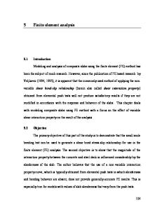
8.0E6 (Stiffness of the hook) 4.3 Output The output includes the following parameters: torque, drag, hook load, contacting nodes, translation and rotation at any node. 4.4 Sensitivity analysis of the FEA program Some input variables were selected for sensitivity analysis. They are: total length of drill string, friction coefficient, length of each element, outside diameter of drill string and the inclination angle of borehole. The output parameter is the calculated hook load. From the Figure 9, the outside diameter of the string is the most sensitive parameter, and the length of string is the second, which are obvious because the hook load is directly related to the geometry of the string, such as diameter, length, and unit weight. In fact, if we focus on those effects from non-geometrical parameters of drill string, such as inclination, element length, friction coefficient, and azimuth, the element length has the least effect in the three selected input parameters as shown in the Figure 9.

5. Verifications 5.1 Simple verification example This is a simple example of a rod that is hung and exposed to gravity (as shown in Figure 10). The rod is divided into 3 elements, so there are four nodes. The comparison between analytical model and FEA is shown in Table 1. 5.2 Vertical well drilling example This is an example in which the drill string is in a vertical well as shown in Figure 11. The drill string is hanging from a hook, and rotates with a constant speed at the well head; the bottom of the string is applied with a reactive load (WOB). With the FEA program, the hook load and displacements including rotation at any node is obtained. The known parameters: n =60 RPM ω=2πn/60=6.28(rad/s) Total elements=200 Length of the string=2000m Total weight of the string=659.73KN WOB=425KN The calculated parameters: Hook load=241.46KN Theoretical value=659.73-425=234.73 The relative error= (241.46-234.73)/234.73 =2.87% The error is accepTable ; therefore it is believed the FEA program can be used for vertical wells.

Published by Canadian Center of Science and Education

19

www.ccsenet.org/mas

Modern Applied Science

Vol. 5, No. 6; December 2011

5.3 Horizontal well drilling example This is a more complex example (azimuth=0), which is typical for horizontal well drilling. The well profile is from an actual field case. The length of the drillstring is 3351m. 5.4 Figure explanations and analysis of results Figure 12 shows the axial displacement of four nodal locations (hook, 700m, 1400m, and drill bit). It is obvious that with the increase in depth, the displacement decrease. But why is the displacement of the hook less than those at 700m and 1400m? This is because the stiffness coefficient is much larger than those at 700m and 1400m. Figure 13 shows the rotary speed at three different locations (700m, 1400m, and drill bit). The rotary speeds at different locations are different in the beginning, the speed of the drill bit response more slowly and the speed at the 700m location response the fastest. Figure 14 indicates that FEA has a closer solution under the normal condition, because it lies in the middle area of the field data region.

6. Conclusions The validity of finite element model was verified by analyzing three examples of different complicity. The values of displacement from the FEA model match those from the analytical model. The calculation of hook load is accepTable in value. The values by the FEA model agree with those from the field collected data. Acknowledgement We would like to thank NSERC, Talisman Energy and Pason Systems for supporting this research at the University of Calgary. References Aadnoy, B. S., Fazaelizadeh, M., & Hareland, G. (2010). A 3D Analytical Model for Wellbore Friction. Journal of Canadian Petroleum Technology, 49(10), 25-36. http://dx.doi.org/10.2118/141515-PA Adewuya, O. A., & Pham, S. V. (1998). A Robust Torque and Drag Analysis Approach for Well Planning and Drill string Design. Society of Petroleum Engineers, Paper SPE 39321 presented at the 1998 IADC/SPE Drilling Conference held in Dallas. Texas. 3-6 March 1998. http://dx.doi.org/10.2523/39321-MS Bueno, R. C. S., & Morooka, C. K. (1994). Analysis Method for Contact Forces Between Drillstring-Well_Riser. Society of Petroleum Engineers, Paper SPE 28723 presented at the 1994 SPE International Petroleum Conference & Exhibition of Mexico held in Veracrux. Mexico. 10-13 October 1994. http://dx.doi.org/10.2523/28723-MS Ho, H. S. (1988). An Improved Modeling Program for Computing the Torque and Drag in Directional and Deep Wells. Society of Petroleum Engineers, Paper SPE 18047 presented at the 63rd Annual Technical Conference and Exhibition of the Society of Petroleum Engineers held in Houston. TX, USA. 2-5 October 1988. http://dx.doi.org/10.2523/18047-MS Kuang, Y., Wu, Z., & Ma, D. (1999). Dynamic Simulation Model for Lateral Vibration of Cone Bits. Petroleum Machinery, 27(1), 7-9. Maehs, J., Renne, S., Logan, B., & Diaz, N. (2010). Proven Methods and Techniques to Reduce Torque and Drag in the Pre-Planning and Drilling Execution of Oil and Gas Wells. Society of Petroleum Engineers, Paper SPE 128329 presented at the 2010 IADC/SPE Drilling Conference held in New Orleans. Louisiana, USA, 2-4 February 2010. Mitchell, R. F., & Samuel, R. (2009). How Good Is the Torque/Drag Model? SPE Drilling & Completion, 62-71. SPE-105068. http://dx.doi.org/10.2523/105068-MS. Newman, K. R., & Procter, R. (2009). Analysis of Hook Load Forces During Jarring. Society of Petroleum Engineers, Paper SPE 118435 presented at the 2009 IADC/SPE Drilling Conference and Exhibition held in Amsterdam, The Netherlands. 17-19 March 2009. http://dx.doi.org/10.2118/118435-MS. Ritto, T. G., Soize, C., & Sampaio, R. (2009). Non-linear dynamics of a drill-string with uncertain model of the bit–rock interaction. International Journal of Non-Linear Mechanics, 44(2009), 865-876. http://dx.doi.org/10.1016/j.ijnonlinmec.2009.06.003 Sheppard, M. C., Wick, C., & Burgess, T. (1987). Designing Well Paths to Reduce Drag and Torque. SPE Drilling Engineering, 2(4),344-350. SPE-15463-PA. http://dx.doi.org/10.2118/15463-PA Yang, D., Rahman, M. K., & Chen, Y. (2008). Bottomhole assembly analysis by finite difference differential method. INTERNATIONAL JOURNAL FOR NUMERICAL METHODS IN ENGINEERIN. 74, 1495–1517. http://dx.doi.org/10.1002/nme.2221

20

ISSN 1913-1844

E-ISSN 1913-1852

www.ccsenet.org/mas

Modern Applied Science

Vol. 5, No. 6; December 2011

Table 1. Comparison of analytical solution with FEA Nodes

Analytical results

FEA

U1

0

0

U2

0.463835

0.453915

U3

0.742136

0.726339

U4

0.834903

0.817175

Figure 1. A 3D beam element for the drill string

Figure 2. The local and global coordinate systems

Published by Canadian Center of Science and Education

21

www.ccsenet.org/mas

Modern Applied Science

Vol. 5, No. 6; December 2011

Figure 3. Equivalent nodal forces conversion

Figure 4. Main boundaries on the drill string

Figure 5. Constraint relations between drill string and wellbore

22

ISSN 1913-1844

E-ISSN 1913-1852

www.ccsenet.org/mas

Modern Applied Science

Vol. 5, No. 6; December 2011

Figure 6. The interaction between drill string and wellbore

Figure 7. The forces applied on an element of drill string

Published by Canadian Center of Science and Education

23

www.ccsenet.org/mas

Modern Applied Science

Vol. 5, No. 6; December 2011

Figure 8. Flow chart of the FEA program

24

ISSN 1913-1844

E-ISSN 1913-1852

www.ccsenet.org/mas

Modern Applied Science

Vol. 5, No. 6; December 2011

Length of String

110%

Friction Coefficient Element Length 90%

Outside Diameter

Change Rate of Output

Inclination Angle 70%

50%

30%

10%

0%

10%

20%

30%

40%

50%

60%

-10% Change Rate of Input

Figure 9. Sensitivity analysis of some input parameters

U1 U2

U3 U4 Figure 10. FEA of a rod with one end fixed

Published by Canadian Center of Science and Education

25

www.ccsenet.org/mas

Modern Applied Science

Vol. 5, No. 6; December 2011

Figure 11. FEA of vertical well drilling

Displacements at different locations

0.35

Hook

Displacement(m)

0.3

700m 1400m

0.25

Bit 0.2 0.15 0.1 0.05 0 -0.05

1

251

501

751

1001

1251

1501

1751

Figure 12. The axial displacement of four nodal locations

26

ISSN 1913-1844

E-ISSN 1913-1852

www.ccsenet.org/mas

Modern Applied Science

Vol. 5, No. 6; December 2011

Rotary speed at different locations 10

Angular Velocity (rad/s)

8 6 700m

4

1400m

2

Bit

0 1

251

501

751

1001

1251

1501

1751

-2 Figure 13. The rotary speed at three different locations

0

1

2

Torque (klb.ft)

3

0

4

5

Field Data ( reaming & back reaming ) Analytical Model (reaming) Analytical Model (back reaming) Average Field Data

2000

Finite Element Model(Coef: 0.2)

Measured Depth (ft)

4000

6000

8000

10000

12000

Figure 14. The calculated torque versus measured depth

Published by Canadian Center of Science and Education

27