Introduction
Small T
Most-likely-path
Variational MLP
MLP solution
Numerical tests
The Variational Most-Likely-Path Jim Gatheral
Global Derivatives 2011 Paris, April 12, 2011 (Joint work with Tai-Ho Wang)
Conclusion
Introduction
Small T
Most-likely-path
Variational MLP
MLP solution
Numerical tests
Outline
Local volatility in terms of implied volatility Implied volatility in terms of local volatility Small-T approximations The most-likely-path idea The variational most-likely-path Solving for the vMLP Numerical tests with a realistic volatility surface
Conclusion
Introduction
Small T
Most-likely-path
Variational MLP
MLP solution
Numerical tests
Conclusion
Objective Given a local volatility process dS = σ` (S, t) dWt , S with σ` (S, t) depending only on the underlying level S and the time t, we want to compute implied volatilities σBS (K , T ) such that � � CBS (S, K , σBS (K , T ), T ) = E (ST − K )+ or in words, we want to efficiently compute implied volatility from local volatility. This can of course be done with numerical PDE but numerical PDE is slow, too slow for efficient calibration to implied volatilities.
Introduction
Small T
Most-likely-path
Variational MLP
MLP solution
Numerical tests
Conclusion
Motivations
The condition for no static arbitrage can be simply expressed as the non-negativity of local variance. It’s very hard in general to eliminate static arbitrage in a given parameterization of the implied volatility surface.
Knowing how to get implied volatility from local volatility helps us get accurate approximations to implied volatility in more complex models such as SABR. Efficient calibration of complex models becomes practical.
Introduction
Small T
Most-likely-path
Variational MLP
MLP solution
Numerical tests
Conclusion
Local volatility in terms of implied volatility Define the Black-Scholes implied total variance: 2 w (K , T ) := σBS (K , T ) T
In terms of the log-strike k := log K /F and the local variance v` := σ`2 (K , T ), the Dupire equation becomes v` ∂C = ∂T 2
�
∂2C ∂C − 2 ∂k ∂k
�
Then, by taking derivatives of the Black-Scholes formula and simplifying, we obtain equation (1.10) in [The Volatility Surface]: v` =
1−
� ∂w 2
k 2 w ∂k
−
1 4
∂w ∂T � 1 1 + 4 w
� ∂w 2 ∂k
+
1 ∂2w 2 ∂k 2
(1)
Introduction
Small T
Most-likely-path
Variational MLP
MLP solution
Numerical tests
Special Case: No Skew If the skew
∂w ∂k
is zero, (1) reduces to v` =
∂w ∂T
In this special case, the local variance reduces to the forward Black-Scholes implied variance. The solution is of course Z w (T ) =
T
v` (t) dt 0
or equivalently in the suggestive form, 2 σBS (T ) =
1 T
Z 0
T
σ`2 (t) dt =
Z 0
1
σ`2 (α T ) dα.
Conclusion
Introduction
Small T
Most-likely-path
Variational MLP
MLP solution
Numerical tests
Conclusion
Inverting the equation
We have a formula (1) for getting local volatility from implied. All we need to do is to invert this formula! This is certainly not easy and has not so far proved to be possible in closed-form.
In the limit of small time however, equation (1) can been solved.
Introduction
Small T
Most-likely-path
Variational MLP
MLP solution
Numerical tests
Conclusion
The BBF approximation Recall equation (1) for local variance in terms of implied: v` =
1−
� k ∂w 2 2 w ∂k
−
1 4
∂w ∂T � 1 1 4 + w
� ∂w 2 ∂k
+
1 ∂2w 2 ∂k 2
Noting that w ∼ O(T ), in the limit of small T , to leading order in T we may write v` ≈
1−
∂w ∂T � k ∂w 2 2 w ∂k
Further supposing that to lowest order in T , w ≈ σBS (k, 0)2 T and making the change of variable u=
1 , σBS (k, 0)
(2)
Introduction
Small T
Most-likely-path
Variational MLP
MLP solution
Numerical tests
Conclusion
we may rewrite (2) as 1 u2 � ∂u 2 + ku ∂k
σ(k, 0)2 ≈ 1 or rearranging
∂ 1 (k u) = ∂k σ(k, 0) giving us the BBF approximation of [Berestycki, Busca and Florent]: 1 1 1 ≈ := σBS (K , T ) σ0 (k) ln K /S0
Z
K
S0
dS = S σ(S, 0)
Z 0
1
dα σ(α k, 0)
Introduction
Small T
Most-likely-path
Variational MLP
MLP solution
Numerical tests
First order term [Henry-Labord`ere] expands σBS (·) as σBS (k, T ) = σ0 (k) + σ1 (k) T + O(T 2 ). Substituting into (1) and matching powers of T , he obtains the first order correction: ( p σ(0, 0) σ(k, 0) σ0 (k)3 σ1 (k) = ln k2 σ0 (k) � �2 ) Z k y ∂t σ(y , t)|t=0 ∂ dy − σ(y , 0) ∂y σ0 (y ) 0 where σ0 (k) is the lowest-order (BBF) approximation derived earlier.
Conclusion
Introduction
Small T
Most-likely-path
Variational MLP
MLP solution
Numerical tests
Heat kernel expansion
In [GHLOW], we compute implied volatility for short times using the heat kernel expansion up to second order. σBS (k, T ) ≈ σ0 (k) + σ1 (k) T + σ2 (k) T 2 The first two terms, σ0 and σ1 agree with BBF and H-L respectively. σ2 is somewhat too complicated to reproduce here!
Conclusion
Introduction
Small T
Most-likely-path
Variational MLP
MLP solution
Numerical tests
Conclusion
Call price in terms of the transition density
Let p(t, s; t 0 , s 0 ) be the transition probability density. Then � � C (s, t, K , T ) = E (ST − K )+ |St = s Z = (s 0 − K )+ p(t, s; T , s 0 )ds 0 As a function of t and s, p satisfies the backward Kolmogorov equation: 1 Lp := pt + s 2 σ`2 (s, t) pss = 0, 2 Subindices refer to respective partial derivatives.
(3)
Introduction
Small T
Most-likely-path
Variational MLP
MLP solution
Numerical tests
Heat kernel expansion Heat kernel expansion for transition density p(t, s; t 0 , s 0 ) when t 0 − t is small: e
−
d 2 (s,s 0 ,t) 2(t 0 −t)
p(t, s; t 0 , s 0 ) ∼ p 2π(t 0 − t)s 0 σ` (s 0 , t 0 )
n X
Hk (t, s, s 0 )(t 0 − t)k
k=0
R 0 s 0 d(s, s 0 , t) = s ξσ`dξ (ξ,t) : geodesic distance between s to s q hR 0 i s dt (η,s 0 ,t) ` (s,t) H0 (t, s, s 0 ) = ssσ exp dη 0 σ (s 0 ,t) s ησ` (η,t) ` R i−1 0 (η,s 0 ,t)LHi−1 (t,s,s ) s d Hi (t, s, s 0 ) = Hd 0i (s,s 0 ,t) s 0 H0 (η,s 0 ,t)a(η,t) dη
Conclusion
Introduction
Small T
Most-likely-path
Variational MLP
MLP solution
Numerical tests
Conclusion
Heat kernel expansion for Black-Scholes Heat kernel expansion for Black-Scholes transition density pBS (t, s; t 0 , s 0 ) when t 0 − t is small: 0
0
pBS (t − t, s, s ) = p R 0 s dBS (s, s 0 ) = s
e
−
2 (s,s 0 ) dBS 2(t 0 −t)
r
2π(t 0 − t) σBS s 0
dξ σBS ξ
=
1 σBS
� 2 0 �k ∞ (t − t) s X (−1)k σBS s0 k! 8 k=0
0 log ss
The lowest order heat kernel coefficient is given by r s BS 0 H0 (t, s, s ) = . s0
Introduction
Small T
Most-likely-path
Variational MLP
MLP solution
Numerical tests
Conclusion
The heat-kernel expansion of implied volatility Implied volatility σBS is defined as the unique solution to C (s, t, K , T ) = CBS (s, t, K , T , σBS )
Substitute the heat kernel approximation to the transition density p(·) into the expression for both the model price C and the Black-Scholes price CBS . Expand both sides of (4) in powers of T − t. On the RHS, also expand the BS implied volatility: σBS (K , T ) ≈ σBS,0 + σBS,1 (T − t) + σBS,2 (T − t)2 Match the coefficients of powers of T − t.
(4)
Introduction
Small T
Most-likely-path
Variational MLP
MLP solution
Numerical tests
Conclusion
What’s wrong with small-time expansions? Small-time expansions like that of [GHLOW] use only information about the volatility surface in a neighborhood of the origin (the at-the-money, zero time to expiration point). Shouldn’t an implied volatility approximation take into account all of the local volatility surface? Information from the neighborhood of the origin does generate accurate implied volatility estimates for time-homogeneous models such as CEV. This cannot be the case for empirically reasonable local volatility surfaces. For empirically reasonable local volatility surfaces, the k and t derivatives may not even exist at the origin in which case the short-time expansions presented earlier cannot be performed.
Introduction
Small T
Most-likely-path
Variational MLP
MLP solution
Numerical tests
Conclusion
Integral representation of implied volatility
Alternatively, we have integral representations of implied volatility such as the one presented in [The Volatility Surface]: � � Z 1 T E σt2 St2 ΓBS (St ) 2 2 � � dt (5) σBS (K , T ) = σ ¯ (0) = T 0 E St2 ΓBS (St ) which expresses implied variance as the time-integral of expected instantaneous variance σt2 under some probability measure. Note that equation (5) is circular because the gamma ΓBS (St ) of the option on the rhs depends on σBS (K , T ) on the lhs.
Introduction
Small T
Most-likely-path
Variational MLP
MLP solution
Special case: Black-Scholes
Suppose σt = σ(t), a function of t only. Then � � E σ(t)2 St2 ΓBS (St ) � � = σ(t)2 E St2 ΓBS (St ) and from (5), 1 σBS (K , T ) = T 2
Z
T
σ 2 (t) dt
0
which has no dependence on the strike K .
Numerical tests
Conclusion
Introduction
Small T
Most-likely-path
Variational MLP
MLP solution
Numerical tests
Conclusion
Visualizing implied volatility Equation (5) may be rewritten in the form 2 σBS (K , T ) =
1 T
Z TZ
q(St ; S0 , K , T ) σ`2 (St , t) dSt dt
0
where q (St , t; S0 , K , T ) :=
p(0, s0 ; St , t)St2 ΓBS (St ) � � E St2 ΓBS (St )
� � and σ`2 (St , t) = EP σt2 |St is the local variance or alternatively in terms of xt := log (St /F ): 2 σBS (K , T )
1 = T
Z TZ 0
q(xt , t; xT , T )σ`2 (xt , t)dxt dt
(6)
Introduction
Small T
Most-likely-path
Variational MLP
MLP solution
Numerical tests
Conclusion
The most-likely-path
15 1 10 5 0 1 0.8 -0.4 .4
0.6 -0.2
0.4 0 0.2
0.2 0.4
2 σBS (K , T ) =
≈
Z Z 1 T q(xt , t; xT , T ) σ`2 (xt , t)dxt dt T 0 Z 1 T 2 σ` (˜ xt , t)dt T 0
where x˜t is the most likely path.
(7)
Introduction
Small T
Most-likely-path
Variational MLP
MLP solution
Numerical tests
Conclusion
The most-likely-path formula in words
Equation (7) says that the Black-Scholes implied variance of an option with strike K is given approximately by the integral from valuation date (t = 0) to the expiration date (t = T ) of the local variances along the most-likely-path. Implied volatility is root-mean-squared local volatility.
However, not only is it not trivial to compute the path x˜t but there is no unique definition of x˜t . [The Volatility Surface] chooses x˜t as the path that maximizes the density q(xt , t; xT , T ). [Reghai] chooses x˜t to be the conditional expectation of xt wrt q(·).
Introduction
Small T
Most-likely-path
Variational MLP
MLP solution
Numerical tests
Conclusion
The main idea: Heat kernel + Chapman Kolmogorov
We have highly accurate approximations for small T . We want to take information about the entire local volatility surface into account. Use the heat kernel approximation to approximate the transition density for a small timestep T /n and apply Chapman-Kolmogorov to get an approximation to the density over a large timestep. Use the Laplace asymptotic formula to approximate the resulting n-dimensional integral.
Introduction
Small T
Most-likely-path
Variational MLP
MLP solution
Numerical tests
Laplace asymptotic formula
Asymptotic expansion of the integral as τ → 0+ Z ∞ φ(x) φ(x ∗ ) f 0 (x ∗ ) e − τ f (x)dx ∼ τ 2 e − τ [φ0 (x ∗ )]2 0 Assumptions: f is identically zero when 0 ≤ x ≤ x ∗ . φ is increasing in [x ∗ , ∞).
Conclusion
Introduction
Small T
Most-likely-path
Variational MLP
MLP solution
Numerical tests
Conclusion
Example: Approximation to the price of a call Let τ = T − t. Then Z C (s, t, K , T ) =
∞
(s − K )+ p(t, s; T , s 0 )ds 0
0
≈ =
d 2 (s,s 0 ,t) Z ∞ − 2τ 1 0 + e √ (s − K ) 0 H0 (t, s, s 0 )ds 0 s σ(s 0 , T ) 2πτ 0 Z ∞ d 2 (s,s 0 ,t) 1 √ e − 2τ G0 (t, s, T , s 0 )ds 0 (8) 2πτ K
where G0 (t, s, T , s 0 ) = (s 0 − K )
H0 (t, s, s 0 ) s 0 σ(s 0 , T )
Introduction
Small T
Most-likely-path
Variational MLP
MLP solution
Numerical tests
Conclusion
Approximations to the call price Assuming s < K and performing the integration in (8), we obtain 3
d2 G00 τ2 . C (s, t, K , T ) ≈ √ e − 2τ (dd 0 )2 2π
d = d(s, K , t) and d 0 = G00 =
∂G0 ∂s 0 (t, s, T , K )
=
∂d ∂s 0 (s, K , t) H0 (t,s,K ) K σ` (K ,T )
In the special case of Black-Scholes (with k = log K /s), we get CBS (s, t, K , T , σBS ) ≈
√
3
2
τ 2 − k2 σ 3 s K √ e 2σBS τ BS . k2 2π
Introduction
Small T
Most-likely-path
Variational MLP
MLP solution
Numerical tests
Chapman Kolmogorov Let s = (s0 , · · · , sn ) and t = (t0 , · · · , tn ). By Chapman-Kolmogorov we have p(s0 , t0 ; sn , tn ) =
Z Y n
p(sk−1 , tk−1 ; sk , tk )ds.
k=1
The option price then becomes an n dimensional integration Z
+
E[(ST − K ) ] =
+
(sn − K )
n Y
p(ti−1 , si−1 ; ti , si )ds
i=1
Z (sn − K )
= sn ≥K
n Y i=1
p(ti−1 , si−1 ; ti , si )ds
Conclusion
Introduction
Small T
Most-likely-path
Variational MLP
MLP solution
Numerical tests
Recap of steps in derivation of MLP
+
Z
E[(ST − K ) ] =
(sn − K ) sn ≥K
n Y
p(ti−1 , si−1 ; ti , si )ds
i=1
Express the transition density as a convolution of transition densities over small time intervals using Chapman-Kolmogorov. Approximate transition density by the heat kernel expansion over each small time interval. Approximate the resulting n-dimensional integral using the Laplace asymptotic formula. Push n to infinity.
Conclusion
Introduction
Small T
Most-likely-path
Variational MLP
MLP solution
Numerical tests
Heat kernel expansion again
Heat kernel expansion for transition density p(t, s; t 0 , s 0 ) when t 0 − t is small: p(t, s; t 0 , s 0 ) ∼ e
R 0 s d(s, s 0 , t) = s
−
d 2 (s,s 0 ,t) 2(t 0 −t)
dξ ξσ(ξ,t) :
H(t, s; t 0 , s 0 ) p 2π(t 0 − t)s 0 σ(s 0 , t 0 )
geodesic distance between s to s 0
H: series expansion of heat kernel coefficients
Conclusion
Introduction
Small T
Most-likely-path
Variational MLP
MLP solution
Numerical tests
Conclusion
Laplace type integral Approximating the transition density using the heat kernel expansion, we end up with a Laplace type integral. Heat kernel expansion for product of transition densities n Y
p(ti−1 , si−1 ; ti , si ) ∼ e
i=1
where Dn (s, t) =
n X
−
Dn (s,t) 2∆t
n Y H(ti−1 , si−1 ; ti , si ) √ , 2π∆tsi σ(si , ti ) i=1
d 2 (si−1 , si , ti−1 ).
i=1
Laplace type integral Z n Dn (s,t) Y H(ti−1 , si−1 ; ti , si ) √ E[(ST − K )+ ] ≈ (sn − K ) e − 2∆t ds 2π∆ts σ(s , t ) sn ≥K i i i i=1
Introduction
Small T
Most-likely-path
Variational MLP
MLP solution
Numerical tests
Minimization problem for discrete-time MLP
As ∆t → 0+ , the main contribution of the Laplace type integral comes from the solution of the minimization problem: min s
subject to sn = K .
n 1 X 2 d (si−1 , si , ti−1 ) 2∆t i=1
Conclusion
Introduction
Small T
Most-likely-path
Variational MLP
MLP solution
Numerical tests
Conclusion
Continuous-time limit
Since
∆si , d(si−1 , si , ti−1 ) ≈ a(si−1 , ti−1 )
we have 2 n ∆si 1 X ∆t lim ∆t a(si−1 , ti−1 ) ∆t→0 2 k=1 Z T s˙ (t) 2 1 dt = 2 0 a(s(t), t)
n 1 X 2 lim d (si−1 , si , ti−1 ) = ∆t→0 2∆t i=1
Introduction
Small T
Most-likely-path
Variational MLP
MLP solution
Numerical tests
Conclusion
The variational most-likely-path
In the limit as ∆t approaches zero, the minimization problem becomes the following variational problem 1 min s(t) 2
Z 0
T
�
s˙ (t) a(s(t), t)
�2 dt
(9)
subject to s(0) = s0
and
s(T ) = K .
(10)
We call the solution to (9):(10), the variational most-likely-path (vMLP).
Introduction
Small T
Most-likely-path
Variational MLP
MLP solution
Numerical tests
Conclusion
The Euler-Lagrange equation
The variational most-likely-path (vMLP) for a European option thus solves the Euler-Lagrange equation for the variational problem (9):(10) which can be written as � � d s˙ ∂t a s˙ = (11) dt a a a with initial and terminal conditions s(0) = s0 ,
s(T ) = K .
Introduction
Small T
Most-likely-path
Variational MLP
MLP solution
Numerical tests
Conclusion
Matching with Black-Scholes Once the vMLP s ∗ (t) is obtained, the call price is approximately C (s0 , K , T ) ∼ e
− 21
RTh 0
i2 s˙ ∗ (t) dt a(s ∗ (t),t)
.
Recall the call price approximation under Black-Scholes: CBS (s, t, K , T , σBS ) ≈
√
3
2
τ 2 − k2 σ 3 s K √ e 2σBS τ BS . k2 2π
By matching exponents to leading order, we obtain Implied volatility at lowest order �2 Z T� 1 1 s˙ ∗ (t) = dt 2 |k| 0 a(s ∗ (t), t) σBS,0 T
(12)
Introduction
Small T
Most-likely-path
Variational MLP
MLP solution
Numerical tests
Conclusion
Solution of the variational problem With the change of variables x(t) := log s(t)/s0 ;
a(s(t), t) = s(t) σ(x(t), t),
the Euler-Lagrange equation (11) becomes � � �� d x(t) ˙ log = ∂t log σ(x, t)|x=x(t) =: f (x(t), t) (13) dt σ(x(t), t) with boundary conditions x(0) = 0, x(T ) = k. Note that for any given closed-form parameterization of the local volatility surface, f (·) is known in closed-form. f (·) is a measure of the time-inhomogeneity of the local volatility surface. In particular, if the local volatility function is time-independent, f (·) = 0.
Introduction
Small T
Most-likely-path
Variational MLP
MLP solution
Numerical tests
Conclusion
A recursive expression for the vMLP
Integrating (13) twice, we obtain �R u Rt 0 du σ(x(u), u) exp 0 f (x(s), s) ds x(t) = k R T �R u . 0 du σ(x(u), u) exp 0 f (x(s), s) ds
(14)
Equation (14) leads to an efficient fixed-point algorithm for finding the vMLP reminiscent of [Reghai]. The natural choice of first guess is just the straight line x0 (t) = k t/T . Note that the vMLP for k = 0 (K = s0 ) is x(t) = 0.
Introduction
Small T
Most-likely-path
Variational MLP
MLP solution
Numerical tests
Conclusion
Implied volatility in terms of local volatility
In terms of the local volatility σ(x, t), equation (12) may be rewritten as Implied volatility in terms of local volatility nR o RT t 1 σ(x(t), t) exp f (x(s), s) ds dt T 0 0 r σBS,0 = n o RT Rt 1 T 0 exp 2 0 f (x(s), s) ds dt
(15)
Introduction
Small T
Most-likely-path
Variational MLP
MLP solution
Numerical tests
Conclusion
Time-separable local volatility
Suppose σ(x, t) = σ(x) θ(t) for some functions σ(·) and θ(·). Then by the definition of f (·), f (x, t) = With φ(x) =
Rx
dξ 0 σ(ξ) ,
θ0 (t) . θ(t)
the solution for the vMLP is
x(t) = φ
−1
Rt φ(k)
R 0T 0
θ2 (s) ds θ2 (s) ds
! .
(16)
Introduction
Small T
Most-likely-path
Variational MLP
MLP solution
Numerical tests
Conclusion
Time-separable local volatility
Equation (15) then becomes Implied volatility in a time-separable local volatility model RT 1 T 0 σ(x(t)) θ(t) dt σBS,0 = q R T 2 1 T 0 θ (t) dt
(17)
Introduction
Small T
Most-likely-path
Variational MLP
MLP solution
Numerical tests
Conclusion
Time-homogeneous local volatility
If σ(x, t) = σ(x) is time-homogeneous, θ(·) is constant, and σBS,0
1 = T
Z
T
σ(x(t)) dt.
(18)
0
At first sight, (18) seems to differ from the BBF formula. In (18), implied volatility is expressed as an arithmetic mean and in the BBF formula as a harmonic mean.
We show in [Gatheral and Wang] that the two expressions are in fact equivalent.
Introduction
Small T
Most-likely-path
Variational MLP
MLP solution
Numerical tests
Conclusion
Time-changed time-homogenous local volatility
The time-separable case can be reduced to the time-homogeneous case by the simple deterministic time-change Z t θ2 (s) ds. τ (t) = 0
We show that the vMLP (16) in the time-separable case is just the time-changed version of the vMLP in the time-homogeneous case.
Introduction
Small T
Most-likely-path
Variational MLP
MLP solution
Numerical tests
Conclusion
Accuracy of our implied volatility approximation
Thus our approximation (15) behaves correctly under a deterministic time-change. It follows that the numerical accuracy of our approximation must be just as great in the time-separable case as it is in the time-homogeneous case. We know that the BBF formula is typically highly accurate in the time-homogeneous case. It follows that (15) is also typically highly accurate in the time-separable case. No point in repeating the time-separable numerical examples in [GHLOW]!
Introduction
Small T
Most-likely-path
Variational MLP
MLP solution
Numerical tests
Conclusion
Accuracy of our implied volatility approximation
We have just established that our new approximation is highly accurate in the case of time-separable local volatility. This motivates us to test our new formula with a local volatility function that is both much more realistic and more difficult. Difficult in the sense that its derivatives at t = 0 do not exist. In particular, small-time expansions are not possible.
Introduction
Small T
Most-likely-path
Variational MLP
MLP solution
Numerical tests
Conclusion
Figure 3.2: 3D plot of volatility surface Here’s a 3D plot of the volatility surface as of September 15, 2005:
Implied vol. n
tio
t
ra pi
Ex Log
−str ik
ek
k := log K /F is the log-strike and t is time to expiry.
Introduction
Small T
Most-likely-path
Variational MLP
MLP solution
Numerical tests
Conclusion
3D plot of approximate local volatility surface
Local variance
n
Log
ir
io at
-strik
ek
p Ex
t
Introduction
Small T
Most-likely-path
Variational MLP
MLP solution
Numerical tests
Local volatility surface parameterization � s� �2 � k k √ − m + σ2 t σ 2 (k, t) = a + b ρ √ − m + t t with a = 0.0012 b = 0.1634 σ = 0.1029 ρ = −0.5555 m = 0.0439 Each slice is SVI.
Conclusion
Introduction
Small T
Most-likely-path
Variational MLP
MLP solution
Numerical tests
Picture for the sceptical
-0.3
-0.2
-0.1 Log-Strike
0.0
0.1
0.4 0.0
0.1
Implied Vol. 0.2 0.3
0.4 Implied Vol. 0.2 0.3 0.1 0.0
0.0
0.1
Implied Vol. 0.2 0.3
0.4
0.5
T = 0.50
0.5
T = 0.25
0.5
T = 0.18
-0.5 -0.4 -0.3 -0.2 -0.1 Log-Strike
0.0
0.1
-0.4 -0.2 Log-Strike
0.0
0.2
-0.2 Log-Strike
0.0
0.5 0.0
0.1
Implied Vol. 0.2 0.3
0.4
0.5 0.4 0.1 0.0 -0.6
-0.4
T = 1.75
Implied Vol. 0.2 0.3
0.4 Implied Vol. 0.2 0.3 0.1 0.0 -0.8
-0.6
T = 1.25
0.5
T = 0.75
-0.6
-0.4 -0.2 Log-Strike
0.0
0.2
-0.6
-0.4
-0.2 Log-Strike
0.0
0.2
Orange lines are from PDE computations, red and blue triangles are bid and offered vols respectively. Fits are not too bad!
Conclusion
Introduction
Small T
Most-likely-path
Variational MLP
MLP solution
Numerical tests
Numerical tests In the following slide, we compare various implied volatility approximations with an accurate estimate from numerical PDE: The brown solid lines are from PDE computations The red dotted lines are the vMLP estimates σBS,0 The orange dash-dotted lines are from Adil Reghai’s fixed point algorithm The green dashed lines correspond to a na¨ıve extension (BBFe) of the BBF formula: 1 ≈ σBS (k, T )
Z 0
1
dα σ` (α k, α T )
Expirations shown are actual SPX market expirations as of September 15, 2005.
Conclusion
Introduction
Small T
Most-likely-path
Variational MLP
MLP solution
Numerical tests
Comparison of approximations
1.5
2.0
0.5 0.4 0.3 0.1 0.0 0.5
1.0
1.5
2.0
0.5
1.0
1.5 Strike
T= 0.501
T= 0.75
T= 1.25
1.5 Strike
2.0
0.4 0.3 0.0
0.1
0.2
Implied volatility
0.4 0.3 0.0
0.1
0.2
Implied volatility
0.4 0.3 0.2 0.1
1.0
2.0
0.5
Strike
0.5
Strike
0.0 0.5
0.2
Implied volatility
0.4 0.3 0.0
0.1
0.2
Implied volatility
0.4 0.3 0.2
Implied volatility
0.1 0.0
1.0
0.5
0.5
Implied volatility
T= 0.252
0.5
T= 0.175
0.5
T= 0.0986
0.5
1.0
1.5 Strike
2.0
0.5
1.0
1.5 Strike
2.0
Conclusion
Introduction
Small T
Most-likely-path
Variational MLP
MLP solution
Numerical tests
Longer-dated smiles
1.5
2.0
0.30 0.25 0.20
Implied volatility
0.10 0.5
1.0
1.5
2.0
0.5
1.0 Strike
T= 8
T= 10
T= 12
1.5 Strike
2.0
2.0
1.5
2.0
0.25 0.20
Implied volatility
0.10
0.15
0.25 0.20
Implied volatility
0.10
0.15
0.25 0.20 0.15
1.0
1.5
0.30
Strike
0.30
Strike
0.10 0.5
0.15
0.25 0.20
Implied volatility
0.10
0.15
0.25 0.20
Implied volatility
0.15 0.10
1.0
0.30
0.5
Implied volatility
T= 6
0.30
T= 4
0.30
T= 2
0.5
1.0
1.5 Strike
2.0
0.5
1.0 Strike
Conclusion
Introduction
Small T
Most-likely-path
Variational MLP
MLP solution
Numerical tests
Zoomed view of short expiration smile
0.3 0.2 0.1 0.0
Implied volatility
0.4
0.5
T= 0.175
0.5
1.0
1.5 Strike
2.0
Conclusion
Introduction
Small T
Most-likely-path
Variational MLP
MLP solution
Numerical tests
Zoomed view of long-dated smile
0.20 0.15 0.10
Implied volatility
0.25
0.30
T= 12
0.5
1.0
1.5 Strike
2.0
Conclusion
Introduction
Small T
Most-likely-path
Variational MLP
MLP solution
Numerical tests
Observations
Our vMLP approximation dominates the alternative most-likely-path approximations We note that BBFe does better than Reghai for shorter expirations and Reghai does better than BBFe for longer expirations Variational MLP does better than either!
Conclusion
Introduction
Small T
Most-likely-path
Variational MLP
MLP solution
Numerical tests
Conclusion
Convexity error For all three most-likely-path approximations, there is consistently a large approximation error at the cusp of the smile. As noted in [Guyon and Henry-Labord`ere], this is because the most-likely-path technique fails when there is substantial curvature in the local volatility function. A convexity correction is required. Fixing a time t, one cannot reasonably approximate an integration over all possible prices of the underlying xt by one point, the most-likely point x˜(t).
The price to be paid for improved accuracy is in computational effort; a brute-force numerical PDE computation may be faster (and more accurate). In contrast, our fixed-point vMLP algorithm is very fast, typically converging within 3 or 4 iterations.
Introduction
Small T
Most-likely-path
Variational MLP
MLP solution
Numerical tests
Conclusion
Summary and conclusion We have derived a new most-likely-path estimate which we call variational MLP for approximating the implied volatility surface given a local volatility function. The vMLP estimate is a natural extension of the BBF formula that behaves correctly under a deterministic time-change, in contrast to prior choices of most-likely-path. Our numerical tests indicate that the vMLP estimate outperforms two competing definitions of most-likely-path: a popular definition due to Adil Reghai and a na¨ıve extension of the BBF formula. How to improve the accuracy of our variational MLP estimate by for example better approximating the integration over xt is left for future research.
Introduction
Small T
Most-likely-path
Variational MLP
MLP solution
Numerical tests
References [Berestycki, Busca and Florent] Henri Berestycki, J´ erˆ ome Busca, and Igor Florent Computing the implied volatility in stochastic volatility models Communications on Pure and Applied Mathematics 57 1–22 (2004). [Gatheral] Jim Gatheral. The Volatility Surface: A Practitioner’s Guide. John Wiley and Sons, Hoboken, NJ, 2006. [GHLOW] Jim Gatheral, Elton P Hsu, Peter Laurence, Cheng Ouyang, and Tai-Ho Wang Asymptotics of implied volatility in local volatility models Mathematical Finance Forthcoming (2011). [Gatheral and Wang] Jim Gatheral and Tai-Ho Wang The heat-kernel most-likely-path approximation http://papers.ssrn.com/sol3/papers.cfm?abstract_id=1663318 (2010). [Guyon and Henry-Labord` ere] Julien Guyon and Pierre Henry-Labord` ere From local to implied volatilities http://papers.ssrn.com/sol3/papers.cfm?abstract_id=1663878 (2010). [Henry-Labord` ere] Pierre Henry-Labord` ere, Analysis, Geometry, and Modeling in Finance: Advanced Methods in Option Pricing. CRC Press, 2009. [Reghai] Adil Reghai The hybrid most likely path Risk Magazine, April 2006.
Conclusion