J. Serv. Sci. & Management, 2008,1: 172-192 Published Online August 2008 in SciRes (www.SRPublishing.org/journal/jssm)

The Theory of the Revenue Maximizing Firm Beniamino Moro Department of Economics, University of Cagliari, Viale Sant’Ignazio 17 - 09123 Cagliari (Italy) Email: [email protected]

ABSTRACT An endogenous growth model of the revenue maximizing firm is here presented. It is demonstrated that, in a static analysis, a revenue maximizing firm in equilibrium equates the average product of labor to the wage rate. In a dynamic analysis, the maximization rule becomes the balance between the rate of marginal substitution - between labor and capital - and the ratio of the wage rate over the discount rate. When the firm satisfies this rule, it grows endogenously at the rate of return on capital. The firm may also have multiple stationary equilibria, which are very similar to the static equilibrium. JEL classification: D21, O41.

Keywords: firm, theory of the firm, revenue maximization, endogenous growth

1. Revenue Maximization Versus Profit Maximization and the Theory of the Firm The original idea of a firm that maximizes revenue instead of profit was put forward by Baumol [2, 3], and further investigated during the sixties by Cyert-March [12], Galbraith [19], Winter [39] and Williamson [36]. Autonomously, a similar idea was also investigated by Rothbard [31], a precursor of the Austrian theory of the firm.1 Nonetheless, the main stream economic thought, as Cyert-Hedrick [11] pointed out in their review article, remains characterized by an ideal market with firms for which profit maximization is the single determinant of behavior. 2 Indeed, the relevance of pure profitmaximization is not so obvious for modern corporations when ownership and control of the firm are separated and there are no dominant owners that merely maximize their profits [27]. 1

See Anderson [1], and for the Austrian school see Foss [15, 18], and Witt [41]. 2 In fact, during the ‘30s and ‘40s, a great dispute was due to the “Old Marginalist Debate” which questioned the relevance of the profitmaximization assumption in neoclassical theory of the firm. In the ‘70s, the marginalist debate changed tone with the emergence of the theories of agency costs, property rights, and transactions costs theories of the firm. These gave rise to the “New Institutionalist” field of research, where the object of study changed from how to reconcile firm behavior with marginalist principles to how to reconcile firm structure with marginalist principles. Following the seminal work by Coase [8], papers belonging to the Institutionalist debate can be divided in the transactions costs economics [24, 37, 38], and the contractual field of research [6, 13, 21, 22]. The old marginalist debate re-emerged in the ‘80s with the evolutionary theory of the firm by Nelson-Winter [30], Winter [40], and Foss [14]. Finally and more recently, we also have a “Knowledgebased” theory of the firm [16, 17, 20], and a “Resource-based” theory [9, 10].

Copyright © 2008 SciRes

More recently, the revenue-maximization dominance hypothesis has been re-proposed by Uekusa-Caves [34], Komiya [25, 26], Blinder [4, 5] and Tabeta-Wang [32, 33]. In all these papers it is argued that the separation of ownership and control in public companies causes a deviation of management from the pure profit maximization principle and provides a considerable degree of decisionmaking autonomy for managers. In fact, in an oligopolistic market, each firm may set up its own goal, and the choice to maximize revenue or profit depends on the real interests of the managers, and is also influenced by the corporate culture and institutional arrangements of the country where the firm operates. According to Kagono et al. [23], the principal objectives of Japanese firms are growth and market-share gaining, which imply that they are revenue maximizers, while US corporations emphasize more on short run investment returns and capital gains, which means that they are profit maximizers.3 In 3

Blinder [5] builds up a model to demonstrate that revenue-maximizers like Japanese firms have an advantage when competing with profitmaximizers. Particularly, he points out that the revenue-maximizer is likely to drive its profit-maximizers rivals out of business if either average costs are declining or learning is a positive function of cumulative output. Tabeta-Wang [33] find the following four reasons to explain why Japanese firms are in general able to act like revenue-maximizers. First of all, in Japan, expansion in firm-size is a necessary condition to maintain the life-time employment system and internal promotion. Secondly, a faster growth of the firm helps hiring new young employees, and keeping low the average age of the work force helps to maintain low labor costs. Thirdly, Japanese firms pursue the growth-oriented strategy also because there is little external pressure for short-term earnings, and tax rates on reinvested earnings are lower than tax rates on dividends.

JSSM

The Theory of the Revenue Maximizing Firm fact, as Anderson [1] points out, the profit maximizing versus the revenue maximizing strategy of the firm still stays as an open question, the answer to which only time will tell. A parallel problem to this dispute is how to formalize the firm behavior in the two cases. At this regard, the mainstream microeconomic analysis has been mainly oriented to the profit maximization strategy, while very little attention has been devoted to the revenue maximizing case. Apart from the static analysis during the sixties, the latter field of research is very poor. After the seminal work by Leland [28], Van Hilton-Kort-Van Loon [35] and Chiang [7] put the problem in the contest of the optimal control theory and demonstrated that a revenue maximizing firm subject to a minimum profitability constraint is in equilibrium at a smaller capital-labor ratio than a profit maximizing one. This result is also obtained here. Anyway, Leland’s model suffers of some limitations - e.g. he considers constant the share of profits used to self-financing the accumulation of capital - which preclude him to develop a complete dynamic model which fully describes the dynamics of a revenue maximizing firm. The aim of this paper is to fill the gap in this field of research, presenting a complete endogenous growth model of a revenue maximizing firm. The paper is organized as follows. In section 2, the problem of a revenue maximizing firm versus the classical problem of profit maximization is analyzed from a static point of view. First of all, the analysis is made without taking into account a minimum acceptable return on capital constraint (section 2.1) and then with such a constraint (section 2.2). In section 2.3, the analysis is generalized into a rate of profit maximization problem and into a revenue per unit of capital maximization problem, respectively. We obtain the fundamental rule followed by a static revenue maximizing firm, according to which the firm equates the average product of labor to the wage rate. The same rule also applies in a dynamic context. In section 3, we use the optimal control theory to describe the dynamics of a revenue maximizing firm. With respect to Leland’s model, this paper differs on the following two assumptions: a) we suppose that the firm’s accumulation of capital is limited to the non distributed profits and b) we also suppose that the share of the reinvested profits is endogenously determined by the firm, while in Leland’s model this is a constant. We also demonstrate that only some of the possible dynamic equilibria (stationary equilibria) correspond to those discussed in the static analysis. Anyway, it is also demonstrated that an endogenous growth equilibrium of the firm does exist, Lastly, there is some possibility that administrative guidance and controls lead Japanese firms to act like revenue-maximizers. At this regard, Nakamura [29] clamed that administrative guidance and controls play a role as a “shelter from the storm” once the firm grows beyond the limits of a market accepted profitability.

Copyright © 2008 SciRes

173

where the rate of growth is obtained from the solution of a system of differential equations which fully describes the dynamics of the model. Also in this section, the problem is first analyzed without taking into account any minimum acceptable return on capital constraint (sections 3.1-3.4) and then with such a constraint (section 3.5). Our main conclusion is that, in a dynamic context, the equilibrium of a revenue maximizing firm requires not only that the marginal rate of substitution between labor and capital to be equal to the shadow value of the capital-labor ratio, but that this value also balances the ratio of the wage rate over the discount rate. Further, if we introduce a minimum acceptable return on capital constraint, this must be added to the discount rate when determining the equilibrium equality with the rate of marginal substitution between labor and capital. As a consequence, a change of the minimum acceptable return on capital rate has the same effect as a variation of the discount rate. Finally, section 4 is devoted to the concluding remarks.

2. The Static Analysis of the Firm Behavior 2.1. The Equilibrium Conditions Without a Minimum Acceptable Return on Capital Constraint We make the following neoclassical assumptions on the firm production function Q=Q(K, L), where K is capital and L is labor: a) Q is linear homogenous and strictly quasi-concave, which implies that Q=Q(K, L)=Lf(k), where f(k)=Q(K/L, 1) and k=K/L; f(0)=0 and lim f ( k ) = ∞ ; k →∞

b) the marginal productivity of capital QK = f '(k ) has lim f ' (k ) = ∞ and lim f ' (k ) = 0 ;

k →0

k →∞

c) the marginal productivity of labor QL = f (k ) − kf ' (k ) has lim = 0 and lim = ∞. k →0

k →∞

We also assume that the price of the firm’s output is normalized to one, so that both the nominal and the real wage rate can be indicated by w. First of all, we demonstrate that if the firm program is: Maximize [Q( K , L) − wL ]

(1)

subject to Q(K, L) ≥ 0 then there are no limits to the expansion of capital, which means that no finite capital-labor ratio exists in equilibrium. To see this, let us form the Lagrangian function: ℑ = Q ( K , L) − wL + λQ

(2)

where λ is a Lagrangian multiplier. The Kuhn-Tucker conditions state that in equilibrium we have: ∂ℑ = QK + λQK = 0 → (1 + λ )QK = 0 ∂K

(3)

JSSM

Beniamino Moro

174 ∂ℑ = QL − w + λQL = 0 → (1 + λ )QL = w ∂L

(4)

∂ℑ = Q ≥ 0, ∂λ

(5)

λ ≥ 0, λQ = 0

Clearly we see that if Q>0, which means that the firm produces something, from (5) we have λ=0, so as equation (3) reduces to QK = 0 and equation (4) to QL = w . Thus, while equation (4) states a limit to the decreasing of the marginal productivity of labor, which cannot fall under the level of the real wage rate, from equation (3) it follows that no limits to capital accumulation exist in this problem. Given that QK = f ' (k ) → 0 for k → ∞ and QL = f ( k ) − kf ' ( k ) → ∞ for k → ∞ , it follows that no fi-

nite k exists which maximizes the profit of the firm. Under the same conditions, no equilibrium exists for the revenue maximizing firm too. To see this, let the firm maximization program be: Maximize Q (K, L)

(6)

market price exists for capital, the firm takes advantage of accumulating capital without limits. So, the only way to avoid that is to fix the level of capital K 0 . If we do that, the problem becomes definite, both for the profit maximizing firm and for the revenue maximizing one. For the profit maximizing firm, the Lagrangian function is maximized only with respect to the labor factor, while capital stays constant. In this case, from equation (4), when Q>0 and λ =0, we have: QL = f (k ) − kf ' (k ) = w

which is the well known rule of the profit maximizing firm that equates the marginal productivity of labor to the real wage rate. In the same way, for the revenue maximizing firm, if f(k)>w, so as from (10) we have λ =0, then from (9) we obtain QL = 0 , which implies, according to assumption c), that k = 0. In this case, the firm does not produce anything. On the contrary, if the firm does produce something, it must be: Q = f (k ) = w L

subject to Q( K , L) − wL ≥ 0 where Q − wL ≥ 0 can be interpreted as the non bankruptcy constraint. The Lagrangian of this problem takes the form: ℑ = Q ( K , L) + λ [Q ( K , L) − wL ]

(7)

∂ℑ = QL + λQL − λw = 0 → QL + λ (QL − w) = 0 ∂L ∂ℑ = Q − wL ≥ 0, λ ≥ 0, λ (Q − wL ) = 0 ∂λ

(8)

∧

tal-labor ratio that satisfies it can be indicated with k , so that we can write: ∧

∧

not an equilibrium ratio, because we have QK = f (k w ) >0, while equation (8) requires that QK → 0 .

This inconsistency depends on the fact that, if no rental

(13)

whereas the rule for a revenue maximizing firm is given by equation (12) and the capital-labor ratio that satisfies Q = f (k ) L

f(k)

If the non bankruptcy constraint is not binding, that is if Q − wL >0, which implies f(k)>w, then from (10) we deduce that λ =0. In this case, from equation (8) we have QK = 0 and from equation (9) we have QL = 0 . These conditions are not consistent, because the former is satisfied for k→ ∞ , while the latter for k→0. On the contrary, if the non bankruptcy constraint is binding, that is if Q=wL, which implies f(k)=w, then from (10) we deduce that λ >0. In this case, from equation (8) we again have QK = 0, while from equation (9) we obtain λ = QL / (w − QL ) . But, once again, the capital-labor ratio k = k w for which the condition f (k w ) = w is satisfied is

Copyright © 2008 SciRes

∧

f ( k ) − k f '( k ) = w

(9) (10)

(12)

Therefore, we can conclude that the rule for a profit maximizing firm is given by equation (11), and the capi-

from which we derive the following Kuhn-Tucker conditions: ∂ℑ = QK + λQK = 0 → (1 + λ )QK = 0 ∂K

(11)

∧

C

f( k )

QL = f (k ) − kf ' (k )

A f(kw)=w

B

0

kw

∧

k

k

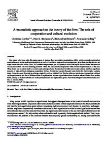
Figure 1. The average productivity of labor function f(k) and the marginal productivity of labor function f(k)kf’(k) with respect to the capital-labor ratio k

JSSM

The Theory of the Revenue Maximizing Firm it can be indicated with kw, so that we have: f (k w ) = w

175

maximization program: (14)

Maximize Q(K0, L)

Both these conditions are shown in figure 1, where the functions f(k) and QL = f (k ) − kf ' (k ) are depicted. Since

subject to Q(K0,L) − wL ≥ r0 K 0 .

f’(k)>0, we deduce that QL always stays below f(k). Once the real wage rate w and the level of capital K 0 are given, the profit maximizing firm is in equilibrium at the point B, ∧

∧

∧

'

where f (k ) − k f (k ) = w . In this point, the output per ∧

worker is f ( k ) , so the profit per worker is given by the difference:

(20)

The Lagrangian of this problem is: ℑ = Q ( K 0 , L) + λ [Q ( K 0 , L) − wL − r0 K 0 ]

(21)

from which we derive the following Kuhn-Tucker conditions: ∂ℑ = QL + λ (QL − w) = 0 ∂L

(22)

(15)

∂ℑ = (Q − wL − r0 K 0 ) ≥ 0, λ ≥ 0, λ (Q − wL − r0 K 0 ) = 0 (23) ∂λ

If we indicate with r the rate of profit or the rate of net return on capital, so that:

Q − wL − r0 K 0 >0, from (23) we have λ = 0 and from

∧

∧

'

∧

f (k ) − w = k f (k )

r=

Q − wL f (k ) − w = K k

(16)

then, from equation (15) we deduce that the maximum ∧

rate of profit r is given by: ∧

∧

r=

f (k ) − w ∧

∧

= f ' (k )

If

the

constraint

λ=

k

which says that r is equal to the marginal productivity of

rw =

f (kw ) − w =0 kw

∧

the profit maximizing one k . If w increases, both ratios ∧

k w and k increase, and their difference increases too.

2.2. The Equilibrium Conditions with a Minimum Acceptable Return on Capital Constraint If we introduce a minimum acceptable return on capital constraint of the form: Q − wL f (k ) − w = ≥ r0 K0 k

Copyright © 2008 SciRes

is

if

(24)

(25)

which says that the rate of return on capital must be equal to the minimum acceptable rate. This condition can be put in the form: f ( k ) − kr0 = w

(26)

If we consider that the range of r0 is: 0 ≤ r0 ≤ f ' ( k )

(27)

it follows that the curve f (k ) − kr0 has an intermediate mapping between f(k) and f (k ) − kf '(k ) , as it is depicted in figure 2(a). Given the level of capital K 0 , the real wage rate w and the minimum acceptable return on capital r0 , the equilibrium point of a revenue maximizing firm is no more A, but A’, where equation (26) is satisfied. Let k0 = K 0 /L0 be the capital-labor ratio which satisfies equation (26), in point A’ the output per worker of the firm is f (k0 ) . Clearly, at this point the rate of return on capital is: r0 =

(19)

then a revenue maximizing firm solves the following

that

QL w − QL

Q − wL = r0 K0

(18)

Each level of w corresponds to a minimum capitallabor ratio k w for which we have a null rate of profit. Given the amount of capital, the firm employs more labor if it maximizes revenue than if it maximizes profits; and this explains why the equilibrium ratio k w is smaller than

binding,

while, from the condition Q − wL − r0 K 0 = 0 , we have:

∧

capital corresponding to the optimal capital-labor ratio k . A revenue maximizing firm is in equilibrium at point A, where the average productivity of labor equals the real wage rate, that is f ( k w ) = w . At this point the profit rate is zero, as we have:

not

equation (22) we deduce that QL = 0, hence the firm does not produce anything. If on the contrary the firm does produce something, the constraint is binding, so that Q − wL − r0 K 0 = 0 and λ >0. In this case, from equation (22) we have:

(17)

∧

is

f ( k0 ) − w k0

(28)

∧

where k w ≤ k0 ≤ k . When r0 varies between zero and

JSSM

Beniamino Moro

176

f ' (k ) , the equilibrium point A’ ranges between A and B,

while the equilibrium capital-labor ratio ranges between ∧

k w and k . In figure 2(b), both the revenue-capital ratio Q / K 0 (which is equal to the output-capital ratio, because

P=1) and the rate of profit r are depicted. The rate of profit varies with respect to k according to the rule:

f (k ) − w (29) k For each level of w and K 0 , the rate of profit varies as r (k ) =

follows. In the interval 0≤ k< k w , it is negative and increases with respect to k, ranging from −∞ to zero. In the ∧

interval k w ≤ k ≤ k , it is positive and increasing, and

f (k )

C

∧

f (k )

f (k )

C'

f ( k0 )

f (k w ) = w

f ( k ) − kr0

A

f ( k ) − kf '(k )

A'

B

(a)

0 Q , K0

k (b)

r

f (k w ) / k w f (k0 ) / k0 Q / K 0 = f (k ) / k

∧

r r0

r (k )

0 kw

k0

∧

k

k

Figure 2. The mapping of the revenue-capital ratio (output-capital ratio) Q/K0 and the rate of profit r(k) with respect to k

Copyright © 2008 SciRes

JSSM

The Theory of the Revenue Maximizing Firm ∧

varies between zero and its maximum value r given by: ∧

∧

r=

f (k ) − w

(30)

∧

k ∧

Finally, in the interval k < k< ∞ , it is positive and decreasing, and tends asymptotically to zero for k→ ∞ . From figure 2(b), we see that for k= k w the rate of pro∧

∧

fit r is zero, for k= k it takes the maximum value r , while for k= k0 it equals r0 . In figure 2(b), the revenue-capital ratio or output-capital ratio Q K 0 = f (k ) / k is also depicted. Given the level of capital K 0 , this increases with respect to L, so it decreases with respect to the capital-labor ratio k. Using de L’Hôpital’s rule we have: d f (k ) f (k ) dk lim = lim = lim f ' (k ) = ∞ d k →0 k k →0 k →0 k dk lim

k →∞

(31)

f (k ) = lim f ' (k ) = 0 k →∞ k

(32)

so the ratio f(k)/k ranges between infinity and zero for 0< k< ∞ . Furthermore, we can check if the sign of its derivative is negative: d f (k ) = − [ f (k ) − kf '(k )] k 2 < 0 dk k

(33)

But for k< k w the ratio Q K 0 = f (k ) / k does not make sense, because it does not respect the non bankruptcy constraint. On the contrary, for k≥ k w , this ratio is economically meaningful and decreases with k, tending asymptotically to zero as k → ∞ . Hence, its maximal economically meaningful value Qw / K 0 = f (k w ) / kw corresponds to a capital-labor ratio equal to k w .

mum acceptable return on capital constraint of the form r ≥ r0, then the equilibrium point is A’ in figure 2(a), where f (k ) − kr0 = w. Given the level of capital K 0 , the employ∧

ment in point A’ is equal to L0 for which L ≤ L0≤ Lw and k0= K0/L0. Therefore, in this point equation (28) is verified. ∧

Thus, if r0 increases from zero to r , the equilibrium point A’ moves along the segment AB, going away from point A to point B. Point A’ is as far from point A as higher the minimum acceptable return on capital r0 is. An optimal level of the capital-labor ratio k0 for which ∧

k w ≤ k0 ≤ k corresponds to each predetermined level of r0 . Given the level of capital K0, this also corresponds to ∧

an employment level L0 for which L ≤ L0≤ Lw, where Lw is the maximum level of employment compatible with the ∧

respect to the non bankruptcy constraint and L is the level of employment that maximizes the rate of profit. Introducing a minimum acceptable rate of return on capital amounts to introduce a limit to the expansion of the production and the employment of the firm.

2.3. A Generalization of the Static Theory of a Revenue Maximizing Firm Once we have proven that, given the absolute value of capital K 0 , the profit maximization of a firm amounts to the maximization of the rate of profit (or the rate of return on capital), while the maximization of the revenue amounts to the maximization of the revenue (or output) per unit of capital, these results can be generalized for each given level of capital K 0 . So, the equilibrium conditions, both for a profit or for a revenue maximizing firm, become independent from the absolute value of capital and labor employed in the production process. They only depend on the capital-labor ratio. Therefore, if we define:

Therefore, once the level of capital K0 is given, if the objective function of the firm is to maximize profits, this corresponds to maximize the rate of profit. In this case, ∧

the optimal quantity of labor to be employed is L for ∧

∧

which k = K 0 / L and the equilibrium point is B in figure 2(a). On the contrary, if the objective function of the firm is to maximize revenue, this corresponds to maximize the revenue or output per unit of capital. In this case, the op∧

timal quantity of labor to be employed is Lw > L for which ∧

k w = K 0 /Lw and k w < k . Then, the equilibrium point is A

in figure 2(a), which corresponds to the maximum level of employment compatible with the respect of the non bankruptcy constraint. If the revenue maximizing firm must respect a miniCopyright © 2008 SciRes

177

r=

Q − wL f (k ) − w = K k

(34)

as the rate of profit (or the rate of net return on capital), then the program of a profit maximizing firm becomes: Maximize subject to

Q − wL K

(35)

Q ≥0 K

The Lagrangian of this problem takes the form: ℑ=

Q − wL Q +λ K K

(36)

from which the following Khun-Tucker conditions can be derived:

JSSM

Beniamino Moro

178 ∂ ℑ KQK − (Q − wL) λKQK − λQ =0 = + ∂K K2 K2

(37)

∂ ℑ QL − w λQL = + =0 K K ∂L

(38)

∂ℑ Q Q = ≥ 0, λ ≥ 0, λ = 0 ∂λ K K

(39)

ing, that is if Q−wL>0, then from (48) we deduce λ =0. In this case, from equation (50) we have QL =0, which implies:

(40)

(1+ λ ) QL =w

(41)

If the firm produces, then Q/K>0 and from equation (39) we deduce that λ=0, thus equations (40) and (41) take the form: Q−K QK = wL → f (k ) − kf ' (k ) = w

(42)

QL = f ( k ) − kf ' (k ) = w

(43)

These two equations state the same maximization rule, corresponding to the equality of the marginal productivity of labor to the real wage rate. This again re-asserts that the equilibrium capital-labor ratio for a profit maximizing

(51)

f(k)= kf ' (k )

(52)

or:

Equations (37) and (38) can also be stated in the form: (1+ λ ) [Q − KQK ] = wL

QL = f ( k ) − kf '(k ) =0

This last equation is satisfied only for k=0, that is, when the firm does not produce anything. Analogously, for λ =0, also equation (49) leads to the same conclusion. In fact, if λ =0, then Q=K QK , and dividing by L we obtain (52). It follows that, if the firm produces, the non bankruptcy constraint must be binding, which implies: Q−wL=0 → f(k)=w

In this case, from (48) we deduce that λ >0 and the value of λ can be determined either from (49) or (50). Using the latter, we have: (1+ λ )[ f (k ) − kf ' (k ) ]= λ f(k)

∧

λ=

Maximize subject to

Q K

(44)

where the firm respects a non bankruptcy constraint. To solve this problem, let us form the Lagrangian function: ℑ=

Q λ (Q − wL ) + K K

(45)

from which the following Kuhn-Tucker conditions can be derived: ∂ ℑ KQK − Q λ [KQK − (Q − wL)] = + =0 ∂K K2 K2

(46)

∂ ℑ QL λ (QL − w) = + =0 ∂L K K

(47)

∂ ℑ Q − wL λ (Q − wL) = ≥ 0, λ ≥ 0, =0 K K ∂λ

(48)

Equations (46) and (47) can be put in the form:

'

kf (k )

(49)

(1+ λ ) QL = λ w

(50)

respectively. If the non bankruptcy constraint is not bind-

=

QL kQK

(55)

which defines the equilibrium value of λ . Equation (55) can also be put in the form: QL = λk QK

(56)

where MRS L / K stays for the marginal rate of substitution between labor and capital. If we interpret λ as the shadow price of capital, then (56) means that in equilibrium the marginal rate of substitution must equal the shadow value of per capita capital. As we shall see later, this rule also applies in a dynamic analysis. Because equations (53) and (56) are satisfied for k= k w , it is confirmed that the equilibrium capital-labor ratio for a revenue maximizing firm is k w , that is the value of k which guaranties the equality between the average productivity of labor and the real wage rate. Finally, if the firm must satisfy a minimum return on capital constraint, the maximization program is as follows: Maximize subject to

(1+ λ ) (Q−K QK )= λwL

Copyright © 2008 SciRes

f ( k ) − kf ' ( k )

MRS L / K =

Q − wL ≥0 K

(54)

The same result is obtained from (49) dividing by L. From (54) we have:

firm is k . Likewise, the program of a revenue maximizing firm becomes:

(53)

Q K

(57)

Q − wL ≥ r0 K

where r0 is the minimum acceptable rate of return on capital. The Lagrangian of this problem is: ℑ=

Q ⎡ Q − wL ⎤ + λ⎢ − r0 ⎥ K K ⎣ ⎦

(58)

JSSM

The Theory of the Revenue Maximizing Firm from which we derive the following Kuhn-Tucker conditions:

179

∂ ℑ KQK − Q ⎡ KQK − (Q − wL) ⎤ = + λ⎢ ⎥=0 ∂K K2 K2 ⎣ ⎦

(59)

∂ ℑ QL λ (QL − w) = + =0 K ∂L K

(60)

capital-labor ratio for a revenue maximizing firm, when a minimum rate of return on capital constraint must be satisfied, is k= k0 . To this value of k we have the balance between the average productivity of labor, net of the minimum acceptable rate of return on capital, and the real wage rate. This condition is also obtained in the following dynamic analysis.

∂ ℑ Q − wL ⎡ Q − wL ⎤ = − r0 ≥ 0, λ ≥ 0, λ ⎢ − r0 ⎥ = 0 (61) K ∂λ K ⎣ ⎦

3. The Dynamic Analysis of the Revenue Maximizing Firm

Given that equations (59) and (60) are similar, respectively, to equations (46) and (47), they can again be put in the form of equations (49) and (50). From (61) we can conclude that, if the minimum rate of return on capital constraint is not binding, then λ =0. In this case, equations (51) and (52) follow, and k=0. On the contrary, if the firm does produce, the minimum rate of return on capital constraint must be binding. Therefore, it must be:

3.1. The Equilibrium Conditions without a Minimum Acceptable Return on Capital Constraint

r0 =

Q − wL f ( k ) − w = K k

(62)

or f (k ) − kr0 = w

(63)

and λ is positive. In this case, either from (49) or (50), we conclude that (1+ λ )[ f (k ) − kf ' (k ) ]= λ [ f (k)−kr0]

(64)

and λ=

which

is

'

f (k ) − kf (k ) '

k[ f (k ) − r0 ]

positive

=

QL k (QK − r0 )

∧

for k < k , as

the

(65) difference

Equation (65) can be put in the form: QL = λk QK − r0

(66)

which states the equilibrium condition for a revenue maximizing firm in the case that a minimum rate of return on capital constraint must be satisfied. In this case, the equilibrium rule becomes the equality of the net marginal rate of substitution between labor and capital ( NMRS L / K ), which is a function of r0 , to the shadow value of per capita capital λ k. Now, the NMRS L / K is defined as the ratio of the marginal productivity of labor over the marginal productivity of capital net of the minimum acceptable rate of return r0 . Since equations (63) and (66), as is shown in figure 2, are satisfied for k= k0 , it is confirmed that the equilibrium

Copyright © 2008 SciRes

⎡

⎤

⎣

⎦

Q = Q ⎢ K (t ), L(t )⎥

(67)

where Q has the same properties as in a)-c) of section 2.1. Let P be the price of the output, so the instant revenue is PQ. The objective function of a revenue maximizing firm then is the present value (PV) of all future revenues, that is PV =

∫

∞

0

⎡ ⎤ PQ ⎢ K (t ), L(t )⎥ e −ρt dt ⎣ ⎦

(68)

where ρ is the instantaneous discount rate. The dynamics of capital accumulation can be defined as follows:

f '(k ) − r0 = QK − r0 is also positive.

NMRS L / K (r0 ) =

In the dynamic analysis, K, L and Q are all functions of time t. Therefore, the instant dynamic production function is

K& = α {PQ[K (t ), L(t )] − WL}

(69)

where K& = dK/dt is the net instantaneous investment (there is no depreciation of capital), while W is the nominal wage rate. Finally, 0≤ α ≤1 is the share of instantaneous profits the firm decides to accumulate. Normalizing P=1 so as w=W/P=W indicates both the real and the nominal wage rate, equation (69) must satisfy the condition: K& = α (Q−wL) ≥0

(70)

which is both the law of motion of capital and the instantaneous non bankruptcy constraint. Starting from an initial level of capital K 0 , the program of the revenue maximizing firm is Maximize

∫

∞

0

Q ( K ,L)e − ρt dt

(71)

subject to K& = α (Q-wL) ≥0, 0≤ α ≤1, and K(0)= K 0 , K ∞ free, K 0 , w given.

JSSM

Beniamino Moro

180

In this problem, K is the state variable while L is a control variable. What about α , which is the share of instantaneous profits the firm decides to accumulate?4 In fact, we can suppose that the firm can decide in each instant of time to accelerate the speed of capital accumulation by increasing the value of α . We have the maximum speed if α =1, while there is no capital accumulation if α =0. In the latter case, all profits are distributed to the stockholders. Hence, it is obvious to consider α as a second control variable of the problem. To solve the program (71), let us indicate with H C the current value Hamiltonian: H C = Q ( K , L) + λα (Q − wL)

(72)

where λ is a dynamic Lagrangian multiplier. Furthermore, as the costate variable is strictly adherent to the state variable K, λ can also be interpreted as the shadow price of capital. Because the Hamiltonian is linear with respect to α , the maximization rule ∂ H C / ∂ α = 0 does not apply in this case. Instead, we have a maximum in one of the extreme values of the α interval [0, 1]. Moreover, since λ is positive, as we will see later, H C is maximized for α =1 if Q−wL>0, while, for Q−wL=0, α is indeterminate. Furthermore, since Q is a strictly quasi-concave function, the Hamiltonian H C is a concave function of K and L. So, the following conditions of the maximum principle are necessary and sufficient for the solution of the program (71): ∂ HC = QL + λα (QL − w) = 0 ∂L

(73)

∂ HC K& = = α (Q − wL )

(74)

∂λ

λ& = −

∂ HC + ρλ = −QK − λαQK + ρλ ∂K

lim H C e − ρt = 0, lim λe − ρt = 0

(75)

in the employment of the labor factor, which corresponds to condition (9) and conditions (22) or (24) from a static point of view. This rule requires that the firm must balance the ratio of the marginal productivity of labor over the wage rate, net of the same marginal productivity of labor, to the shadow price of capital along the entire time path of the costate variable λ . Condition (74) again represents the dynamics of capital, while condition (75) is the equation of motion of the costate variable λ . Equations (74) and (75) together form the Hamiltonian or canonical system. Finally, equations (76) are the transversality conditions. The first one requires the limit of the present-value Hamiltonian vanishes as t→ ∞ . The second one requires the shadow price of capital in discounted value vanishes as t→ ∞ . Since the term e − ρt →0 as t→ ∞ , both these transversality conditions are satisfied for finite values of HC ≠0, and λ ≠0. This will be demonstrated in section 3.4. Condition (74), dividing by L and remembering that α =1, can be put in the form: K& = f (k ) − w L

(78)

Since from the definition of k=K/L we have K=kL, and K& = k& L+k L& , dividing by L and substituting we obtain: K& & L& = k + k = f (k ) − w L L

(79)

L& k& = f (k ) − w − k L

(80)

and finally:

Given the real wage rate w, equation (80) describes the dynamics of the capital-labor ratio as a function of the & L . Analogously, from rate of growth of employment L/ condition (75), setting α =1, we obtain: λ& = λ [ ρ − f '(k )] − f '(k )

(81)

(76)

which describes the dynamics of λ , given ρ , as a function of the capital-labor ratio.

Condition (73) guarantees the employment of the labor factor is optimized along the time path L(t). If the firm does make profits, Q−wL>0 and α =1, and from condition (73) we obtain:

Conditions (77), (80) and (81), taken together, form a system of three equations, two of which are differential

t →∞

λ=

t →∞

QL f (k ) − kf ' (k ) = w − Q L w − [ f (k ) − kf ' (k )]

(77)

This is the dynamic optimization rule the firm follows 4

In Leland’s model [28], α is an exogenous parameter on which the firm exerts no influence. This assumption is not realistic and, at the same time, it contributes to limit Leland’s analysis.

Copyright © 2008 SciRes

equations, in three unknowns, given by k, λ and L&/ L . These equations fully describe the dynamics of a revenue maximizing firm. Given the real wage rate w and the discount rate ρ , we can find a steady state equilibrium for k& = λ& = 0 . This equilibrium is characterized by a time

constant value of the triple (k, λ , L&/ L ). Furthermore, our system can be decomposed into two sub-systems: the first one made up by equations (77) and (81), where the vari& L does not appear, and the second one correable L/

JSSM

The Theory of the Revenue Maximizing Firm sponding to equation (80) alone, which is the only equation where the employment rate of growth L&/ L is present. So, the first subsystem made up by equations (77) and (81) can be solved autonomously, and its solution gives, for λ& = 0, the steady state values of k and λ . Substituting the equilibrium value of k in equation (80) and setting k& = 0, the second subsystem yields the equilib& L. rium growth rate of employment L/ Now, let us concentrate, first of all, on the subsystem made up by equations (77) and (81), which can be depicted in a phase diagram on the plane k, λ . To construct this, we must pay attention to equation (77). Like in the ∧

static analysis, let us indicate with k the capital-labor ratio which satisfies the equality between the marginal productivity of labor and the real wage rate, that is ∧

∧

∧

QL = f ( k ) − k f ' ( k ) =w; and let us indicate with k w the

capital-labor ratio which satisfies the equality between the average productivity of labor and the real wage rate, that is f ( k w ) = w . From equation (77), since QL →0 as k→0,

181

However, equation (77) is not economically meaningful for 0≤ k< k w , because in this range the non bankruptcy constraint is not satisfied. Anyway, for k = k w , the firm does not make profits, so we have Q−wL=0 and α is indeterminate in the open range α ∈[0, 1) . In this case, from (73) we obtain: λ=

f (k w ) − k w f ' (k w ) QL = α [ w − Q L ] α [ w − f (k w ) + k w f ' (k w )]

(84)

where λ is defined with respect to α for k = k w . The mapping of the function Gw(k, λ) = 0 is depicted in figure 3. The part of this function that has an economic meaning ∧

belongs to the range [ k w , k ); for k = k w , the function Gw (k , λ ) = 0 becomes a truncated vertical line, where the truncation point A is given by: λ A = lim

k →k w

f (k ) − kf '(k )

(85)

w − [ f (k ) − kf ' ( k )]

whereas the ratio QL /(w− QL) → ∞ as (w− QL) →0 and

where the limit is calculated as k→ k w from the right. For

k→ k , we deduce that λ is an increasing function of k,

k w 0, and λ >0, so we have positive values of the shadow price of capital. Furthermore, always for values of k> k+, differentiating equation (86), we have: ∂ λ& /∂ k (1 + λ ) f " (k ) dλ 0, implying λ increases with respect to time, on the right of the λ& = 0 curve. Since the value of the capital-labor ratio at the point E is constant at the level k , from (80), which is the second subsystem that describes the dynamics of the revenue maximizing firm, we have: L& k& = f ( k ) − w − k = 0 L

(98)

from which we deduce: L& f (k ) − w = L k

(99)

Therefore, in the dynamic equilibrium of point E, the

JSSM

Beniamino Moro

184

growth rate of employment is given by the return on capital rate corresponding to the equilibrium capital-labor ratio k . As k is stationary, this implies that K grows at the same rate as L. Furthermore, the linear homogeneity of the production function implies that Q increases at the same rate, too. Thus, we have: L& K& Q& f (k ) − w = = = =r L K Q k

(100)

where r is the common growth rate of labor, capital and output. Therefore, in point E we have a balanced growth of the firm, where the rate of growth r is endogenously determined. Therefore, this is a neoclassical endogenous model of the revenue maximizing firm, which goes further beyond Leland’s analysis. There is no transitional dynamics in this model. In fact, if the firm begins its activity with the capital K(0)=K0, it must choose from the beginning the level L0 of the labor factor for which we have K0/L0= k and it must keep permanently fixed this capital-labor ratio. So, the equilibrium time path of k is constant. Analogously, the equilibrium time path of the shadow price of capital is also constant at the level indicated by (94), whereas the equilibrium time paths of labor, capital and output depend on the rate of endogenous growth r as defined by (100). They are defined respectively by the following exponential functions: L = L0 e r t

(101)

K = K 0 er t

(102)

Q = Q0 e r t

(103)

where, given K 0 , the value of L0 is defined by L0 = K 0 / k , whereas that of Q0 is given by Q0 =

Q( K 0 , L0 ). The k& = 0 curve given by (98) must plot as a vertical straight line in figure 5, with horizontal intercept k . In a neighborhood of point E along the Gw (k ,λ ) = 0 curve, the value of k, and not only that of λ , tends to depart from its equilibrium value. This can be demonstrated differentiating (80) with respect to k: .

∂ k& L = f ' (k ) − ∂k L

(104)

Substituting to L& /L its value given by (99), in a neighborhood of the point E we have: ∂ k& w − [ f (k ) − k f ' (k )] >0 = ∂k k

Copyright © 2008 SciRes

(105)

∧

which assumes a positive value because for k < k the real wage rate is greater than the marginal productivity of labor. This suggests that k& should follow the (−, 0, +) sign sequence as k increases. Hence the k-arrowheads should point leftwards to the left of the k& =0 curve, and rightwards to the right of it. This means that, for k< k , we have k& < 0, so k decreases with respect to time, while for k> k we have k& >0, so that k increases with respect to time. Therefore, along the Gw (k ,λ ) = 0 curve, the arrowheads point rightwards and upward to the right of the point E and they point leftwards and downward to the left of that point. So, both the capital-labor ratio k and the shadow price of capital λ , when moving along the Gw (k ,λ ) = 0 curve to optimize the use of labor, tend to increase to the right of point E and to decrease to the left. It follows that point E is dynamically unstable, and the firm can remain in equilibrium at that point only if it has chosen to stay there from the beginning. If, on the contrary, the firm begins its activity with a capital-labor ratio greater than k , the dynamics of the model suggests that the firm must choose a point on the right of point E along the Gw (k ,λ ) = 0 curve; so, it is induced to over-accumulate capital, approaching asymp∧

totically the capital-labor ratio k which maximizes the rate of profit. But, in this case, a dynamically efficient equilibrium point for a revenue maximizing firm does not ∧

exist, because when k tends to k the shadow price of capital tends to infinity, so it has not a stationary value. On the contrary, if the firm begins its activity with a capital-labor ratio smaller than k , the dynamics of the model suggests that the firm must choose a point on the left of the point E along the Gw (k ,λ ) = 0 curve. So, it is induced, following the arrowheads, to under-accumulate capital moving along this curve towards the point A. In the point A, the value of α becomes indeterminate in the open interval 0≤ α r must be satisfied, which implies that r < r . This ∧

which can also be put in the form: MRS L / K =

k w ρ Max

=

to the (17), we have r = f '(k ) , from the definition of k+

(107)

ρw

w

∧

while the value of λMax , remembering equation (91), is given by: λMax =

λ A = λMax =

185

also implies that the case k = k , when the equilibrium points of a revenue maximizing firm and of a profit maximizing firm should coincide, does not exist. In fact, ∧

we always have k < k . Referring once again to figure 5, we can summarize the following cases: ∧

- for ρ ≤ r , no equilibrium of the revenue maximizing firm exists; ∧

- for r < ρ ≤ ρ + , we have a unique equilibrium of endogenous growth corresponding to the stationary point E = (k , λ ) in figure 5; - for ρ + < ρ < ρ w , we have an endogenous growth equilibrium in point E of figure 5 and multiple stationary equilibria without growth corresponding to the interval BB’ in the same figure; - for ρw≤ ρ < ρ Max , we only have multiple stationary equilibria without growth in the interval AB’, being A, in this case, over B; - for ρ = ρ Max , we have a unique stationary equilibrium without growth corresponding to point A=B’; JSSM

Beniamino Moro

186

- for ρ > ρ Max , again no equilibrium of the revenue maximizing firm exists.

infinity, while the instantaneous rate of profit varies with respect to k from − ∞ to zero in the interval 0< k ≤ k w , it

3.4. The Present Value, the Net Present Value per Unit of Capital and the Transversality Conditions

becomes positive and increasing in the range k w < k < k ,

∧

∧

In general, for P=1 and r < ρ ≤ ρ Max , the present value (PV) of future revenues of the firm is: PV =

∫

∞

0

Lf ( k )e − ρt dt

(112)

∧

⎡

⎤

∧

further it assumes its maximum value r = ⎢ f (k ) − w⎥ ⎣

⎦

∧

k

∧

for k= k , and then it decreases towards zero as k→ ∞ . As a consequence, the ratio NPV/K0 also varies from − ∞ to zero in the interval 0< k ≤ k w , it becomes positive and ∧

where L=L0ert and L0=K0/k, while r is any endogenous

increasing in the range k w < k< k , further it assumes its

growth rate which must be smaller than r . Substituting we have:

maximum value for k = k , and then it decreases towards zero as k→ ∞ . The mapping of r with respect to k is also depicted in figure 7(c). This corresponds to the mapping of the rate of profit in the static analysis.

∧

PV =

∫

∞

0

L0 f (k )e − ( ρ − r )t dt

(113) ∧

It is clear that PV converges only if ρ >r. As ρ > r >r, this condition is satisfied. Dividing (113) by K0, we obtain the present value of future revenues per unit of initial capital: PV = K0

∫

∞ 0

f ( k ) − ( ρ − r )t e dt k

(114)

Given K 0 , when L0 varies between infinity and zero, the capital-labor ratio k varies between zero and infinity, while the instantaneous output per unit of capital f(k)/k, remembering (33), varies between infinity and zero, decreasing with respect to k. But, for k< k w , the ratio f(k)/k is not economically meaningful, because it does not respect the non bankruptcy constraint. Whereas for k≥ k w , as in the static analysis, the ratio f(k)/k is economically meaningful. It decreases with k and tends asymptotically to zero as k→ ∞ . So, its maximum value is given for k= k w , as we can see in figure 7(c). In the same way, we can define the net present value NPV as follows: NPV =

∫

∞

0

[Lf (k ) − wL] e

− ρt

where L=L0e and L0= K 0 /k. This equation can be put in the form:

∫

∞

0

L0 [ f (k ) − w] e − ( ρ − r )t dt

(116)

∧

which is convergent as ρ > r >r. Dividing (116) by K 0 , we obtain the net present value per unit of capital: NPV = K0

∫

∞

0

∞ f ( k ) − w − ( ρ − r )t e dt = re − ( ρ − r )t dt k 0

lim H c e − ρ t = 0

(118)

lim λe − ρ t = 0

(119)

t →∞ t →∞

which must be satisfied along the optimal paths of the involved variables. It is immediate to verify the (119), as in equilibrium we have λ = λ , where λ is constant if the firm has an endogenous growth equilibrium in point E of figure 5, whereas it takes a value which ranges between λ B and λ Max if the firm is in a stationary equilibrium corresponding to the capital-labor ratio k w . In both cases, as the term e− ρ t → 0 for t → ∞ , condition (119) is satisfied. To verify condition (118), we need to write it in the extended form: lim [ Q + λ α ( Q − wL )] e − ρ t = 0

t→∞

∫

(120)

If we have a stationary equilibrium, Q and L are constant, so equation (120) is satisfied. If, otherwise, we have an endogenous growth equilibrium, then Q = Q0 e

rt

and

L = L0 e rt , where r = [ f (k ) − w] / k is the endogenous growth

rate. Substituting these values, the condition (120) becomes: lim Q0 + λα (Q0 − wL0 ) e − ( ρ − r ) t = 0 (121) t →∞

[

]

∧

(117)

As said, given K 0 , when L0 varies between infinity and zero, the capital-labor ratio k varies between zero and

Copyright © 2008 SciRes

∧

The condition ρ > r , which is necessary for the convergence of the objective integral, is also necessary and sufficient to satisfy the transversality conditions of our optimal control problem. These conditions are:

(115)

dt

rt

NPV =

∧

which is satisfied because ρ > r > r .

3.5. The Equilibrium Conditions with a Minimum Acceptable Return on Capital Constraint

JSSM

The Theory of the Revenue Maximizing Firm

187

f(k) f(k)

f (k ) − k r E

A

f (k ) − kf ' (k )

w B

(a)

0 k

λ λMax

B'

λB

B

Gw = 0 k& = 0

(b)

E −

λ

λ& = 0

A 0

k+

k

f (k ) / k , r f (k w ) / k w −

(c)

−

f (k ) / k

f (k ) / k

∧

r

−

r (k )

r 0 kw

−

k

∧

k

k

Figure 7. The endogenous growth dynamics of the revenue maximizing firm Copyright © 2008 SciRes

JSSM

Beniamino Moro

188

If the firm must respect a minimum acceptable return on capital constraint of the form: π

(122) ≥ r0 , for all t ∈ [0,∞ ] K where π = Q − wL is the instantaneous profit of the firm, then we must modify the optimal control problem to take account of this. As the constraint can also be expressed in the form: Q − wL − r0 K ≥ 0

(123)

the program of the revenue maximizing firm becomes: Maximize

∫

subject to

∞ 0

Q ( K , L)e − ρt dt

]

L& k& + k = f (k ) − w − r0 k >0 L

[

(134) (135)

]

λ& = − f '( k ) − λ f ' (k ) − r0 + ρλ

λ=

(124)

0≤ α ≤1

(136)

f (k ) − kf ' (k )

(137)

w − [ f ( k ) − kf ' (k )]

which is the same as (77). So, all observations just referred to the Gw ( k , λ ) = 0 curve also apply to (134).

Q − wL − r0 K ≥ 0

and K(0)=K0, K ∞ free, K0, w, r0 given. The current value Hamiltonian must, in this case, be extended to form a Lagrangian function in current value, which takes account of the new constraint (123). This Lagrangian is: ℑc = Q + λα (Q − wL − r0 K ) + γ (Q − wL − r0 K )

(125)

where λ and γ are two dynamic Lagrangian multipliers expressed in current values. As ℑc is concave in K and L, and it is linear with respect to α , the following conditions of the maximum principle are necessary and sufficient for the solution of the program (124): ∂ ℑc = QL + λα (QL − w) + γ (QL − w) = 0 ∂L

(126)

∂ ℑc = Q − wL − r0 K ≥ 0, γ ≥ 0, γ (Q − wL − r0 K ) = 0 (127) ∂γ ∂ ℑc K& = = α (Q − wL − r0 K )

(128)

∂ ℑc λ& = − + ρλ = −QK − λα (QK − r0 ) − γ (QK − r0 ) + ρλ ∂K

(129)

∂λ

Gw (k ,λ ) = f ( k ) − kf ' ( k ) + (λα + γ ) [ f (k ) − kf ' (k ) − w] = 0 (130) f ( k ) − w − r0 K ≥ 0, γ ≥ 0, γ [ f (k ) − w − r0 k ] = 0

(131)

L& k& + k = α [ f (k ) − w − r0 k ] L

(132)

]

λ& = − f ' (k ) − (λα + γ ) f ' (k ) − r0 + ρλ

As to λ& = 0 curve, it now depends not only on the discount rate ρ , but also on the minimum return on capital constraint rate r0 . In order to stress this dependence, from now on this curve will be indicated by the symbol λ&r = 0 . From (136), setting the stationarity condition, we obtain:

[

.

]

λ&r = − f ' (k ) + λ ( ρ + r0 ) − f ' (k ) = 0

(138)

from which we derive: λ ( λ&r =0) =

f '( k ) ( ρ + r0 ) − f '(k )

(139)

The only difference between this expression and (88) is that here we have ρ + r0 in the denominator instead of only ρ . Hence, introducing a minimum acceptable return on capital rate r0 is analogous to increasing the discount rate for the same amount. Therefore, let k++ be the level of k which satisfies the equation ( ρ + r0 ) − f ' (k ) = 0 , so that as k→k++ from the right we have λ → ∞ . Since f '(k ) decreases with k, for

and in addition we must maximize ℑc with respect to α . These conditions can be expressed in the following per capita form:

Copyright © 2008 SciRes

[

Gw (k ,λ ) = f (k ) − kf ' (k ) + λ f (k ) − kf '(k ) − w = 0

From (134) we obtain:

K& = α [Q − wL − r0 K ]

[

If the minimum acceptable return on capital constraint is not binding, from (131) we have γ =0. Furthermore, since ℑc is linear with respect to α , its value is maximized for α =1. In this case, the equations (130), (132) and (133) respectively reduce to:

(133)

k>k++ we have ( ρ + r0 ) − f ' (k ) >0, which implies λ >0. Furthermore, if we differentiate equation (138), we obtain: ∂λ& / ∂ k dλ − f " (k ) − λf " (k ) (1 + λ ) f " (k ) =− r =− =