Retrospective Theses and Dissertations
1988
The role of interest rate swaps in financial institutions David Olaf Vang Iowa State University
Follow this and additional works at: http://lib.dr.iastate.edu/rtd Part of the Finance Commons, and the Finance and Financial Management Commons Recommended Citation Vang, David Olaf, "The role of interest rate swaps in financial institutions " (1988). Retrospective Theses and Dissertations. Paper 8898.
This Dissertation is brought to you for free and open access by Digital Repository @ Iowa State University. It has been accepted for inclusion in Retrospective Theses and Dissertations by an authorized administrator of Digital Repository @ Iowa State University. For more information, please contact
[email protected].
INFORMATION TO USERS The most advanced technology has been used to photo graph and reproduce this manuscript from the microfilm master. UMI films the text directly from the original or copy submitted. Thus, some thesis and dissertation copies are in typewriter face, while others may be from any type of computer printer. The quality of this reproduction is dependent upon the quality of the copy submitted. Broken or indistinct print, colored or poor quality illustrations and photographs, print bleedthrough, substandard margins, and improper alignment can adversely affect reproduction. In the unlikely event that the author did not send UMI a complete manuscript and there are missing pages, these will be noted. Also, if unauthorized copyright material had to be removed, a note will indicate the deletion. Oversize materials (e.g., maps, drawings, charts) are re produced by sectioning the original, beginning at the upper left-hand corner and continuing from left to right in equal sections with small overlaps. Each original is also photographed in one exposure and is included in reduced form at the back of the book. These are also available as one exposure on a standard 35mm slide or as a 17" x 23" black and white photographic print for an additional charge. Photographs included in the original manuscript have been reproduced xerographically in this copy. Higher quality 6" x 9" black and white photographic prints are available for any photographs or illustrations appearing in this copy for an additional charge. Contact UMI directly to order.
University Microfilms International A Bell & Howell Information Company 300 North Zeeb Road, Ann Arbor, Ml 48106-1346 USA 313/761-4700 800/521-0600
Order Number 8909200
The role of interest rate swaps in financial institutions Vang, David Olaf, Ph.D. Iowa State University, 1988
UMI
300N.ZeebRd. Ann Arbor, MI 48106
The role of interest rate swaps in financial institutions
by
David Olaf Vang
A Dissertation Submitted to the Graduate Faculty in Partial Fulfillment of the Requirements for the Degree of DOCTOR OF PHILOSOPHY Major:
Economics
Approved
Signature was redacted for privacy.
In Charge of^Major Wo: Signature was redacted for privacy.
For the Signature was redacted for privacy.
For the Graduate College Iowa State University Ames, Iowa 1988
ii
TABLE OF CONTENTS Page GENERAL INTRODUCTION
1
Explanation of dissertation format SECTION I.
PLAIN VANILLA INTEREST RATE SWAPS: DESCRIPTION, REASONS, AND HISTORY
1 4
INTRODUCTION
5
DESCRIPTION OF INTEREST RATE SWAPS
6
REASONS FOR INTEREST RATE SWAP ACTIVITY
12
EVOLUTION OF THE INTEREST RATE SWAP
27
CONCLUSIONS
34
BIBLIOGRAPHY
35
SECTION II.
ON THE RELATIONSHIP BETWEEN INTEREST 38 RATE SWAPS AND CAPITAL IN SAVINGS AND LOAN INSTITUTIONS
ABSTRACT
39
INTRODUCTION
40
THEORETICAL MODEL
44
Predictions and results of the theoretical model
54
DESCRIPTION OF THE DATA SET
59
EMPIRICAL MODEL
66
EMPIRICAL RESULTS
70
BIBLIOGRAPHY
82
SECTION III.
DO INTEREST RATE SWAPS REDUCE THE EFFECT OF INTEREST RATE CHANGES ON COMMON STOCK RETURNS OF SAVINGS AND LOAN INSTITUTIONS?
83
iii
ABSTRACT
84
INTRODUCTION
85
MEASURING INTEREST RATE SENSITIVITY OF COMMON STOCK RETURNS FOR SAVINGS AND LOANS
88
MODELLING THE EFFECT OF INTEREST RATE SWAPS ON SENSITIVITY
91
Model building with path analysis
93
Path model
97
DESCRIPTION OF THE DATA SET
100
EMPIRICAL RESULTS
103
BIBLIOGRAPHY
116
SUMMARY CONCLUSION
117
ACKNOWLEDGMENTS
118
1
GENERAL INTRODUCTION This dissertation is on the role of interest rate swaps in the management of financial institutions.
More
specifically it concentrates on the use of swaps by savings and loan associations.
Since the stated purpose of interest
rate swaps is to hedge interest rate risk, the typical savings and loan association which holds a large proportion of its assets as long-term fixed-rate mortgages while using deposits to finance these assets may find the use of interest rate swaps to be valuable. Explanation of dissertation format This dissertation is divided into three main sections. Section I is essentially an introduction to the subject of interest rate swaps where the following topics are developed:
the mechanics of an interest rate swap, the
reasons for usage of swaps, and the history of how the instrument evolved.
An interest rate swap is an agreement
between two agents to trade interest payment obligations. The most powerful reason for the existence of interest rate swaps is the ability to hedge interest rate risk.
Interest
rate swaps evolved from the use of other instruments which were originally used to achieve this same goal. Section II provides a theoretical model relating the use of interest rate swaps and the level of capital in savings and loan associations.
This relationship between
2
swap usage and capital is then empirically estimated.
The
methodology involves the use of a two-equation, simultaneous, three stage least squares model.
The results
suggest that savings and loan associations tend to allocate more capital when they engage in swaps.
It is also
suggested that more capital leads to more swap market activity. The final section presents a test of whether interest rate swaps can reduce the fluctuation in stock prices of savings and loan associations caused by unanticipated interest rate changes.
The assets and the liabilities of a
savings and loan association are financial contracts which incur a change in value when the level of interest rates change, and as a result the stock price of the firm also changes.
If interest rate swaps are successful in reducing
the variability of the net interest income, then this effect should be reflected by less variability in the association's stock price.
The results of this section seem to suggest
that interest rate swaps have only an indirect effect in reducing stock price variability.
A possible explanation of
this limited success is the fact that swap usage is not public information and therefore market participants cannot directly distinguish between those savings and loan associations which are hedging themselves with swaps from those that do not. The general conclusions of this dissertation suggest
3
that interest rate swaps tend to be used more often by savings and loans which have higher capital levels and that interest rate swaps only have limited success in reducing stock price variability caused by unexpected interest rate changes.
4
SECTION I.
PLAIN VANILLA INTEREST RATE SWAPS: REASONS AND HISTORY
DESCRIPTION,
5
INTRODUCTION The first part of this section describes the simplest form of interest rate swap called the plain vanilla swap. The second part lists the reasons found in the literature for the existence of these instruments, and the third part reviews the history of how previous financial instruments evolved into interest rate swaps.
6
DESCRIPTION OF INTEREST RATE SWAPS An interest rate swap is an agreement between two parties to exchange interest payment obligations without exchanging the debt itself.1
Each firm is still responsible
for repaying its own debt because the swap contract is just a bilateral exchange of payments.
If one firm defaults on
its debt the other firm is not liable and merely returns to paying its original interest rate on its own debt.
The
amount of debt which they do not exchange but agree to switch interest payments on is called the notional principal. There are a number of different types of swaps, but the most typical is the fixed/floating rate swap sometimes known as the plain vanilla, coupon, or classic swap.2
in
this type of swap the first party promises to pay to the second at designated intervals a stipulated amount of interest calculated at a fixed rate on the notional principal; the second party promises to pay to the first at the same intervals a floating amount of interest calculated according to some floating-rate index on the same amount of notional principal.
The first party is called the fixed-
^Tanya S. Arnold, "How to Do Interest Rate Swaps," Harvard Business Review 62, No. 5 (September/October 1984): 96-101. ^Bank for International Settlements, Recent Innovations in International Banking (New York; Bank for International Settlements, April 1986), 37-60.
7
rate payer, and the second party is the floating-rate payer.3
Usually, a bank acts as an intermediary and
arranges the swap for the end-users.
Many times the end-
users are of different credit worthiness; therefore, one party may not agree to the swap unless the cash flows are guaranteed by the intermediary.
Under some cases, the
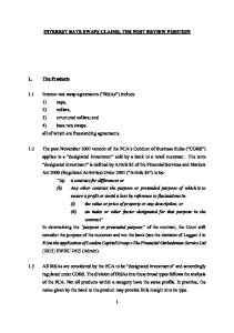
intermediary may become an end-user to both payers by making direct swaps to each party and in effect guarantee the cash flows in this way.^ To demonstrate how a plain vanilla interest rate swap works an example used by James Bicksler and Andrew H. Chen in their July 1986 article in the Journal of Finance will be repeated here. To illustrate, assume that a Baa corporation can borrow from banks at a floating rate equal to the T-Bill rate plus one-half percent and that an Aaa corporate borrower can borrow at a floating rate equal to the T-bill plus one-fourth percent. Also assume that in the bond market the quality spread between the two firms is 1.5% for a fiveyear bond. The Aaa firm would pay a fixed rate of 11.5% while the Baa firm would pay a fixed rate of 13%. That is, the corporate bond market requires a quality spread 1.25% larger than the short-term credit market. Thus, the two corporate borrowers can enter into an interest rate swap agreement and capture the economic benefits that result from savings in their costs of borrowing. The illustrative swap is detailed in Figure 2. 3James Bicksler and Andrew H. Chen, "An Economic Analysis of Interest Rate Swaps," Journal of Finance 41, No 3 (July 1986): 646-55. ^Recent Innovations in International Banking. 37-60.
8
Interest Rate 13%
Baa
T+1/2% 11.5% Aaa T+1/4% Short-term Figure 1.
Long-term
Demonstration of Quality Spreads
12% Baa
Aaa T-bill
T+1/2% (floating-rate market) Figure 2.
11.5% (fixed-rate market)
Direction of Payments in a Plain Vanilla Swap
9
The Aaa corporation issues a bond of $100 million at 11.5% and enters into a rate swap under which it is paid 12% in exchange for paying a six-month T-Bill rate. The net cost to the Aaa firm is the six-month T-Bill rate minus one-half percent, representing a saving of threefourths percent in raising the required amount of money in the floating-rate market. The Baa company borrows floating rate funds at the sixmonth T-Bill plus one-half percent and enters into the rate swap under which it pays a fixed rate of 12% and receives the T-Bill rate. Thus, the net fixed rate cost to Baa is 12.5%. In other words, the Aaa firm is raising 5-year money at the T-Bill rate minus one-half percent instead of having to pay one-fourth over the T-Bill rate, a net savings of .75%. The Baa firm is effectively raising 5-year money at a fixed rate of 12.5% (12% paid to the Aaa firm plus the .5% arbitrage cost on the floating rate funds). The combined savings of 1.25% shared by the two firms represent the quality spread differential. That is, the arbitrage opportunity between the two markets. The above example demonstrates the direction of the cash flows in a plain vanilla interest rate swap.
However,
this example is somewhat simplified from how swaps are conducted in the real world.
In the first place it assumed
that the two parties found each other by themselves.
In the
real world they probably would have gone through an intermediary and thus have to pay some sort of fee that would reduce the combined savings to something less than 1.25%.5
More importantly it should be pointed out that the
^Typically, an intermediary does this by selling a swap to one party and then selling an opposite swap to a party that wants the opposite position. The intermediary then collects the net difference that results from the cash-flows of the two swaps. Under market convention, the intermediary has an offer price and a bid price the difference of which is
10
combined reduction in borrowing costs of 1.25% is not necessarily all true savings. In the Bicksler and Chen exemple a Baa rated firm seems to have a net cost of 12.5% after the swap rather than the 13% it could get directly from the fixed-rate market. The Aaa rated firm nets a varieible rate of T-Bill minus onehalf percent, which is three-fourths percent below its direct borrowing cost from the variable-rate market.
These
reductions in borrowing costs are partially illusionary. For example, the Baa rated firm wanted long-term, fixed-rate debt.
Instead, it now has an obligation to pay a fixed
rate, but it still has short-term debt which has to be renewed.
Therefore, at least part of the .5% reduction in
borrowing is compensation for the Baa firm for not having a long-term commitment from its creditor. The Aaa firm supposedly ends up with floating-rate debt that is three-fourth percent cheaper than if it accessed the short-term market directly.
Again, the
question must be asked, does this firm really want long-term debt or was the reduction in the floating rate that it now pays a bribe to make the firm accept a long-term debt obligation over a short-term one?
Another reason why these
the spread that the intermediary collects. The offer price could be the rates at which the intermediary is willing to sell fixed-rate exposure, and the bid price could be the rates at which it sells variable-rate exposure. Recent Innovations in International Banking. 48.
11
cost reductions may be llluslonary stem from Bicksler and Chen's assumption that the long-term bond was not callable. In the real world many bonds are callcible while most swap contracts are not.
Therefore, in real world situations part
of the reduction in the effective interest rate could reflect the opportunity cost of the Aaa firm giving up its ability to call. Thus, the mere difference in quality spreads across maturities is not sufficient for a swap to be profitable. Instead* the difference in spreads must actually be quite large for such a swap to be beneficial to both parties ignoring any other reasons why the firms may want the swap. Suppose that in the above example the Baa firm was willing to engage in the swap and settle for short-term financing if its interest cost were one-half percent below its regular bond financing, suppose further that the Aaa firm may feel that a three-fourths percent reduction in its floating-rate interest cost is not adequate compensation for giving up its right to call its 11.5% fixed-rate debt and to replace it with cheaper fixed-rate debt should interest rates go down in the future.
If this were the case the combined 1.25%
difference in quality spread would not be a sufficient amount to allow both parties to benefit from such a swap.
12
REASONS FOR INTEREST RATE SWAP ACTIMTY Smith et al. listed four basic reasons why the interest rate swap market evolved.6
A possible fifth reason was
discovered later by Larry Wall.' (1) Profit opportunities from regulatory and tax arbitrage. (2) Lower transaction costs in managing exposure. (3) Financial market integration or completion. (4) What the literature calls classic financial arbitrage. (5) Reduction in agency costs.8 Examples of the first reason include: differing underwriting costs and policies toward bond registration, differing disclosure requirements in different markets, and different tax laws in different countries.
For example, in
the absence of a swap market a firm wishing to issue a bond of a particular currency denomination would have do so in the capital markets of that country and thus be sub]ect to its securities regulations and tax code.
The introduction
of the swap market allows for the separation of these effects, so that the firm could almost pick and choose which ^Clifford W. Smith, Jr., Charles W. Smithson, and Lee Macdonald Wakeman, "The Evolving Market for Swaps," Midland Corporate Finance Journal 3, No. 4 (Winter 1986): 20-32. 'Larry D. Wall, "Interest Rate Swaps in an Agency Theoretic Model With Uncertain Interest Rates," Working Paper. Federal Reserve Bank of Atlanta, July 1986. ®The first four reasons came from Clifford W. Smith et al., "The Evolving Market for Swaps," while the fifth reason came from Larry Wall's working paper.
13
regulation and tax code that it wished to be under.9 A specific example of the eUaove situation would be a previous Japanese policy to tax zero coupon bonds at the capital gains rate while having the tax payment delayed until maturity.
At that seune time the Japanese Ministry of
Finance was limiting the amount that pension funds could invest in non-yen-denominated bonds issued by foreigners.
A
U.S. firm could still borrow from the Japanese pension fund even with that limit and the pension fund could still get the tax benefit if the fund issued a zero coupon bond while making the appropriate swap such that the interest payment could be in yen and principal repayment in dollars.10 In general it is usually the case that if there are high fixed costs associated with using a particular market, then a larger or higher rated company will have the comparative advantage in borrowing from that market over a smaller or lower rated company.^
It should also be pointed
out that opportunities such as the Japanese pension fund example could theoretically continue to stimulate the swap market as long as differences in laws and tax codes continued to exist. The second reason, managing exposure, is probably the ^Smith et al., "The Evolving Market for Swaps," 24-6. lOlbid.. p. 25. llsicksler and Chen.
14
most important of the five.
Basically, when a firm has
assets and liabilities that are not of matched maturities it is exposed to interest rate risk.
For example, savings and
loan associations generally have long-term, fixed-rate mortgages as assets but fund these assets with short-term deposits.12
By entering into a swap as a fixed-rate payer
the savings and loan is essentially turning its variablerate deposits into fixed-rate financing.13
Such a use of
swaps could explain why the International Swap Dealers Association recently found that financial institutions accounted for 64.5% of its swap volume. In some cases it may be cheaper for a firm to hedge its interest rate exposure with a swap rather than use series of futures contracts.15 reasons for this.
There are two possible
First, each time one enters the futures
market there could be a transaction cost, and this cost could accumulate into a large amount especially if one needed a futures contract for each interest payment period 12J. Gregg Whitaker, "Interest Rate Swaps; Risk and Regulation," Economic Review; Federal Reserve Bank of Kansas City 72, No. 3 (March 1987); 3-13. 13lbid. l^International Swap Dealers Association, Quarterly ISDA Survey (International Swap Dealers Assoc., Inc., New York, Aug. 17, 1987). ISciifford W. Smith et al., "The Evolving Market for Swaps."
15
over the next several years.
Second, an interest rate swap
could be constructed to last for several years while futures contracts that extend that far into the future generally are not traded in the financial markets.
There therefore could
be high search costs in finding parties to hold the opposing position to such rare futures contracts.
Another possible
advantage of the swap over the futures contract is that if the correct swap partner is found, then the swap could be fashioned to fit the needs of the firm.
For example, the
floating-rate payments on the swap could be calculated according to any number of interest indexes.
A disadvantage
of swaps relative to futures contracts is that if one decides that hedging is unnecessary, one can merely stop buying or selling futures contracts, but to terminate a swap contract is much more expensive.
Therefore, the level of
swap market activity is limited to some extent by the relative cost of other such hedging vehicles and the prospect of future interest rate levels and stability. The third reason, financial integration, refers to the fact that interest rate swaps can allow participants to fill gaps left by missing markets.
For example, interest rate
swaps behave like a series of forward contracts—one forward interest rate contract made for each payment on one's notional principal for the desired length of time would give one the same result as a single interest rate swap contract
16
for that same length of time.
Therefore, a swap could be
used in place of a missing forward interest rate contract.16 The interest rate swap market also acts as a link between the capital and money markets because one swap participant may be borrowing from the money market and swapping interest payments with an agent who is borrowing from the capital market and vice versa.1?
The use of swaps could therefore
be used to artificially create a new instrument out of an old one that normally has a fixed rate by giving it a variable rate or vice versa.
Thus the swap market
synthetically completes or integrates the financial markets. The limit of this reason for swap activity could be almost unlimited so long as the need for new instruments increases. The fourth reason for the existence of swaps is that cost savings may be realized by financially arbitraging across different capital markets.IB
In the Bicksler and
Chen article the notion was advanced that the economic benefits in an interest rate swap result from the principle of comparative advantage.
The comparative advantage arises
from the possibility that there are some market IGibid. Julian Walmsley, "Interest Rate Swaps: The Hinge Between Money and Capital Markets," The Banker 135, No. 710 (April 1985): 37-40. IBciifford W. Smith, Jr. et al., "The Evolving Market for Swaps," p. 24.
17
imperfections that allow some borrowers to use some credit markets at a relatively cheaper cost than other borrowers.19 In other words, if prices in various financial markets are not mutually consistent, implying financial market inefficiency, then firms can reduce their cost of debt by borrowing in one place and swapping back.
These differences
in prices would have to come about from some sort of barrier that limits access to the cheaper markets. Arbitrage, in the classic sense, is the situation of taking advantage of different prices for the same product in different markets.
For example, the trading of currencies
to take advantage of a difference in exchange rates between three currencies is a case of arbitrage.
This could be done
without risk to the trader because she is just taking advantage of two different prices for the same product, currency in this case, by buying low in one market and selling high in another.^0
The financial arbitrage as
described in the literature with respect to interest rate swaps, however, is not necessarily risk free.
For example,
one firm may enter a swap for the purpose of hedging against interest rate risk for a certain number of years and if the swap partner defaults, the firm may have the cost of trying l^Bicksler and Chen. Z^Mordechai E. Krenin, International Economics. Third Edition (New York: Harcourt Brace Jovanovich, Inc., 1979), 37.
18
to replace that hedge under a different set of market conditions that may make a replacement swap more expensive than the original swap.
This could be an especially
expensive situation if the firm is pursuing a set of investment and financing plans that depend upon the swap for exposure management.
To avoid this problem an intermediary,
if there is one, could guarantee the cash-flows for a fee or by directly being an end-party to both firms.
In such a
case the end-users would not have to worry about assuming risk of the other party defaulting on the swap. One notion of financial arbitrage which was alluded to in the previous numerical example is that the smaller difference between higher and lower rated debt rates in floating-rate markets versus the difference in rates in the long-term markets represents an arbitrage opportunity to be exploited.21
This notion and the financial arbitrage
Z^The following citations explain or at least mention financial arbitrage of quality spreads across maturities. However, not all of these citations support this belief. Bicksler and Chen; Clifford W. Smith, Jr. et al., "The Evolving Market for Swaps," Midland Corporate Finance Journal 3, No. 4 (Winter 1986): 20-32; Jan G. Loeys, "Interest Rate Swaps: A New Tool for Managing Risk," Business Review; Federal Reserve Bank of Philadelphia (May/June 1985): 17-25; Trevor S. Ricards, "Interest Rate Swaps Offer Flexible Financing, Lower Interest Costs," Cash Flow 5, No. 10 (Dec. 1984): 37-39; Beth McGoldrick, "The Interest Rate Swap Comes of Age," Institutional Investor 17, No. 8 (Aug. 1983): 83-90; "Variations on a Theme of Swaps," The Global Swap Market: Euromonev (June 1986): 2-6; Gilbert M. Flick and Grant E. Sardachuk, "Interest Rate Swaps: Matches Arranged for Mutual Gain," CA Magazine 3, No. 3 (July 1985): 36-41; and Stuart M. Turnbull, "Swaps: A Zero
19
argument in general has since been criticized by Smith et al.,22 by Stuart
,23 and by
Turnbull
.24
Loeys
The numerical
example used previously in this paper called the difference in quality spreads an arbitrage opportunity to be exploited without considering that these differences may be a desired condition in the financial markets.25
The cost reductions
associated with interest rate swaps may then be more apparent than real. One of the first to make this observation was Jan Loeys.
Loeys mentioned in the Business Review that there is
a tremendous amount of evidence that suggests that financial markets are
26
efficient.
Therefore, the difference in
quality spreads for different maturities may exist for a Sum Game?" Financial Management 16, No. 1 (Spring 1987): 1521. 22ciifford W. Smith, Jr. et al., "The Evolving Market for Swaps." 23stuart M. Turnbull, "Swaps: A Zero Sum Game?" Financial Management 16, No. 1 (Spring 1987): 15-21. 24Jan G. Loeys, "Interest Rate Swaps: A New Tool for Managing Risk," Business Review; Federal Reserve Bank of Philadelphia (May/June 1985): 17-25. 25Bicksler and Chen; Trevor S. Ricards; Beth McGoldrick; Gilbert M. Flick and Grant E. Saradochuk; and Euromoney, "Variations on a theme of Swaps," The Global Swap Market; Euromonev (June 1986): 2-6. 2®a discussion of the evidence of market efficiency can be found in Thomas E. Copeland and J. Fred Weston, Financial Theory and Corporate Policy. Second Edition (Reading, Massachusetts: Addison-Wesley Publishing Company, 1983), 317-53.
20
valid reason.
For example, an investor would probably be
willing to lend money to a Baa rated company for a very short period of time, say three months, at a small interest premium over the rate for an Aaa rated company for the same period of time because should the company"s perceived position deteriorate the investor could simply refuse to renew the loan when the three months are up.
On the other
hand, in order to make a risk averse investor lend money on a long-term basis to a Baa rated company he must have a relatively large premium over that of an Aaa rated company for the same term;27 therefore, from the investors point of view the difference in quality spreads exists for a reason. In a similiar approach Clifford W. Smith et al. made the statement that the very process of exploiting any arbitrage opportunity should soon eliminate it.28
while
this is a more general criticism of the financial arbitrage argument and does not specifically address the quality spread difference idea that was presented by the Bicksler and Chen example, it does make the point that one would expect that firms try to go to the cheapest financing sources first.
If this were true, arbitrage opportunities
such as extremely large quality spread differentials would 27jan G. Loeys. 2®Clifford W. Smith, Jr. et al., "The Evolving Market for Swaps," p. 24.
21
not likely be left unexploited.
While there does appear to
be some evidence that quality spreads have become more equal in the early 1980s and that the profitability of plain vanilla swaps fell during that same time,29 quality spreads still do not equal each other.30 Stuart Tumbull made a similar observation in a recent Financial Management article that more closely addressed the Bicksler and Chen article.
His conclusion was that if
financial markets are competitive, not all parties to a swap can benefit.
If parties do benefit, then the growth in
swaps must be the result of externalities, possibly the incomplete markets externality as mentioned earlier.31 Tumbull's reasoning is as follows.
Suppose there are
two firms A and B where A wants to be the floating-rate payer and B, the fixed-rate payer. financial intermediary. (1)
There is also a
If markets are competitive, then
PVa(variable) = PVa(fixed) and
(2)
PVb(variable) = PVb(fixed).
Verbally this says that the risk-adjusted, present Z^Business Week, "Scrambling to Find New Markets for Interest Rate Swaps, "Business Week. 9 May 1983, 118. SOpederal Reserve Board of Governors, Federal Reserve Bulletin 68-72, Federal Reserve Board of Governors, Washington, B.C., 1982-1987. Slstuart M. Turnbull.
22
value cost to each company of using variable-rate debt is the same as the risk-adjusted, present value cost of using fixed-rate debt.
If this were not true, then the firm would
go to the cheaper source of funding, but such a difference would violate the competitive markets assumption. The condition for a swap to be beneficial to all parties involved is (3)
[PVa(fixed) - PVa(variable)] + [PVb(fixed) PVb(variable)] > PV + TC^ + TCj,
where PV is the economic profit that accrues to the financial intermediary and TC represents any additional net transaction costs to the firms.
This equation is very
similar to the Bicksler and Chen presentation except that the costs of debt are presented in present value form.
The
difference in borrowing costs in different markets for each firm must exceed the net transaction costs and the positive economic profit that the intermediary collects in order for the swap to benefit all three parties.
However, from the
competitive market assumption which is the basis for equations 1 and 2 and the assumption that TC and PV are positive, equation 3 simply cannot hold.
In Turnbull's
words, interest rate swaps are a zero sum game because not all three parties can benefit.3% From the criticisms presented by Loeys, Smith et al., 32Ibid.
23
and Turnbull it becomes clear that if markets are competitive and reasonably efficient, the notion of financial arbitrage of quality spreads across maturities as justification for plain vanilla interest rate swaps comes into doubt.
Unless there are externalities such as
different tax and regulatory treatments, geographic limits, or possibly agency problems such as the one that will be discussed next, it is unlikely that classic financial arbitrage can continue indefinitely as a source of swap market growth. Larry Wall of the Atlanta Federal Reserve may have discovered a possible fifth reason for swaps.
According to
Wall, interest rate swaps could be used to solve the problem of interest rate risk as well as an agency problem that could occur between stockholders and creditors within lower rated firms.33
Wall concluded that financing with long-term
non-callable bonds limits the interest rate risk problem that a firm would normally have if it financed with shortterm debt.
However, he also concluded that long-term bond
financing created an incentive for the firm to invest in suboptimal projects because the creditors do not have the ability to raise the rate on their bonds should the firm start to invest in risky projects after the bonds have been sold.
Essentially, the managers would be transferring 33Larry Wall.
24
wealth from the creditors to the shareholders by investing in risky projects.
Financing with short-term notes, on the
other hand, gives the firm the correct investment incentive because the creditors can adjust the risk premium each time the debt is renewed, but short-term debt exposes the firm to interest rate risk.
It therefore appears that a combination
of notes and swaps would solve this problem because if the firm was financing with short-term notes the changing risk premium would quickly discourage investing in poor quality projects.
At the same time the swap would reduce interest
rate risk by allowing the firm to be a variable-rate receiver.34 This firm's agency problem is solved only if the swap pays a floating rate based on some risk free index such as the rate on T-bills.
If the swap paid the total interest
expense, then the firm would not have the risk premium incentive to pick lower risk projects under Larry Wall's framework.35
Swap financing would be less expensive than
straight note financing if the cost of the incentive premium to get the other party to do the swap is less than the benefits of reduced interest rate exposure.
The reduced
exposure would reduce the probability of bankruptcy while the premium to get the other firm to enter the swap would 34lbid. 35ibid.. p. 14.
25
increase this risk.36
It is my conclusion that this premium
incentive is where Wall's agency theoretic model may be somewhat limited in explaining the existence of swaps because the model only looks at the effect of a lower rated firm that is trying to reduce its agency problem.
The size
of the premium incentive is not modelled from the other fiirm's point of view.
Considering the needs of the higher
rated firm and the possibility that it could have a similar agency problem of its own, the premium incentive to do the swap could be prohibitive.
However, Wall's observations
about the agency costs of short-term versus long-term debt could still be a contributing factor when used in conjunction with the other reasons for the existence of swaps. This section has just described the most typical interest rate swap the fixed/floating or plain vanilla swap and has listed and discussed five possible reasons for the existence of these instruments.
One of these reasons, the
financial arbitrage argument, has been considered to not be extremely valid by some researchers especially when the assumptions of efficient, competitive financial markets are made.
The other reasons at this time have not yet been
criticized in the literature.
While I would agree that
financial arbitrage is not a likely reason for the existence 36ibid.. p. 13.
26
of interest rate swaps, I would further conclude that all of the other reasons except managing interest rate risk are too specialized to have a significant effect on the growth of the swap market, and therefore, the major role of the interest rate swap today and in the future will be that of a hedging instrument, not an arbitraging device.
27
EVOLUTION OF THE INTEREST RATE SWAP The interest rate swap is basically a succession to the currency swap, and the currency swap was a successor to the back-to-back loan.
In a back-to-back loan two parties
in different countries make loans to one another, of equal value based upon the existing exchange rate, each denominated in the currency of the lender, and each maturing on the same date.3?
The payment flows are identical to
those of spot and forward currency transactions.
Back-to-
back loans were developed when exchange, controls were in force in the United Kingdom in the 1970s which in effect limited the access of residents and non-residents to each others capital markets.
In a back-to-back loan a means was
provided for non-residents to indirectly borrow fixed-rate 38
sterling.
After the abolition of exchange controls in
1979, they continued to be used as a means of creating or hedging long-term foreign currency exposure at lower costs than in the foreign currency
markets.39
The back-to-back loan had some disadvantages.
For
3"^Recent Innovations in International Banking. 37-60. 3Qibid. The existence of the back-to-back loan is an example of regulatory arbitrage (reason number 1). Interest rate swaps can be used today to circumvent such regulations. 39ibid. The reason that the back-to-back loan continued to exist after the regulations were lifted is the same as reason number two for the use of swaps today. The instrument was found to be a cheaper method of managing exposure than the standard techniques of that day.
28
example, in most cases each loan is a new debt obligation on the balance sheet.
Also the two loans are usually covered
by separate agreements.
If one party fails to make a
payment, the other may still be obligated to continue payments.40 The currency swap was developed to avoid most of these problems.
A currency swap is a transaction in which two
counterparties exchange specific amounts of two different currencies at the outset and repay over time according to a predetermined rule which reflects both interest payments and amortisation of principal.41
First among its advantages, a
currency swap does not increase the assets or liabilities on the balance sheet.
Second, it limits credit risk, since a
performance failure by one party relieves the other party of its obligations.
Thus, risk is limited to the cost of
replacing the expected income streams which depend upon interest and exchange rate movements.
These rates, however,
could very well have moved in a direction that would make the surviving party better off by the default of the other party.42
just like the back-to-back loan, government
restrictions stimulated the use of currency swaps by offering a way to indirectly access European capital markets 40ibid. 41ibid.. 37. 42ibid.. 38.
29
such as Eurobonds.43 The next step was the extension of the swap concept from the currency market to credit market instruments denominated in the same currency.
The paternity of this
breakthrough is hotly contested, but most observers agree that by 1982 interest rate swaps had grown beyond isolated deals to the point where one could speak of a market.*4
The
most common interest rate swap was the plain vanilla swap. Floating-rate payers were usually highly rated European banks, and fixed-rate payers were typically Baa-rated U.S. companies.45
it is believed by some that interest rate
swaps first emerged in the Eurobond market in late 1981.46 Large international banks which do most of their lending on a floating-rate basis, were involved in the first swaps so that they could use their fixed-rate borrowing capacity to obtain lower-cost floating rate funds.4?
Initially, the
swapping partners consisted mainly of utilities and lower43ibid.. 39. 44ibid. 45ibid. 46Jan G. Loeys, "Interest Rate Swaps: A New Tool, for Managing Risk," Business Review: Federal Reserve Bank of Philadelphia 62, No. 5 (May/June 1985): 17-25. 47it thus appears that the final step towards the development of the interest rate swap was instigated by reason number two, the use of the instrument to limit the exposure of European financial institutions.
30
rate industrial corporations that preferred fixed-rate financing.
During 1982, the first domestic interest rate
swap occurred between the Student Loan Marketing Association (Sallie Mae) and the ITT Financial Corp., with Sallie Mae making the floating-rate payments to ITT.^®
Since then,
swap volume grew to about $100 million during 1982,49 then exploded to $80 billion in 1984,50 to $140 billion in 1985,51 and then to over $200 billion in 1986.52
it should
be noted, however, that any figures dealing with the volume of interest rate swaps should be viewed with suspicion.
One
must remember that there are at least two, and most times, three parties in a swap.
Therefore, when interest rate swap
volume is reported it could be the case that both endparties and the intermediary may have reported their swap separately, and as a result, the swap may have been double or even triple counted. Complete data are not available for all of 1987 and 48jan G. Loeys. ^^Tanya S. Arnold, "How to do Interest Rate Swaps," Harvard Business Review 62, No. 5 (Sept/Oct 1984): 96-101. 50as estimated by Salomon Brothers in Economist. March 16, 1985, 30. Slciifford W. Smith, Jr., Charles W. Smithson, and Lee Macdonald Wakeman, "The Market for Interest Rate Swaps," Working Paper Series No. MERC 87-02. Managerial Economics Research Center, University of Rochester, New York, 1987. SZibid.
31
1988 but there has been some indication that the growth of newly issued swaps has slowed substantially from its previous pace, especially among savings and loan associations.53
In the meantime, interest rate swap
activity has reached the point where swaps have became a high volume, lower margin business, rather than the personalized, corporate financial deal that it originally was.54 Both investment banks and commercial banks have been active in arranging interest rate swaps.
They earn fees by
bringing the different parties together and by acting as settlement agents.
Settlement agents collect and pay the
net difference in the interest payments and serve as guarantor of the agreement.
Most intermediaries have gone
beyond their initial role of merely bringing different parties together by actually functioning as
^5
dealers.
in
other words, each party has an agreement only with the intermediary and is totally unaware of who might be on the other side of the swap.
The intermediary actually sells one
S^Office of Research and Statistics, Federal Home Loan Bank Board, Quarterly Financial Reports of Condition: Aaareaate Report of Each of the 12 Districts. Office of Research and Statistics, Federal Home Loan Bank Board, Washington, D.C., 1987-1988. 54k. Henerson Schuyler, "The Constraints on Trading Swaps," Euromonev (May 1985): 63-64. 55Jan Loeys.
32
party a swap without having the opposite swap with someone else at that particular time.
It holds the swap in
inventory in hope that another firm will later want a swap with the opposite position.
This arrangement has
facilitated the development of a secondary market in swaps, thereby increasing the liquidity of this instrument.
The
development of a secondary market, in turn, began to allow for the reversing, terminating, and general selling of existing swaps. In 1984 the typical swap involved a bond issue for $25 to $75 million with a 3 to 10 year maturity on one side, and a floating-rate loan on the other.5?
Since that time the
range of sizes and terms has widened.
Also, the floating
rate index typically used was the LIBOR (London Interbank Offered Rate); now different rates can be used such as the prime rate and the T-bill rate.®® Other variations on swaps began to develop at approximately the same time such as variable/variable rate swaps based on different indexes.
For example, a bank with
assets tied to the prime rate and liabilities based on LIBOR could use this tool to hedge itself.59
Another variation is
S^Recent Innovations in International Banking. 43. 57jan Loeys. 58ibid. 59lbid.
33
an interest rate swap across currencies which could be used by firms whose assets are denominated in a currency other than its liabilities.
It is also possible for firms to
exchange yields on their assets in much the same way they exchange interest payments on debt.^^ As a matter of speculation, there could have been some other contributing factors to the development of the interest rate swap market.
For example, the extremely high
level and volatility of interest rates that occurred during the period after 1979 when the Federal Reserve began targeting the money supply rather than interest rates®^ may have made interest rate swaps more attractive than ever before.
This would be especially true for financial
institutions such as banks and savings and loans which were undergoing a period of deregulation at approximately the same time.62
The higher rate volatility and the increased
freedom of action may have encouraged financial institutions to experiment with such instruments.
GOibid. ®^Dudley G. Luckett, Money and Banking. Third Edition (New York; McGraw-Hill Book Company, 1984). 62ibid.
34
CONCLUSIONS Interest rate swaps are a recent development in financial markets which allow firms to exchange interest rate payments on their debt.
There are known at the present
time five possible reasons why interest rate swaps exist. These reasons include tax and regulatory arbitrage, exposure management, classic financial arbitrage, and the reduction of agency costs within firms.
The development of the swap
market has its roots in the mid-1970s, and through constant modification and development the interest rate swap market exists as it is today.
The emphasis of the following two
essays will be on the exposure management aspect of swaps and its relationship to financial institutions, specifically savings and loan associations.
This is an important issue
that may play a role in the current debate of the regulation of interest rate swaps by financial institutions.63
63^o examples of regulation. Board of Governors Staff and the Federal Reserve Bank of New York, Treatment of Interest Rate and Exchange Rate Contracts in the Risk Asset Ratio. Board of Governors Staff and the Federal Reserve Bank of New York, March 3, 1987; Federal Home Loan Banks Interest Rate Swap. Cap. Collar and Floor Policy Guidelines. (Revision) Federal Home Loan Bank Board, Washington, D.C., March 10, 1987.
35
BIBLIOGRAPHY Arnold, Tanya S. "How to Do Interest Rate Swaps." Harvard Business Review 62, No. 5 (September/October 1984): 96-101. Bank for International Settlements. Recent Innovations in International Banking. New York: Bank for International Settlements, April 1986. Bicksler, James, and Andrew H. Chen. "An Economic Analysis of Interest Rate Swaps." Journal of Finance 41, No. 3 (July 1986): 646-55. Board of Governors Staff and the Federal Reserve Bank of New York. Treatment of Interest Rate and Exchange Rate Contracts in the Risk Asset Ratio. Board of Governors Staff and the Federal Reserve Bank of New York, March 3, 1987. Business Week. "Scrambling to Find New Markets for Interest Rate Swaps." Business Week. 9 May 1983, 118. Copeland, Thomas E., and J. Fred Weston. Financial Theory and Corporate Policy. Second Edition. Reading, Massachusetts: Addison-Wesley Publishing Company, 1983. Economist. 16 March 1985, 30. Euromoney. "Variations on a Theme of Swaps." Swap Market: Euromonev (June 1986): 2-6.
The Global
Federal Home Loan Banks Interest Rate Swap. Cap. Collar and Floor Policy Guidelines. (Revision) Federal Home Loan Bank Board, Washington, D.C., March 10, 1987. Federal Reserve Board of Governors. Federal Reserve Bulletin 68-72, Federal Reserve Board of Governors, Washington, D.C., 1982-1987. Flick, Gilbert M., and Grant E. Saradochuk. "Interest Rate Swaps: Matches Arranged for Mutual Gain." CA Magazine 3, No. 3 (July 1985): 36-41. International Swap Dealers Association. Quarterly ISDA Survey. International Swap Dealers Assoc., Inc., New York, Aug. 17, 1987.
36
Krenin, Hordechal E. International Economics; A Policy Approach. Third Edition. New York: Harcourt Brace Jovanavich, Inc., 1979. Loeys, Jan 6. "Interest Rate Swaps: A New Tool for Managing Risk." Business Review: Federal Reserve Bank of Philadelphia 62, No. 5 (May/June 1985): 17-25. Luckett, Dudley G. Monev and Banking. Third Edition. York: McGraw-Hill Book Company, 1984.
New
McGoldrick, Beth. "The Interest Rate Swap Comes of Age." Institutional Investor 17, No. 8 (Aug. 1983): 83-90. Office of Research and Statistics, Federal Home Loan Bank Board. Quarterly Financial Reports of Condition; Aaareaate Report of Each of the 12 Districts. Office of Research and Statistics, Federal Home Loan Bank Board, Washington, D.C., 1987-8. Ricards, Trevor S. "Interest Rate Swaps Offer Flexible Financing, Lower Interest Costs." Cash Flow 5, No. 10 (Dec. 1984); 37-39. Schuyler, K. Henerson. "The Constraints on Trading Swaps." Euromonev (May 1985): 63-4. Smith, Jr., Clifford W., Charles W. Smithson, and Lee Macdonald Wakeman. "The Evolving Market for Swaps." Midland Corporate Finance Journal 3, No. 4 (Winter 1986): 20-32. Smith, Jr., Clifford W., Charles W. Smithson, and Lee Macdonald Wakeman. "The Market for Interest Rate Swaps." Working Paper Series No. MERC 87-02. Managerial Research Center, University of Rochester, New York, 1987. Turnbull, Stuart M. "Swaps: A Zero Sum Game?" Financial Manaaement 16, No. 1 (Spring 1987): 15-21. Wall, Larry D. "Interest Rate Swaps in an Agency Theoretic Model with Uncertain Interest Rates." Working Paper. Federal Reserve Bank of Atlanta, July 1986. Walmsley, Julian. "Interest Rate Swaps: The Hinge Between Money and Capital Markets." The Banker 135, No. 710 (April 1985); 37-40.
37
Whitaker, J. Gregg. "Interest Rate Swaps: Risk and Regulation." Economic Review; Federal Reserve Bank of Kansas Citv 12, No. 3 (March 1987): 3-13.
38
SECTION II. ON THE RELATIONSHIP BETWEEN INTEREST RATE SWAPS AND CAPITAL IN SAVINGS AND LOAN INSTITUTIONS
39
ABSTRACT This section attempts to model the relationship between swap usage and the level of capital in savings and loan associations.
The theoretical model allows for the hedging
use of swaps by savings and loan associations which hold fixed-rate assets financed by variable-rate deposits.
If
interest rate swaps reduce the variability of the net interest income of a savings and loan association, then there should be less need for a capital cushion.
At the
same time, most firms may not be able to participate under favorable terms in the swap market unless they have adequate capital to be perceived as sound by prospective swap partners or by regulators.
The theoretical model
incorporates both of these effects while the empirical model tests to see which effect is stronger.
The.results tend to
show that the managers of savings and loan associations do not substitute interest rate swaps for capital.
Instead,
firms that use interest rate swaps tend to have more capital.
40
INTRODUCTION As stated in Section I, interest rate swaps are instruments that allow two firms to swap interest payment obligations on some agreed euaount of principal called the notional principal.1
The underlying debt obligations are
not exchanged, only the payments.
The desirability of an
interest rate swap from the standpoint of a savings and loan association comes from the traditional balance sheet gap of long-term, fixed-rate mortgages financed by short-term deposits.2
An association with this structure could find it
beneficial to swap the variable-rate interest obligations on its deposits with some other firm that has fixed-rate debt and wants to pay a variable rate.
As a result, the savings
and loan could effectively be paying a fixed-rate on some of its variable-rate liabilities.
Depending upon the slope of
the yield curve and other factors, the savings and loan could theoretically lock in a riskless profit spread between the fixed rate it now pays on its liabilities and the fixed ^Bank for International Settlements, Recent Innovations in International Banking (New York; Bank for International Settlements, April 1986), 37-60. Zpor a discussion of the general structure and the problems faced by savings and loan institutions see Dudley G. Luckett, Monev and Banking. Third Edition (New York; McGraw-Hill Book Company 1984). The mention of the desirability of swaps for savings and loans can be seen in J. Gregg Whittaker, "Interest Rate Swaps; Risk and Regulation," Economic Review: Federal Reserve Bank of Kansas Citv 72, No. 3 (March 1987); 3-13.
41
rate received on its assets.3
The scope of this study is
limited to the just described hedging use of interest rate swaps.
It does not consider firms that are not savings and
loans that act as intermediaries in the swap market. Technically, there is not a formal capital requirement imposed by the FHLBB for savings and loan members which engage in swaps, but FHLBB guidelines very strongly suggest that swaps be collateralized which means that an amount of capital should be held that is equal to a stated percentage of the notional principal of the interest rate swap.*
Since
collateralization is generally required for possibly risky activities such as issuing letters of credit, this would suggest that swaps are viewed by the FHLBB to have a negative effect on the soundness of the institution. Soundness will be defined in this study as the ability of a firm to cover its obligations in the event of bankruptcy multiplied by the perceived probability of bankruptcy. Therefore, the district banks of the FHLB system, which have ^Obviously if one enters into a swap as a fixed-rate payer and variable-rate receiver, then the swap could result in net cash inflows when rates rise in the future and net outflows when rates fall. The opposite case would occur if one where the variable-rate payer and fixed-rate receiver. If a firm has variable-rate assets and fixed-rate liabilities, then to hedge itself it would have to enter into a swap as a variable-rate payer and fixed-rate receiver. ^Federal Home Loan Banks Interest Rate Swap. Cap. Collar and Floor Policv Guidelines. (Revision) Federal Home Loan Bank Board, Washington, D.C., March 10, 1987.
42
permission to enter into swaps with member savings and loansS, may be reluctant to enter a swap with a member that does not have the necessary perceived soundness.
Under
FHLBB guidelines, members are required to use swaps as a hedge, and if the district bank is a party to the swap, the member must be the fixed-rate
&
payer.
Being in the position
of the variable-rate payer, the district bank would have to enter an offsetting swap with some outside party in order to hedge itself from interest rate risk.
Therefore, should the
member institution default, the district bank would still have the obligation to the other party to continue making the variable-rate cash flows, and it would be exposed to interest rate risk until it found another party to replace the swap that it use to have with the member institution. Given that swap transactions generally involve a transaction cost, the district bank has a vested interest in only swapping with sound partners to avoid the problems mentioned above.
Soundness could be achieved by member institutions
through a number of different methods such as maintaining an adequate level of liquidity or by limiting the level of credit risk in the loans that it issues, but since the relationship between swap usage and capital is the issue to be studied, the model presented in this section uses capital Sibid. 6Ibid.
43
as the determining factor of the level of soundness.
In
terms of this study, there may not be a substitution between swaps and capital because the swap partner may not permit it, especially if that partner is the FHLB district bank. To study the effect between savings and loan capital and swap market participation this paper uses a meanvariance, expected utility maximization approach to the firm's problem of reconciling the goals of profit and soundness.
This model draws heavily upon a model used by
G.D. Koppenhaver and Roger Stover^
which dealt with the
relationship between standby letters of credit and bank capital.
Standby letters of credit, like interest rate
swaps, are off-balance sheet items, so their model lends itself with some adaptation to the purposes of this paper.&
^G.D. Koppenhaver and Roger Stover, "On the Relationship between Standby Letters of Credit and Bank Capital," paper presented at the 1986 Financial Management Association Meeting, New York, October 16-18, 1986. 8Ibid. For someone to accept a standby letter of credit agreement it is suggested that the financial institution be perceived as sound, and institutions with greater equity are generally perceived as being more sound. Interest rate swaps are a similar situation, but at the same time, the use of a swap to hedge an institution's balance sheet and lock in a profit spread should cause the firm to be perceived as safer because of the reduction in its interest rate risk. Thus the use of a swap may make capital less necessary.
44
THEORETICAL MODEL The model represents savings and loan decision-making as a process of maximizing the somewhat conflicting goals of profit and soundness.
Profit will be represented by a
return on equity function while the soundness function is based on the expected real value of the firm if liquidated. Firm decisions affect the degree of soundness explicitly through balance sheet decisions and by the amount of swaps held.
Additionally, the firm is assumed to be risk averse.
By maximizing profit and soundness while minimizing risk this model approximates the behavior of a savings and loan association that is trying to maximize its net present value.
An actual net present value model was not used
because the purpose of this study was not to see the market's reaction (market values) to the firm's swap usage decisions, but to determine what those decisions actually were (accounting values). Assume the firm has a one period planning horizon at the beginning of which the quantity of earning assets, L, the quantity of equity, K, the quantity of deposits, D, and the notional amount of interest rate swaps, S, are determined.
The rate on earning asset, R^, is known at the
start of the period. Unknown at the start of the period is R^j, the rate on deposits.
This will be revealed at the end of the period.
45
The uncertainty of
is to reflect the fact that savings
and loans generally have short-term or floating-rate liabilities, while the certainty of the rate on earning assets is to proxy the long-term, fixed-rate nature of the assets. The balance sheet constraint is written as follows. (1)
L = (1 - r)D + K
where r is the reserve requirement on retail deposits. The ex ante decisions (L, K, and S) are constrained by the fizm's desire to be sound.
A rather general definition
of liabilities is used in this study so that D would include all variable-rate financing.
Deposits are assumed to be
exogenously determined in this model.
In practice, savings
and loans accept all retail deposits that are forthcoming at the market rate of interest.
Purchased funds enter the
model's general definition of deposits, yet the firm's discretion over the use of purchased funds is ignored since purchased funds are generally a relatively small source of financing compared to deposit financing.
Purchased funds
are also ignored because interest rate swaps, being a hedging instrument, are independent of fluctuating credit demands.
If this study was on some other off-balance
activity which was dependent on changes in credit demands, then liquidity and purchased funds would be important considerations.
46
Soundness is represented as a function of the weighted sum of the various items in the balance sheet.
It will be
assumed within this function that the use of a swap will decrease the firm's soundness.
Though the opposite may be
true, the representation of swaps causing a reduction in soundness is to reflect the widespread desire of regulatory agencies to impose some sort of collateralization on swaps.9 The ex ante expected soundness is denoted by: (2)
E(T) = OK + 5(l-r)D - $S - OL,
where E is the expectations operator and the relative size of the coefficients are a > n > 6 > 0 and a > $ > 0.
In
other words, expected soundness increases if an increase in loans is funded by an increase in equity, and expected soundness decreases if the firm is financed by an increase in deposits at the expense of equity.
No other effects of
deposits on perceived soundness will be assumed.
For
example, the ability to attract deposits will not be considered a signal of soundness to the market because this model will assume that D is covered by deposit insurance; and therefore, depositors would not have a significant interest in imposing market discipline on the firm.^°
This
model will also assume that from the viewpoint of the swap ^Federal Home Loan Banks Interest Rate Swap. Cap. Collar and Floor Policy Guidelines. Federal Home Loan Bank Board, Washington, B.C., March 10, 1987 (Revision). lORoppenhaver and Stover.
47
partner that the expected effect of swaps on soundness is smaller than the effect of equity.
The justification for
this assumption is that though swaps might require collateralization, it is not a 100 percent collateralization.il Keeping in mind that
is a random variable, return on
equity, ROE, is represented by: (3) ROE = JT/K =
(RiL - [Rd + P]D - FS)/K,
with P equal to the flat-rate deposit insurance premium on the firm's liabilities. of ROE.
Profit, jr, represents the numerator
The last term in the numerator, F times S,
represents the net cash flow of the interest rate swap, and F is represented by the following function. (4)
F = I - Rd - eE(T),
where I and 8 > 0.
(I-0E(r)) is the fixed rate that the
firm would pay in the swap. variable rate R^.
In turn, the firm receives the
Firms that are perceived as sound not
only are more likely to find a swap partner, but the negotiated fixed rate they would pay should decrease as perceived soundness increases.
Another condition that will
be assumed is that the expected value of F must be positive. This assumption is based on a no-arbitrage condition that should exist in competitive financial markets.
In other
launder the FHLBB guidelines the rate of collateralization is approximately 2.5 to 3% of the notional value per annum.
48
words, the swap is used only for its hedging characteristic and not to achieve a reduction in borrowing cost below E(B^).
Thus, swaps have an expected cash out-flow, but the
firm is willing to pay this cost just to reduce uncertainty-provided that the expected cash out-flow is not too large. To simplify the constrained decision making, solve (l) for L.
Substitute (1) into (2) and (3).
Substitute the new
(2) into (4) and the new (4) into (3) to get (5).
Expected
ROE (return on equity) is then a function of K and S given that D is exogenous. (5) E[ROE(K,S)] = E[[Ri((l-r)D+K) - (R^+P)D _ SEI-Rje(aK+5(1-r)D-$S-n((1-r)D+K)]]/K. Assume that ROE is a continuous variable and that the savings and loan prefers a higher ROE to a lower one.
In
other words, the firm's utility function has a positive slope with respect to ROE or that U'(ROE) >0.
It will also
be assumed that the firm's utility function is concave (U"(ROE) < 0).
The concavity of the utility function
implies that the firm is risk averse.
The result of these
assumptions is that the firm will prefer a certain outcome over an uncertain outcome with the same expected value.
In
turn, the firm would have to be offered a higher expected value before it would be willing to trade a certain outcome for a risky (uncertain) outcome.
Furthermore, in terms of
the Arrow-Pratt measure (-U"(ROE)/U'(ROE)), constant
49
absolute risk aversion will be assumed to help make the mathematics more manageable at the expense of a possible loss of realism. Under these conditions the utility function for the firm would appear as (6)
follows
U(ROE) = a - be-AROE,
where a and b are positive coefficients, e is the base of the natural log, and A = -U"(ROE)/U'(ROE).
Assuming a
normal distribution of ROE, maximizing ix-(l/2)(A)Var(ROE) is the equivalent of maximizing (6) when fi is the mean of ROE.13 From (3) it can be seen that the variance of ROE comes from the variability of R^ since it is the only random variable on the right-hand side.
Letting a represent the
standard deviation of R^j, the variance of ROE is as follows.14
l^The derivation of equation (6) under these conditions can be found in John D. Hey, Uncertainty in Microeconomics (New York: New York University Press, 1979), 46-55. 13proof that maximizing a function with the form of (6) is equivalent to maximizing this statement can also be found in John D. Hey, Uncertainty in Microeconomics. 46-55. l^The variability of income comes from the cost of deposits and the net cash flows from the swap since both of these items include R^j in their calculation. Var(ROE) = Var[D(Rd + P)/K - S(I - Rd - eE(T))/K], since I, 0, E(r), and P are non-random, Var(ROE) = Var[(D/K - S/K)(R^)], or Var(ROE) = (D/K - S/K)2ff2.
50
(7)
Var(ROE) = (D/K - S/Yi)^a^.
Therefore, letting E(Rd)=R^, (6) can be written as the equivalent of maximizing (8)15. (8) Maximize [Ri((l-r)D+K) - (R^+P)D -S[I-R0 and 00. > 0.
The sign of the partiale represented by (15), (16) and (19) are indeterminate.
The signs on (15) and (19) are
indeterminate because the model does not specify the degree of risk aversion nor the size of the coefficients that determine the effect that K has on the terms of the swap. The signs on (15) and (19) are also determined in part by D which also is not specified.
If (15) and (19) are negative
it would suggest that equity and swaps are substitutable in utility maximizing, risk-averse institutions when there are soundness and balance sheet constraints.
Positive values
would suggest that this substitution effect of swaps for equity is minimal compared to the collateral requirements that swap partners are imposing on the savings and loan because of the perceived reduction in soundness caused by the swap. The sign of (20) is assumed positive if Aa^/K > -8(5n)(1-r).
In other words, (20) is positive if the increase
in interest rate risk caused by an increase in D increases the benefit of a swap by more than the corresponding
54
reduction in swap terms caused by that increase in D.
If
this were not the case then the sign of (20) is negative. The sign for (16) also cannot be determined unless an assumption is made on the effect that D has on soundness versus the cost of deposit financing. Predictions and results of the theoretical model In the estimation of equation (11) the coefficient on Swaps would be negative if swaps decrease interest rate risk sufficiently to reduce the need for a capital cushion.
If
it is positive then the collateralization effect predominates.
The sign on equation (16) was indeterminate
so the expected coefficient on Deposits could have either sign depending on the relative proportions of the financing used by the firms in this sample. The model suggestd that
should have a negative sign
and that R^'s should be positive.
These results assume that
if Ri increases, the opportunity cost of using equity financing also increases, and if R^ increases, the opportunity cost of equity financing is reduced.
However,
since retained earnings are a source of equity and the model does not make distinctions between the different components of capital, the signs on the coefficients could be reversed when the model is empirically estimated if the increase in larger net interest income would resulted capital through retained earnings.
in additions to
55
Two additional variables that were not included in equation (11) of the theoretical model were added to the empirical model to assist identification during estimation. These additional variables are Size and CD.
The exogenous
variable called Size was included as a possible proxy for managerial expertise and also because of an expected tendency for large financial institutions to be more leveraged than smaller ones.
As a result. Size was expected
to have a negative coefficient.
CD, representing deposits
over $100,000, was included as a proxy for the level of soundness and liquidity on the assumption that a firm would have to be perceived as sound before investors would make a deposit that was not covered by federal insurance.
The
expected sign on CD would be positive if higher levels of capital suggested more soundness.
However, it could also be
negative if other factors such as managerial expertise, liquidity, or overall loan quality were more important to the level of soundness than capitalization. In equation (12) Capital could have either a positive or negative sign again depending on whether the use of a swap reduces the need for a capital cushion versus the collateralization required by the firm's swap partner.
The
model predicts that Deposits would have a positive sign to suggest that more deposits leads to a greater need for swaps.
is expected to have a positive coefficient in the
56
empirical estimation of (12) according to the theoretical model because a larger Rd implies a smaller expected net cash outflow for the perspective swap. Additional variables were also be added to the estimation of (12) for the purpose of identification as was done for the empirical estimation of equation (11).
The
exogenous variable Size was again used as a proxy for managerial expertise.
Under the assumption that only larger
more sophisticated firms will use an instrument such as a swap, the coefficient was expected to be positive.
Fixed
Mort, was included to help identify those firms which should be in most need of an interest rate swap, thus the predicted effect should be positive.
The variable called Short is
also used as another proxy to identify the need for a swap. It should have a negative effect on swap use because if the ratio of short-term assets to short-term liabilities increases this would imply that the maturity length of the assets and liabilities would be more closely matched.
In
turn, this would imply that there should be less need for a swap—given that this ratio was always less than or equal to one in this sample.
ROA was chosen as an another proxy to
signal swap use because of the possibility that the low level of interest rates may have caused unhedged firms to be more profitable than hedged firms in this particular time period.
57
To test the previously discussed results of the theoretical model as well as the hypothesis that savings and loan associations substitute interest rate swaps for capital, an empirical model will be estimated using data made available by the Federal Home Loan Bank of Des Moines. The next section will present a preliminary examination and description of this data set.
58
TABLE 1: Location and Description of Variables Variable
Equation
Definition
Capital®
22, 23
Regulatory Net Worth/Total Assets
Swapsb
22, 23
Notional Principal/Total Assets
Deposits
22, 23
Deposits/Total Assets
Rd
22, 23
Interest on Deposits/Total Assets
Rl
22
Interest on Mortgages/Total Assets
Size
22, 23
Total Assets
Fixed
23
Fixed Rate Mortgages/Total Assets
ROA
23
Net Income/Total Assets
Short
23
Interest Sensitive Assets/ Interest Sensitive Liab. [less than 1 year]
CD
22
Dep. over $100,000/Total Assets
^Capital is the dependent variable in (22). bgwaps is the dependent variable in (23).
59
DESCRIPTION OF THE DATA SET The data set consists of the variables listed in Table 1 for 53 savings and loan associations.
The sample of 53
firms was selected based on the criteria that they all be actively traded on a weekly basis during the period from the first week in January 1986 to the last week of July 1987. It was the researcher's desire to use the same set of firms in Section II and Section III.
In this way, the managerial
decisions concerning interest rate swaps and capital could be examined in Section II and the market effect of swaps on the stock returns of these same firms could be examined in Section III. Information on the notional principal of interest rate swaps used by a particular savings and loan association is not publicly available in the FHLB Quarterly Reports of Condition.
The information necessary to construct the
variable called Short as well as the amount of mortgages that are of a fixed rate is also not publicly available.
To
acquire the use of this data set the researcher had to agree by the means of a legal contract not to divulge directly or indirectly the identities of the 53 savings and loan associations. The 53 firms come from all 12 districts of the FHLB system.
The choice to use information during the time
period mentioned was determined partially by the necessity
60
of finding a span of time in which as many firms as possible were actively traded.
Originally, stock price information
was found for over 80 savings and loan associations, and some of these firms had stock price information dating from January 1982 to July 1987.
However, many of these original
firms were not actively traded during the entire 1982 to 1987 time period while others did not have a stock charter until very recently.
These firms had to be discarded as
well as those firms whose stock stopped trading early in the specified time period.
The choice to use information that
was newer than 1986 stemmed from a discussion with an official at the Federal Home Loan Bank of Des Moines who suggested that since interest rate swaps are a recent development, the likelihood of finding firms that used such instruments during the 1984 to 1985 period would be quite low.
The reason to use information that ended before the
fall of 1987 was to limit any possible effects in Section III that could have resulted from the stock market crash or the events that immediately preceded it.
As a result, the
data set consists of balance sheet, income statement, and non-public items from the four quarters of 1986 and the first two quarters of 1987. A preliminary analysis of the data revealed that all of the items in Table 2 were larger for the swap using firms at a level of significance of 5% or better.
This
61
Table 2:
Descriptive Statistics of Firms in Sample (in thousands) Non-Swap Using Firms Mean
Total Assets Deposits Net Worth Net Income Fixed-rate Mortgages Short-term Assets* Short-term Liab.& Large Deposits^ Net Worth/Assets
946867.9 691120.8 52743.1 2088.193 212282.6 332416.4 655541.9 1155573 .063052
Standard deviation 1958032 1401363 100914.3 5751.223 356135.1 1087393 1515624 458945.9 .045777
Swap Using Firms Mean Total Assets Deposits Net Worth Net Income Fixed-rate Mortgages Short-term Assets* Short-term Liab.& Large Deposits^ Net Worth/Assets Swaps
4924214 3125146 284883.4 9872.832 1262594 2157282 3416367 834906.8 .058926 264970.3
Standard deviation 5504066 3648090 320275.4 15762.68 1065295 3646571 4215567 1318299 .019616 339756.5
^Maturity is less than one year. ^Represents deposits larger than $100,000.
62
essentially reinforces the belief that larger firms are more likely to be engaged in the interest rate swap market than smaller ones.
The range of total assets of the swap using
firms was between approximately $24 billion and $650 million.
The range of total assets for the non-swap using
firms was between $5.4 billion and $18.4 million. were three firms that stood out in this sample.
There
All three
of these firms reported zero short-term assets, short-term liabilities, and fixed-rate mortgages.
These firms were
given a value of one for the calculation of the variable called Short. Table 3 presents an analysis of the variables that were used in the estimation of the model.
Information on
each firm was averaged over the length of the data set, and then separated between the group of firms that use swaps and the group that does not.
Since all of these variables are
normalized by the amount of total assets except the variables Size and Short, this table gives a better understanding of the differences in proportions between the two types of firms.
For example, savings and loan
associations that use interest rate swaps held a significantly larger proportion of fixed mortgages in their portfolio than non-swap using firms.
Also, swap using firms
used a significantly larger amount of deposits over $100,000 for financing than did non-swap firms.
63
TABLE 3:
Variable Means and Standard Deviations Averaged over Q1 1986 TO Q2 1987 Non-swap Using Firms
Variable Capital Deposits Rd Rl Size Fixed ROA Short CD
Mean .063052 .797895* .014533* .015694* 946867.9®** .257333** .002179* .594359* .094103**
Standard deviation .045777 .108602 .003149 .004265 1958032® .123128 .001739 .212031 .054164
Swap Using Firms Mean Capital Swaps Deposits Rd Rl Size Fixed ROA Short CD
.058926 .062523 .688756* .012785* .013134* 4924214®** .314310** .001775* .545683* .128765**
Standard deviation .019616 .049862 .084050 .001922 .003751 5504066® .129286 .001667 .181729 .074679
^Thousands. *This value for the non-swap firms is larger than the corresponding value for the swap using firms at a significance level of 5%. **This value for the non-swap firms is smaller than the corresponding value for the swap using firms at a significance level of 5%.
64
Non-swap firms, on the other hand, had significantly larger mean values of Deposits, Rd, R^, ROA, and Short.
Since
smaller and possibly less sophisticated savings and loan associations appear less likely to be engaged in interest rate swaps, the heavy reliemce on deposits may be a reflection of the size characteristic.
The larger mean Rd
could stem from what was observed by the Deposit variable. Essentially, if non-swap firms use a proportionately larger amount of deposit financing then it stands to reason that those firms would also have a proportionately larger amount of interest expense from deposit financing.
A more
interesting observation is that R^ is larger for non-swap firms.
This is interesting because non-swap firms hold a
smaller proportion of fixed-rate mortgages.
Perhaps this
could be a contributing factor towards explaining why these particular firms do not use interest rate swaps.
If a firm
is fairly profitable while at the same time holding the appropriate assets to hedge itself, then there would be less need for an interest rate swap.
This notion is somewhat
supported by the fact that non-swap firms had a significantly higher average ROA.
The variable called Short
was larger for the non-swap firms which coincides with the expectation that a larger value of Short would signify less need for an interest rate swap. The mean of the variable called Capital was smaller
65
for the swap using firms, but the difference was not large enough to be significant at a level of 5%.
66
EMPIRICAL MODEL The empirical model of the relationship between equity and swaps was estimated by three stage least squares regression (3SLS).^®
The use of 3SLS was to allow for the .
possible correlation of the error terms of the one equation with the error terms of the other.
The model is based on
the simultaneous model shown by equations (11) and (12) while also including the additional exogenous variables mentioned before. (22)
Ai
=
+ Xi?!
+ e^
(Capital)
(23)
A2
=
6iAi + X2r2
+ 62
(Swaps)
Ai and A2 represent capital and swaps respectively, and and X2 are the predetermined variables from the theoretical model and the additional exogenous variables.
In equation
(22) the additional explanatory variables Size and CD generally were not significant in explaining the level of capital while the other explanatory variables that were not listed in the theoretical model such as FIXED, ROA, and SHORT were not always significant in explaining the existence of swap usage in (23).
These where included in
the hope that they would assist identification of the two equations by possibly allowing the order condition to be
l^George G. Judge, R. Carter Hill, William E. Griffiths, Helmut Lutkepohl, and Tsoung-Chao Lee, Introduction to the Theory and Practice of Econometrics. (New York: John Wiley & Sons, 1982), 379-86.
67
met.
The order condition states that an equation is
underidentified unless the number of predetermined variables in the entire system of equations is greater than or equal to the number of slope coefficients in the equation of interest.17
Without the additional variables the system is
not identified because there are only three predetermined variables listed in the model.
The empirical models were
also estimated using the natural log of total assets to see if there were non-linear relationships between size and capital or size and swap usage.
The significance of the
relevant coefficients decreased with this change suggesting less fit, so natural logs were not used. The correlation matrixes presented in Table 4 were calculated using data averaged over the entire time period. From the matrixes it appears that there was a moderate level of correlation between Deposits and Rd which is logical. The second highest correlation was between Short and Fixed. These possible sources of colinearity did not concern the most important independent variables from a theory standpoint. Swaps and Capital, in this system.
The third
highest correlation, however, was between Capital and Rd, but re-estimation and transformations did not seem to cause any significant change in results. l^Henry J. Cassidy, Usina Econometrics; A Beginner's Guide (Reston, Virginia; Reston Publishing Company, Inc., 1981), 236.
68
The empirical version of the theoretical model was estimated for each of the six quarters of available data for the purpose of supplying as much evidence as possible of the hypothesized relationship or lack of relationship between swap usage and capital.
As a final test the model was
estimated using observations that were averaged over the entire six quarter time period.
Though theoretically this
is a one-period model, it was felt that the measurement of the relationship during only one particular quarter could give misleading results if there existed some time-dependent factors that were not accounted for in the model.
69
TABLE 4:
Correlation Matrixes of the Independent Variables Equation 22
Swaps
D .42696
D
Rd -.29654
Rj .13849
-.70397
-.532E-01
Rd
-.40302
Size CD -.20775 -.526E-01 .13598
.16196
-.677E-01 -.154E-01
Rl
.17842
Size
-.26129 -.20240
Equation 23 K
D -.40471
D Rd Size Fixed ROA
Rd .55627
Size .22607
Fixed -.36603
ROA -.29863
Short -.38520
-.86983
.14691
.44688
-.14119
-.135E-01
.840E-01 -.42818
.14790
-.118E-01
.515E-01
.404E-01
.346E-01
.480E-01
.56851 .29965
70
EMPIRICAL RESULTS It can be seen from Tables 5 through 10 that in the estimations of equation (22) where Capital is the dependent variable. Swaps always had a positive coefficient for all six quarters as well as when the data were averaged over the six quarter period (Table 11).
This coefficient was highly
significant during Q1 1987 (t-statistic significant at the 5% level) and marginally significant (20 or 10% level) for every other quarter except during Q3 1986 when it was not significant at all.
It was also significant at the 10%
level in the aggregated data estimation.
It therefore
appears that savings and loan associations are using more capital financing when they are engaged in interest rate swaps.
This could imply that savings and loans are
collateralizing their interest rate swaps which is exactly what the regulators want them to do. The coefficient on Deposits was positive and always highly significant in every estimation of (22).
The
theoretical model was unable to predict the sign for Deposits, but obviously in this sample deposit financing is a strong indicator that the firm will also use a large amount of equity financing.
A possible explanation of this
result could be that given the balance sheet constraint, the reserve requirement on deposits could necessitate a large amount of equity in order for the total assets of the firm
71
to be fully financed. Rd always had a highly significant negative coefficient in every estimation which when combined with the fact that the
coefficient was positive and frequently
marginally significant seems to suggest that the more profitable savings and loan associations tend to have more capital, possibly because a larger interest margin would make raising equity through retained earnings easier. The additional variables that were added for identification of equation (22), Size and CD, both had consistent negative coefficients but were never significant in explaining the level of capital. In the estimations of equation (23) the coefficient on Capital had no significance during Q1 1986, Q3 1986, and Q1 1987.
But it had a positive coefficient significant to the
10% level during Q4 1986, and was positive and very highly significant in Q2 1986, Q2 1987, and in the aggregated data estimation.
This last estimation could be suggesting that
prospective partners are more willing to engage in swaps with highly capitalized firms, but the evidence for this is not as consistent as what was observed in the reverse direction in (22)—that more swap usage implies higher levels of capital. Deposits was negative and highly significant during Q2 1986, Q4 1986, and Q2 1987 as well as during the aggregated
72
data estimation.
It was negative and marginally significant
during Q1 1987 and not significant at all during Q1 1986 and Q3 1986.
While these results disagree with the predictions
of the theoretical model they are consistent with the preliminary examination of the data which found that swap using firms had a lower average level of deposits.
This
could be a reflection of the sophistication of the savings and loan with respect to its ability to access different types of financing, or it could just be a reflection of the balance sheet constraint.
Since swap using firms tend to
use proportionately more capital financing it would be necessary given equation (1) that they have to use less deposit financing. Another notable result was that the coefficient on Rd was positive as predicted and highly significant during Q4 1986; Q2 1987, and during the aggregated data estimation. It was also positive and marginally significant during Q2 1986 and Q1 1987.
What makes the significant and positive
effect so notable was that swap using firms tended to have lower levels of deposits, evidenced by the results on the Deposits variable, and therefore they should have had lower levels of interest expense.
However, in the estimation of
(23), the larger is Rd, the larger is the usage of interest rate swaps.
According to the theoretical model, as deposit
financing becomes more expensive, the relative cost of the
73
interest rate swap is cheaper.
And in turn, the negative
coefficient on Deposits in (23) and the positive coefficient on Rd in (23) could be suggesting that swap using firms rationally use fewer deposits because their deposits are relatively more expensive compared to non-swap using firms. In the case of the additional explanatory variables used in equation (23) it was found that Size, Fixed, ROA and Short generally had nothing more than marginal significance in explaining swap usage and many times they were not significant.
Size was marginally significant and had the
expected positive coefficient during Q2 1986, Q3 1986, Q4 1986, Q2 1987, and the aggregated data estimation.
Fixed
was positive and marginally significant only during Q3 1986. It was negative and marginally significant during Q2 1986, Q2 1987 and the aggregated data estimation.
ROA was
marginally significant only twice, during Q2 1986 and Q3 1986, and both times the coefficient was negative.
Short
was negative and marginally significant (20% level) during Q2 1986, Q2 1987, and the aggregated data estimation. Overall the additional explanatory variables, with the exception of Fixed, tended to have the expected sign when they were significant. In conclusion it appears that the relationship between capital and swap usage is essentially positive.
Though
there were some quarters when the signs on the coefficients
74
were negative to suggest possible substitution, those particular coefficients did not have significant tstatistics.
On the other hand, when those coefficients were
positive they also tended to be statistically significant. This result tends to suggest that savings and loans are not using swaps and capital as substitutes.
Holding other
factors constant, swap usage seemed to imply higher levels of capital, and similarly but not quite so consistently, more capital tended to imply more swaps.
Thus, there is no
evidence in this study that supports the hypothesis that the managers of savings and loan institutions are using interest rate swaps and capital as substitutes.
75 TABLE 5:
Three Stage Least Squares Results
First Quarter 1986 Independent Variables CONSTANT
Dependent Variables Capital Swaps .4851E-01 (1.671)**
.4603E-01 (.405) -.2203 (-.338E-01)
CAPITAL SWAPS
.2467 (1.301)*
DEPOSITS
.1818 (2.242)***
-.01881 (-.152E-01)
Rd
-10.1229 (-3.166)****
-2.904 (-.462E-01)
Rl
1.3962 (1.554)*
SIZE
-.34760E-01 (-.406)
.4877E-01 (.639)
FIXED
.1073 (.1664)
ROA
-7.5971 (-.362)
SHORT
.4717E-01 (.869E-01)
CD
-.3856E-01 (-.778)
*Significant to 20%. **Significant to 10%. •••Significant to 5%. ****Significant to 1%.
76
TABLE 6:
Three Stage Least Squares Results Second Quarter 1986
Independent Variables CONSTANT
Dependent Variables Capital Swaps .4882E-02 (.949)
CAPITAL
.77554E-02 (.735E.01) 5.9123 (2.121)***
SWAPS
.5267 (1.669)**
DEPOSITS
.4874 (2.190)^**^
-3.0985 (-2.773)^***
Rd
-27.2497 (-5.199)••••
118.1153 (1.377)*
*1
2.5028 (1.397)^
SIZE
-.9606E-09 (-.911)
.4300E-08 (1.377)^
FIXED
-.3066 (-1.415)^
ROA
-3.0822 (-1.371)*
SHORT
-.2648 (-1.388)*
CD
-.08167 (-1.330)• •Significant to 20%. ••Significant to 10%. •••significant to 5%. ••••Significant to 1%.
77 TABLE 7:
Three Stage Least Squares Results
Third Quarter 1986 Independent Variables CONSTANT
Dependent Variables Capital Swaps .5310E-01 (.938)
CAPITAL
.8084E-01 (1.956)*** -.4603E-01 (-.659)
SWAPS
.2452 (.761)
DEPOSITS
.3936 (3.476)****
-.1701 (-.698)
Rd
-19.9137 (-4.078)****
2.424858 (.187)
*1
.2011 (.158)
SIZE
-.2308E-09 (-.194)
.1756E-08 (1.616)**
FIXED
.1134 (1.577)*
ROA
-3.0863 (-1.413)*
SHORT
.1615E-01 (.345)
CD
-.1012 (-1.523)*
*significant to 20%. **Significant to 10%. ***Significant to 5%. ••••Significant to 1%.
78
TABLE 8:
Three Stage Least Squares Results Fourth Quarter 1986
Independent Variables CONSTANT
Deoendent Variables Capital Swaps -.303912E-01 (-.4169)
CAPITAL
.7719871E-01 (1.2244) 2.670263 (1.955)^^
SWAPS
.6660956 (1.8885)^^
DEPOSITS
.5035239 (2.9247)^^^^
-.9234809 (-3.7751)••••
Rd
-23.13531 (-3.4688)••••
42.34172 (3.0891)^**^
*1
1.228487 (.8890)
SIZE
-.1436848E-08 (-1.1338)
.367720E-08 (1.859)^^
FIXED
-.1143020 (-.8491)
ROA
-7.078763 (-.9673)
SHORT
-.9326677E-01 (-1.0461)
CD
-.5804891E-01 (-.83-59)
•Significant to 20%. ••Significant to 10%. •••Significant to 5%. ••••significant to 1%.
79
TABLE 9:
Three Stage Least Squares Results First Quarter 1987
Independent Variables
Dependent Variables Capital Swaps -.4694612E-01 (-.6002)
CONSTANT
.2284310E-02 (.1092) 5.872125 (1.0410)
CAPITAL SWAPS
.7818891 (2.1430)***
DEPOSITS
.5560404 (2.9029)••••
-1.469256 (-1.5871)•
Rd
-27.9607 (-3.4309)^^^^
82.34366 (1.3207)
"if
Ri
2.962489 (1.6850)^^ -.7883958E-09 (-.5894)
SIZE
.6151147E-08 (.8588)
FIXED
-.2846744 (-.9494)
ROA
-34.97691 (-.8277021)
SHORT
-.2814818 (-.84267)
CD
-.1050190 (-1.2600)
•Significant to 20%. ••Significant to 10%. •••Significant to 5%. ****Significant to 1%.
80 TABLE 10: Three Stage Least Squares Results
Second Quarter 1987 Independent Variables CONSTANT
Deoendent Variables Swaps Capital .4881632E-01 (.9493E-01)
CAPITAL
.1331 (1.866)•• 2.2821 (1.492)•
SWAPS
.5267137 (1.670)*•
DEPOSITS
.4874061 (2.9029)^^^^
-.8238 (-2.427)^^^
Rd
-27.24970 (-5.1990)^^^^
36.5600 (1.919)••
Ri
2.502849 (1.3473)^
SIZE
-.9605801E-09 (-.9113)
.2710E-08 (1.366)•
FIXED
-.16570 (-1.004)
ROA
-9.4803 (-.819)
SHORT
-.1296 (-.990)
CD
-.8167377E-01 (-1.3302>^
•Significant to 20%. ••Significant to 10%. •••Significant to 5%. ****Significant to 1%.
81 TABLE 11: Three Stage Least Squares Results
Data Averaged over Entire Period Independent Variables CONSTANT
Dependent Variables Swaps Capital -.9570E-01 (.901)
CAPITAL
.7754992E-02 (.7355) 5.91230 (2.1205)***
SWAPS
1.1898 (1.869)**
DEPOSITS
.5707 (2.897)****
-2.098583 (-2.7734)****
Rd
-23.4800 (-3.805)****
118.1153 (2.5591)***
Rl
2.3882 (1.162)
SIZE
-.15911E-08 (-.956)
.4299882E-08 (1.3771)*
FIXED
-.3066158 (-1.4153)*
ROA
-30.82223 (-1.2717)
SHORT
-.2648113 (-1.3882)*
CD
-.8830E-01 (-.982)
*Significant to 20%. **Significant to 10%. ***Significant to 5%. ****Significant to 1%.
82
BIBLIOGRAPHY Bank for International Settlements. Recent Innovations in International Banking. New York: Bank for International Settlements, April 1986. Cassidy, Henry J. Usina Econometrics; A Beginner's Guide. Reston, Virginia: Reston Publishing Company, Inc., 1981. Federal Home Loan Banks Interest Rate Swap. Cap. Collar and Floor Policy Guidelines. Revision. Federal Home Loan Bank Board, Washington, D.C., March 10, 1987. Hey, John D. Uncertainty in Microeconomics. York University Press, 1979.
New York:
New
Judge, George G., R. Carter Hill, William E. Griffiths, Helmut Lutkepohl, and Tsoung-Chao Lee. Introduction to the Theory and Practice of Econometrics. New York: John Wiley & Sons, 1982. Koppenhaver, G. D., and Roger Stover. "On the Relationship between Standby Letters of Credit and Bank Capital." Paper presented at the 1986 Financial Management Association Meeting, New York, October 16-18, 1986. Luckett, Dudley G. Money and Banking. Third Edition. York: McGraw-Hill Book Company, 1984. Whittaker, J. Gregg. "Interest Rate Swaps: Risk and Return." Economic Review; Federal Reserve Bank of Kansas City 72, No. 3 (March 1987): 3-13.
New
83
SECTION III. DO INTEREST RATE SWAPS REDUCE THE EFFECT OF INTEREST RATE CHANGES ON COMMON STOCK RETURNS OF SAVINGS AND LOAN INSTITUTIONS?
84
ABSTRACT This section examines the ability of interest rate swaps to reduce the interest rate sensitivity of common stock returns of savings and loans.
First, the sensitivity
to interest rate changes is estimated for each firm in the sample.
Next, the sensitivities for all institutions are
tested to see if they are negatively correlated to the use of interest rate swaps.
The results show that while the net
total effect ia close to zero, the hypothesized indirect effect is definitely negative, thus giving limited support to the idea that swaps can reduce the interest rate sensitivity of a firm's stock prices.
85
INTRODUCTION Previous empirical research suggests that there is a relationship between interest rate movements and common stock returns,^
in this context, Flannery and James
formulated the hypothesis that the interest rate sensitivity of a firm's common stock returns will depend upon the firm's holdings of net nominal assets as well as the maturity composition of those net nominal assets.2
Nominal assets or
liabilities have cash flows that are fixed in nominal terms, and as a result, their present value changes as interest rates change.
It will be assumed that financial
institutions hold assets and liabilities consisting almost entirely of nominal contracts, and therefore this study will not be quite as concerned with the proportion of net nominal assets held by the different firms as the difference in the maturity of those items on their balance sheets.3
The
maturity mismatch hypothesis as presented by Flannery and James postulates that differences in the maturity composition of net nominal assets cause differences in the ^H. Russel Folger, Kose John, and James Tipton, "Three Factors, Interest Rate Differentials and Stock Groups," Journal of Financial Economics 5, No. 2 (November 1977): 115-46. ^Mark J. Flannery and Christopher M. James, "The Effect of Interest Rate Changes on the Common Stock Returns of Financial Institutions," Journal of Finance 39, No. 4 (September 1984): 1141-53. 3Ibid.
86
interest rate sensitivity of common stock returns.*
in
other words, if a firm holds a large quantity of long-term nominal assets and finances mostly with short-term liabilities (long maturity of the net nominal assets), its common stock returns would incur a large decrease should rates go up, while a firm with a shorter maturity of net nominal assets will suffer a smaller decrease. The interest rate sensitivity of a typical savings and loan association, which generally has assets with long maturity, should be reduced if the firm enters a swap as a fixed-rate payer (a hedging swap).
The reason is that the
swap would make its liabilities behave as if they had a longer maturity, thus making the nominal assets and liabilities more closely matched.
Based on the methodology
of Flannery and James this section first estimates the sensitivity of common stock returns of savings and loan associations and then tests whether their sensitivity is determined by the maturity composition of the firm's nominal assets.
Most importantly, this study will also test whether
sensitivity is affected by the use of interest rate swaps. Path Analysis will be used to make this test to allow for the fact that the amount of interest rate swaps is a latent variable, meaning that it cannot be directly observed. usage by savings and loan associations is not a publicly 4Ibid.
Swap
87
available statistic, therefore any effect of interest rate swaps on stock price sensitivity must operate through observable intermediate variables.
88
MEASURING INTEREST RATE SENSITIVITY ON COMMON STOCK RETURNS FOR SAVINGS AND LOANS The first part of the methodology is to model interest rate sensitivity.5 (1)
Rj = ^oj + ^sj^s
^uj®u + ®j^
Sjames A. Brickley and Christopher H. James, "Access to Deposit Insurance, Insolvency Rules and Stock Returns of Financial Institutions,*' Journal of Financial Economics 16 (1986): 345-371. Equation (1) in this section is also similar to equation (2) in Flannery and James's Journal of Finance Sept. 1984 article. ®This equation is estimated for every firm in the data set by ordinary least squares (OLS). A possibly better method of estimation could be the seemingly unrelated regressions technique (SUR) because there could be correlation of the error terms among the different equations because of omitted factors that could affect the returns of some or all of the firms in the data set. Though SUR would seem to be a more efficient technique and a more powerful test than OLS in equation (1), it will not be used. Among the requirements of SUR are that there can be no missing observations, that the data matrixes must have more price observations than estimated equations (firms), and that the number of observations for each firm must be equal. Considering that fourteen firms missed an occasional stock price quote for a particular week the requirements for using SUR would have disqualified close to a third of the data. Thus the increase in efficiency of using SUR would come at the price of using much smaller data sets for the estimations. There are, however, two cases when OLS and SUR are computationally equivalent. One case is when the error terms are truly not correlated which is a case that cannot be empirically proved, and the other case is when each equation uses exactly the same X matrix. This latter case was found to be true when the researcher estimated (1) using SUR on those firms which did not have missing observations and found that the coefficients and t-statistics were the same as the OLS estimates. George G. Judge, R. Carter Hill, William E. Griffiths, Helmut Lutkepohl, and Tsoung-Chao Lee, Introduction to the Theory and Practice of Econometrics. (New York: John Wiley & Sons, 1982), 315-33.
89
where Rj _ the one week holding period return to the jth savings and loan's stock, not including dividends.^ Rg = the one week holding period return on the NYSE Index, not including dividends (representative of the market portfolio) Ru = the unanticipated changes in the holding period return on one-year T-Bills.^ is a measure of the correlation between the individual stock returns and the market's returns. paper however, is on
The focus of this
, the measure of the effect of
unanticipated interest rate changes on the common stock > return of firm j. Since bond prices are negatively related to interest rates, a positive value for
implies that the
firm's market value of equity decreases when there is an 7using weekly stock prices, Rj =
- Pp . Po
8RS = NYSEJ - NYSEQ . NYSEQ A rationale for including a market return variable is that some of the variability in S & L stock prices may be caused by many of the same factors that would affect stock prices in general, not just interest rate changes. ®The weekly holding period return to T-Bills is calculated in the same way that the NYSE and savings and loan stock returns were calculated. As a result, a decrease in interest rates would increase the holding period return because the T-Bill price would increase ([PTi-PTqI/PTo); however, the anticipated and unanticipated components of the holding period returns are found by the use of an ARIMA(1,0) model developed through the Box-Jenkins methodology. The predicted values of the ARIMA model would represent the anticipated changes in weekly holding period returns, and Ry would be the residuals or error terms from that model.
90
unanticipated increase in interest rates. Equation (1) was estimated for each of the 50 firms in the sample using 83 weeks of market data.
hat is
therefore the estimated average sensitivity for firm j over an 83 week period.
lOlt is possible that there is some influence on stock market prices from interest rates and vice versa. These inter-relationships could have caused multicollinearity to exist in this model if the independent variables were just the holding period return to the stock market and T-Bills. To avoid this problem a number of different versions of this model were estimated including several versions in which the variables were orthogonalized. Equation (1), though not orthogonalized, yielded the best results. R^, the residuals from an autoregression of T-Bill returns, was used not only to represent unanticipated changes in T-Bill returns, but also because the mathematical transformation seemed to have removed most of the multicollinearity the interest rate variable had with respect to Rg.
91
MODELLING THE EFFECT OF INTEREST RATE SWAPS ON SENSITIVITY If the interest rate sensitivity of savings and loan associations is related to the maturity composition of net nominal assets, then
hat should vary directly with the
difference between the average maturities of the firm's assets and liabilities.
Also, since interest rate swaps
indirectly lengthen the average maturity of the firm's liabilities, then swap usage and /9uj hat should be inversely related. To model these relationships Flannery and James's constructs were heavily relied upon.
A measure of the
maturity mismatch called SHORT which used by Flannery and James (the amount of assets most subject to repricing within one year divided by the amount of liabilities most sub]ect to repricing within the same time period) was also used here.
Theoretically, the higher the value of SHORT, the
more closely matched are the maturities of the assets and liabilities, and the less sensitive should be the stock price—provided that SHORT does not exceed a value of one. Other factors thought to have an effect on interest rate sensitivity were also tested.
One such variable was
the ratio of total liabilities to the market value of equity (DEBT/MV).
This variable was used in a similar model by
92
Brickley and James.11
It was included in this study under
the assumption that more financial leverage would lead to more variability in stock price.
A change in interest rates
can change the net cash flow of the firm by changing the interest expense paid on variable-rate deposits. Therefore, if interest rates go up not only would there be a tendency for the present value of future cash flows to decrease, but the net cash flows themselves will be smaller causing an even larger reduction in present value (stock price). Another variable that was included was the ratio of fixed-rate mortgages to the market value of equity (FIXED/MV).
Though Brickley and James used SHORT as a proxy
for the measure of maturity mismatch, FIXED/MV was constructed as a second test of their hypothesis.
Assuming
that a larger value of FIXED/MV implies a longer net maturity of the assets, FIXED/MV should be positively related to the stock price's sensitivity to unanticipated changes in the level of interest rates. The last and most important independent variable in this study is (SWAP/MV), the ratio of the notional principal of interest rate swaps held to the market value of equity.
lljames A. Brickley and Christopher M. James, "Access to Deposit Insurance, Insolvency Rules and Stock Returns of Financial Institutions," Journal of Financial Economics 16, (1986); 345-71.
93
An interest rate swap, being a hedging instrument, should reduce price sensitivity.
However, since swap usage is not
publicly available information on the Federal Home Loan Bank Quarterly Report of Condition, the path of the effect of SWAP/MV could be through the other independent variables. Path analysis will be used to model this possibility. Model building with path analysis The following description of path analysis was condensed from a technical bulletin written by M. G. Kendall and C. A. O'Muircheartaigh for the World Fertility Survey. Suppose that one wished to estimate a dependent variable, y, using two independent variables,
and X2.
If
the mechanism by which the explanatory variables evoke a response in y is of no interest, then the causal links between the x's and y could be estimated directly.
Now
suppose that one is interested in the mechanism between the x's and y.
For example, suppose one has reason to believe
that while X2 directly affects y, X2 is also influenced by x^.
Therefore, x^ has a direct effect on y and an indirect
effect on y through X2.
Diagrammatically this relationship
is demonstrated by Figure 1.
Mathematically the
relationship would appear as: l^M. G. Kendall and C. A. O'Muircheartaigh, "Path Analysis and Model Building," world Fertility Survey: Technical Bulletins. International Statistical Institute, Prinses Betrixlaan 428, Voorburg, The Hague, Netherlands, No. 2, Tech. 414 (March 1977), 1-27.
94
(2)
X2 = P21X1
(3)
y = Poi*! + P02*2'
If standardized variables are used the coefficient
found
by the use of OLS represents the direct path coefficient between variable m to variable n.
The first subscript is
the dependent variable and the second identifies the variable whose direct effect is measured by the path coefficient.
A subscript of 0 represents y.
A disturbance
term could be added to the right of each equation to represent a variety of unmeasured sources of variation with no effect on this estimation provided the disturbance term is assumed to have a mean of zero and be uncorrelated with the other immediate determinants of the dependent variable. The total effect of
on y is defined as the
correlation (roi) between these two variables. and indirect effects of
The direct
on y can be found through the
decomposition of the correlations in the system or by using the standardized coefficients calculated by OLS.
The second
method is explained here. (4)
Total effect = Direct effect + Indirect effect.
(5)
rgl = poi + (P21)(P02)•
It should be noted that the total effect of X2 on y is not the correlation between these two variables, ro2/ because part of the correlation is caused by the effect that Xi has through X2.
Therefore, the total effect of X2 is the
95
direct effect, Po2* The application of path analysis is appropriate for this study because the non-public characteristic of swap usage may cause there to be no real direct effect of swaps on interest rate sensitivity, and if there is an effect at all it has to be indirect through other variables.
96
Figure 1.
Example of a Path Diagram
97
Path model The path model used in this study is represented by the equations (5) through (8) and by Figure 2 on page 110. (5)
SHORT = Pi4(SWAP/MV)
(6)
FIXED/MV = p24(SWAP/MV)
(7)
DEBT/MV = P34(SWAP/MV)
(8)
/3uj hat = Poi(SHORT) + Po2(FIXED/MV) + P03(DEBT/MV) + Po4(SWAP/MV).
The expected sign of the path coefficient P14 in equation (5) is negative because it is assumed that the use of a swap makes it less necessary for the firm to have matched maturities of its assets and liabilities.
The path
coefficient P24 in (6) is expected to be positive for the same reason that P14 was negative.
The expected sign of P34
is expected to be positive if it is assumed that the use of a hedging instrument such as a swap to reduce the variability of stock returns allows the firm to use more leverage. In equation (8) if one were to imply that the effect on the return to equity from interest rate changes is proportional to the value of SHORT and given that the bond index is negatively related to changes in interest rates, then the expected sign of the path coefficient of SHORT on should be negative.
In other words, an increase in net
short-term assets (SHORT), implying a decrease in long-term
98
assets and/or an increase in long-term liabilities, should make /S^j hat smaller.
The larger the SHORT variable is, up
to a ratio of one, the less sensitive the firms common stock return should be to interest rate changes.
FIXED/MV is
expected to have a positive effect on sensitivity.
If more
fixed-rate mortgages are held, then the overall maturity of the firm's assets will be longer, and the value of the firm should change proportionately more as interest rates change. Equation (8) tries not only to explain the interest sensitivity of the firm's common stock returns as a function of the firm's maturity composition (SHORT or FIXED/MV) but also as a function of financial leverage (DEBT/MV). According to Brickley and James the coefficient should be negative between DEBT/MV and )9yj hat because of what they call the subsidy hypothesis.
According to this hypothesis,
there have been changes in insolvency rules since 1979 which cause the value of access to deposit insurance to increase as an S & L approaches insolvency. cause a reduction in
This in turn, should
hat since 1979.
However, in the
absence of this subsidy effect the sign of pg^ should be positive as more leverage should lead to more interest rate sensitivity.13
Since the data in this study only go back to
l^Brickley and James had a negative coefficient when they did a similar estimation, and this was consistent with their subsidy hypothesis. However, in their paper the expected positive effect of leverage may have been overpowered by other factors such as firm size. There is
99
1986 and therefore do not overlap the time periods in which the insolvency rules changed, the sign for this coefficient in this study is expected to be positive. The use of an interest rate swap as a fixed-rate payer is the same as using proportionately more long-term liabilities; thus, one would expect the direct effect of SWAP/MV to be negative.
One must remember, however, that
the use of a swap by a savings and loan association is not public information.
Therefore, if the market does recognize
an effect on interest sensitivity because of swap usage it must do this through some indirect method.
The inclusion of
SWAP/MV having a direct effect is to allow for the existence of other ways, besides the indirect methods in this study, by which the firms may signal to the market that they are hedging with an interest rate swap.
some evidence that large financial institutions effectively hedge themselves against market risk. [See Mark J. Flannery, "Market Interest Rates and Commercial Bank Profitability: An Empirical Investigation," Journal of Finance 36, No. 6 (December 1981): 1085-1100.] Given the tendency of large financial institutions to use more leverage than smaller ones [See Federal Home Loan Bank Board, Savings and Loan Fact Book (Washington, D.C.; Federal Home Loan Bank Board, 1986.], it could therefore be that firm size was the explanation why Brickley and James had a negative rather than the normally expected positive coefficient.
100
DESCRIPTION OF THE DATA SET All of the above equations were estimated using stock price data and Federal Home Loan Bank Quarterly Reports of Condition from January 1986 through July 1987.14
This time
period was chosen because the use of swaps was not a widespread phenomenon until recently.15
This is especially
true for S & L's which did not officially have approval from the FHLBB to engage in interest rate swaps until February 1984.16
The data set stops before the Fall of 1987 to avoid
possible complication caused by the October crash or the events surrounding that time. The information needed to calculate the variable SHORT, and the information on swap usage can only be found in the internally circulated Federal Home Loan Bank Quarterly Reports, not the publicly available reports. The information from the reports was averaged over the entire time period.
For example, FIXED/MV represents the
l^The financial statement data for Section II and Section III of this dissertation came from the Federal Home Loan District Bank of Des Moines. This information was released to me with the legal agreement that I do not directly or indirectly identify the Savings and Loans in this sample. l^Office of Research and Statistics, Federal Home Loan Bank Board, Quarterly Financial Reports of Condition. Office of Research and Statistics, Federal Home Loan Bank Board, Washington, D.C., 1986-1987. IGjames Bicksler and Andrew Chen, "An Economic Analysis of Interest Rate Swaps," Journal of Finance 41, No. 3 (July 1986); 645-655.
101
average amount of fixed-rate mortgages held over the time period divided by the average market value of the equity over the time period. Table 2 on page 106 demonstrates the differences between the non-swap and swap using firms in the sample. Swap using firms have larger mean total assets, proportionately more fixed-rate mortgages, and certificates of deposits.
Non-swap using firms tended to have a larger
return on assets, better matching of their maturity structure as demonstrated by the ratio of short-term assets to short-term liabilities, and a larger proportion of assets financed by deposits. Table 3 on page 107 describes the variables that were used in the estimation of equations (5), (6), (7), and (8). The mean values of DEBT/MV and FIXED/MV were larger for the swap using firms, but these variables tended to have large standard deviations. The correlation matrix in Table 4 indicates that there is a large positive correlation between FIXED/MV and DEBT/MV.
The implication could be that firms that have a
large proportion of their assets in fixed-rate mortgages tend to use more leverage.
The variable SHORT is not highly
correlated with the other independent variables of FIXED/MV, DEBT/MV, and SWAP/MV.
The correlation with SWAP/MV,
however, is negative which lends support to the notion that
102
swap usage may reduce the need to match maturities.
The
correlation between SWAP/MV and FIXED/MV is moderately large and positive.
This could support suspicions that swap
usage is associated with firms that have a high proportion of fixed-rate mortgages.
103
EMPIRICAL RESULTS As predicted, the use of swaps has a negative path coefficient in determining SHORT.
Though that relationship
was not significant, the path coefficient from SWAP/HV to FIXED/HV was positive and significant, thus suggesting that the use of swaps is associated with less matching of the maturities of the assets and liabilities.
In other words,
the use of swaps implies higher levels of fixed-rate mortgages. The path coefficient from SWAP/MV to DEBT/MV was positive and significant which is consistent with the notion that if firms believe that interest rate swaps reduce stock price sensitivity, then more leverage can be used. The most important results come from the estimation of equation (8).
It is at this stage where the direct and
indirect effects of interest rate swaps on analyzed.
hat can be
First, the sum of the indirect effects through
SHORT, FIXED/MV, and DEBT/MV was negative.
The path
coefficient on SHORT was negative as expected but not significant.
The coefficient on DEBT/MV was positive and
significant confirming that more leverage leads to more sensitivity. The most dramatic result was that the path coefficient on FIXED/MV was negative and highly significant which is totally opposite from what one would normally expect.
104
Possibly this could be a signal that the use of interest rate swaps is effective in hedging interest rate risk, and that the path effect could be through the FIXED/MV variable. Other factors were examined that could have caused the negative path coefficient on FIXED/MV, but these were not found to be of likely importance.
For example, it is
possible for savings and loan associations to derive income from service fees and other non-balance sheet items rather than relying entirely on interest income.
This, however,
would not have much of a reducing effect on stock price sensitivity unless such income was relatively large and not correlated to interest rates in a similar fashion as the rest of the income statement.
In fact, fee income is
relatively small, and many times off-balance sheet items are closely related to interest rate levels.
Another possible
reason for the negative coefficient on FIXED/MV was that there may be some multicollinearity between FIXED/MV and DEBT/MV, but when (8) is estimated without DEBT/MV, FIXED/MV still has a negative path coefficient.
In any case, the
final result is that the sum of the indirect effects of SWAP/MV is negative, meaning that interest rate swaps may have some influence in reducing interest rate sensitivity of stock prices. The direct effect from SWAP/MV was included in the model to allow for other possible paths to which the market
105
can recognize the use swap hedging.
It must be remembered,
however, that theoretically a direct effect from SWAP/MV to /S^j hat is not valid if swaps are not directly observable. Regardless, the sign of this path coefficient was positive, significant, and slightly larger than the negative total of the indirect effects.
The most likely explanation for these
results is that because interest rate swaps are not public information they cannot be recognized by the market and have a real direct effect.
As a result, the volume of swaps in
this study may act as an identifier of those firms that do have an interest rate sensitivity problem caused by a high degree of leverage or a large investment in fixed-rate mortgages. In conclusion, it appears that the use of interest rate swaps may have an indirect effect in reducing the sensitivity of common stock prices for savings and loan associations to unanticipated changes in interest rates, but the unavailability of information on swap usage is a severe limitation to determining definite results.
106
TABLE 1: Variable
Location and Description of Variables Equation number
Definition
SHORT
5, 8
Interest sensitive assets/Interest sensitive liabilities
DEBT/MV
1, 8
Total liabilities/ market value of equity
FIXED/MV
6, 8
Fixed-rate mortgages/ market value of equity
/3uj hat
8
The estimate of the sensitivity of the stock price to unexpected changes in weekly bond returns (independent variable)
107
TABLE 2:
Summary Statistics of Firms
Non-swap Firms (29 firms) Mean
Standard Dev.
Total Assets 946867900** Capital Ratio 6.305% Return on Assets .2179%* Fixed-rate Mort./Assets 25.73%** Jumbo CD's/Assets 9.41%** Deposits/Assets 79.79%* .5826* Short-term Assets/Liab.
1958032000 4.578% .1739% 12.31% 5.41% 10.86% .19953
Swap-using Firms (21 firms) Mean Total Assets 4924214000** 5.739% Capital Ratio .1775%* Return on Assets Fixed-rate Mort./Assets 31.430%** 12.88%** Jumbo CD's/Assets Deposits/Assets 68.88%* Short-term Assets/Liab. .5352* 4.258 Swaps/equity(MV) Ratio
Standard Dev. 5504066000 12.929% .1667% 12.930% 7.470% 8.41% .16683 4.239
*Value is significantly larger for the non-swap firm at a level of 5%. **Value is significantly larger for the swap using firm at a level of 5%.
108
TABLE 3:
Dependent and Independent Variable Means and Standard Deviations All Firms Mean
SHORT DEBT/MV FIXED/MV SWAP/MV /3uj hat
Standard Dev.
.5627 63.9280 15.9628 1.8010
.187954 109.0080 20.2633 3.4880
3.9896
6.6480
Non-swap Firms Mean SHORT DEBT/MV FIXED/MV ^uj hat
Standard Dev.
.5826 51.1347 11.1212
.199528 113.5082 19.6371
3.0339
7.5256
Swap-using Firms Mean SHORT DEBT/MV FIXED/MV SWAP/MV ^uj hat
Standard Dev.
.5352 81.5947 22.6490' 4.2580
.166831 96.9333 19.1840 4.2391
5.3094
4.6810
109
TABLE 4:
0 1 2 3 4
Beta Short Fixed Debt Swap
0 1
1 .12 1
Correlation Matrix
3 2 -.18 -.14 -.33 -.20 .92 1 1
4 .09 -.13 .52 .27 1
110
TABLE 5: Identification of Forecasting Model of Bond Returns AUTOCORRELATIONS 1: 2: 3: 4: 5; 6: 7; 8: 9: 10:
PARTIAL AUTOCORRELATIONS
.303060 .050656 .077990 -.002149 .135171 .068736 -.129644 -.193069 -.038788 .070237
.303060 -.045355 .083514 -.054251 .170624 -.036377 -.148400 -.149934 .083611 .073936 Variance = .15139E-05
FORECASTING MODEL OF BOND RETURNS Y = X = Y
Percent change in 1 yr. T-Bill prices Y lagged once = .000058827
+
.308891X (2.89183)*
+ residuals
*t-statistic significant at 5% F statistic = 8.363 R2 = .0936 Durbin Watson statistic = 1.97
l^Alan Pankratz, Forecasting with Univariate BoxJenkins Models: Concepts and Cases (New York; John Wiley & Sons, 1983). A comparison of the estimated versus theoretical autocorrelations and partial correlations hinted at the use of a moving average term, but the simple autoregressive model was sufficient and in the interest of making the model parsimonious the questionable moving average term was not included in the final model. Also, the calculation of weekly bond returns is in itself a first difference, hence the data series was stationary. If this model were to forecast actual bond prices instead of weekly returns the mean would not have been stationary given the fall in interest rates that occurred during 1986.
Ill
SWAP MV (-.1330)
(.5272)**
SHORT
(.52445)**
(.2681)*
^ /3uj hat
(-1.3243)**
DEBT MV
(.9239)**
*Significant at 10%. **Significant at 5%. Figure 2.
Path Diagram and Coefficients
112
Table 6:
Regression Results EQUATION 5
SHORT
=
-.133428175(SWAP/MV) (-.9328) EQUATION 6
FIXED/MV
=
.524530910(SWAP/MV) (4.268)** EQUATION 7
DEBT/MV
=
.268095525(SWAP/MV) (1.928)* EQUATION 8
Pxin hat =
-.058268797(SHORT) (-.432) +.923882829(DEBT/MV) (6.653)**
*Significant at 10%. **Significant at 5%.
-1.324345521(FIXED/MV) (-8.428)** +.527200053(SWAP/MV) (3.245)**
113
Table 7: Dependent Variables
Decomposition of Direct Effects in Equations 5, 6, 7, and 8
Independent Variable
Total Association
Direct Effect
SHORT
SWAP MV
-.133
-.133
FIXED MV
5WAP MV
.525
.525
DEBT MV
SWAP MV
.268
.268
jSu] hat
SWAP MV
.088
.527
114
Table 8:
Decomposition of Indirect Effects of SWAPS/MV on
Intermediate Variables
hat
Indirect Effect
SHORT
.008
FIXED MV
-.695
DEBT MV Total Indirect Effects
.248 -.439
115
Table 9:
Analysis of Effects of Independent Variables in Equation 8 on hat Total Effect
Direct Effect
Indirect Effect
SHORT
. -.058
-.058
n.a.
FIXED MV
-1.32
-1.32
n.a.
DEBT MV
.92
.92
n.a.
SWAP MV
.09
.53
—.44
116
BIBLIOGRAPHY Bicksler, James, and Andrew H. Chen. "An Economic Analysis of Interest Rate Swaps." Journal of Finance 41, No. 3 (July 1986): 645-55. Brickley, James A., and Christopher M. James. "Access to Deposit Insurance, Insolvency Rules and Stock Returns of Financial Institutions." Journal of Financial Economics 16 (1986): 345-71. Federal Home Loan Bank Board. Savings and Loan Fact Book. Washington, D.C.: Federal Home Loan Bank Board, 1986. Flannery, Mark J. "Market Interest Rates and Commercial Bank Profitability: An Empirical Investigation." Journal of Finance 36, No. 6 (December 1981); 1085110. Flannery, Mark J., and Christopher M. James. "The Effect of Interest Rate Changes on the Common Stock Returns of Financial Institutions." Journal of Finance 39, No. 4 (September 1984); 1141-53. Folger, H. Russel, Rose John, and James Tipton. "Three Factors, Interest Rate Differentials and Stock Groups." Journal of Financial Economics 5, No. 2 (November 1977): 115-46. Judge, George G., R. Carter Hill, William E. Griffiths, Helmut Lutkepohl, and Tsoung-Chao Lee. Introduction to the Theory and Practice of Econometrics. New York; John Wiley & Sons, 1982. Kendall M. G., and C. A. O'Muircheartaigh. "Path Analysis and Model Building." World Fertility Survey; Technical Bulletins No. 2, Tech. 414 (March 1977), 127. Office of Research and Statistics, Federal Home Loan Bank Board. Quarterly Financial Reports of Condition. Office of Research and Statistics, Federal Home Loan Bank Board, Washington, D.C., 1986-7. Pankratz, Alan. Forecasting with Univariate Box-Jenkins Models; Concepts and Cases. New York: John Wiley & Sons, 1983.
117
SUMMARY CONCLUSION This dissertation took a look at the use of interest rate swaps by savings and loan institutions.
Section I
described and discussed the use, reasons, and history of interest rate swaps.
Section II demonstrated that from the
savings and loan manager's point of view, interest rate swaps do not reduce the risk of the firm enough to justify using less capital financing.
Section III suggested that
interest rate swaps may have an indirect effect in reducing stock price fluctuations caused by unexpected changes in interest rates, but that the confidentiality of swap data severly limits one's ability to determine conclusively whether interest rate swaps are effective.
118
ACKNOWLEDGMENTS I would like to thank the members of my committee especially John Schroeter for his comments on the theoretical model of Section II and Barry Falk for his assistance with the econometrics in Sections II and III.
I
must also recognize my major professor, Dudley Luckett, for his guidance up to the preliminary oral.
Most importantly,
I thank my co-major professor, Roger Stover, for his patience and his priceless advice from the preliminary oral to final oral. I would be negligent not to acknowledge the friendship of Thomas Ten Hoeve III and thank him for helping to maintain my sanity.
It would be impossible for me to
express my gratitude to my wife Lisa for her love, help, patience and understanding.
Last but definitely not least,
I thank my new born son, Jacob David Vang for having a disposition that made being a father much easier than I thought possible.