THE ROAD TO A BILATERAL TRADE MODEL Qiang MA Prepared for INFORUM Second World Conference, Osnabrück, Germany, September 26-30, 1994.

1. Background Introduction The world economy is a complex network of interrelated trade flows, capital movements, and payment settlements. The present INFORUM international system of national interindustry-macro models, like the real international economy, is linked through commodity trade flows as well. Specifically, each national model has both import functions and export functions, where it is explicitly recognized that a country’s exports are the imports of its trading partners, and that the country’s import price is a weighted average of the export prices of its supplying countries (Nyhus, 1991). These import and export functions, however, do not specify the country of origin for the imports or the country of destination for the exports. For instance, the export function for Italian furniture does not say how much of Italian furniture is going to Germany, how much to the United States, or how much to France. To create such bilateral trade flows that are highly interesting to business and government, we have undertaken to build a bilateral trade model and to link it with the national models in the INFORUM international system. In brief, a bilateral trade model suppresses the export functions in the individual national models. Instead, it uses trade share matrices to allocate forecasts of imports of each country to their respective source countries. Forecasts of exports of a given country are then obtained by summing over all the allocations of products to her. In this way, the international system is also assured rigorous accounting consistency between total world exports and total world imports. The construction of a bilateral trade model entails the almost same work involved in building the national models it is designed to tie together, namely, collecting and organizing data, estimating equations, and putting estimated equations together. The main purpose of this paper is to summarize the work that has been done in the first two steps. Section 2 describes in considerable detail the recently concluded data preparation work. The results -- INFORUM World Trade Data Bank and INFORUM World Trade Matrices -- will be presented. In Section 3 we turn to a piece of unfinished work relating to the methodology we plan to use in estimating the linking equations of the bilateral trade model. Section 4 concludes this paper.

2. The Data In a world of different data classification schemes and varying data formats put out by the government and various international organizations, easy-to-use economic statistics are not always _________________________ I am grateful to my INFORUM colleagues for their constant support. In particular, I would like to thank Clopper Almon and Douglas Nyhus. Without their guidance, the work presented here would not be possible.

INFORUM

September 1994

easy to come by. And researchers who are modeling the international trade linkages at the industry level are in a particularly unenviable position of having to deal with the simultaneous existence of many countries and many trading products. The enormous data-organization task could be eased significantly had the international organizations that publish bilateral trade statistics, namely, the Organization for Economic Cooperation and Development (OECD) and the United Nations (UN), made available timeseries bilateral trade flows under a uniform commodity classification scheme. Instead, the OECD and UN publish annual bilateral trade statistics year by year under changing product classifications. An OECD data set did come out a few year ago under the name "Comparable Trade and Product" (COMTAP), which contains data on production, exports, and imports of each OECD country for 120 products defined in the ISIC (International Standard Industry Classification). The data, however, do not contain bilateral trade in non-manufactured goods, and of course, they do not include bilateral trade of Non-OECD countries. This is the gap which the INFORUM World Trade Data Bank and INFORUM World Trade Matrices fill.

2a. INFORUM World Trade Data Bank Created from the OECD and UN data sources of various product classifications, this G bank contains bilateral trade flows in 120 commodities that cover the entire spectrum of merchandise trade (see Table 1), for the 1974-91 period between 28 source countries and 60 trading partner countries and regions that make up the entire world (see Table 2). It is, to our best knowledge, the only comprehensive data bank in which the time series bilateral trade flows among a large number of countries encompassing the last three decades have been made uniform in product classifications and easily accessed via a PC. Extensive as this data bank may be, one need only carry it in a few floppy diskettes, rather than in hundreds of computer tapes in which the raw data came.

2b. INFORUM World Trade Matrices The centerpiece of the bilateral trade model is the trade flows matrix, M, and trade share matrix, S. There is one M for each commodity for each year. Each M is square and has as many rows and columns as there are countries in the trade model. The ith row of any M shows the exports of country i to each of the other countries and regions. The diagonal elements are all zero, except for where intraregional flows exist. The total imports of the given product for country j are given by the column sum M.j = ∑iMij, and total exports of a given product for country i is the row sum Mi. = ∑jMij. The matrix of market share Sij is thus obtained by dividing each column of M by its column sum. Hence, Sij is the proportion of a given product from country i in country j’s imports. The trade flows matrix for the bilateral trade model distinguish 14 countries (where active INFORUM national models exist or are under construction) plus 2 regions (comprising respectively the rest of OECD and the rest of the world). As the bilateral trade model contains trade flows in 120 commodities over a period of 18 years (1974-91), there is a total of 2,160 ( = 120 x 18) trade flows matrices and trade share matrices, respectively. Several examples of the M and S matrices are presented here. Table 3-A shows the M matrix for basic chemicals in 1990, while Table 3-B shows the S matrix corresponding to Table 3-A. The M and S matrices for telecommunication equipment are shown in Tables 4-A and 4-B, and the M and S matrices for motor vehicle parts are shown in Tables 5-A and 5-B.

INFORUM

2

September 1994

Table 1. INFORUM WORLD TRADE DATA BANK: Product Detail TRADE SECTOR 1 2 3 4 n.e.c. 5 6 7 8 9 10 11 12 13 14 15 16 17 18 19 20 21 22 23 24 25 26 27 28 29 30 31 32 33 34 35 36 37 38 39 40 41 42 43 44 45 46 47 48 49 50 51 52 53 54 55 56 57 58 59

INFORUM

SECTOR TITLE Unmilled cereals Fresh fruits and vegetables Other crops Livestock

TRADE SECTOR 61 62 63 64

Silk Cotton Wool Other natural fibers Crude wood Fishery Iron ore Coal Non-ferrous metal ore Crude petroleum Natural gas Non-metallic ore Electrical energy Meat Dairy and eggs Preserved fruits and vegetables Preserved seafood Vegetable and animal oils and fats Grain mill products Bakery products Sugar Cocoa, chocolate,etc Food products n.e.c. Prepared animal feeds Alcoholic beverage Non-alcoholic beverage Tobacco products Yarns and threads Cotton fabric Other textile products Floor coverings Wearing apparel Leather and hides Leather products ex. footwear Footwear Plywood and veneer Other wood products Furnitures and fixtures Pulp and waste paper Newsprint Paper products Printing, publishing 106 Basic chemicals ex. fertilizers Fertilizers Synthetic resins, man-made fibers except glass Paints, varnishes and lacquers Drugs and medicines Soap and other toilet preparations Chemical products n.e.c. Petroleum refineries Fuel oils Product of petroleum Product of coal Tyre and tube Rubber products,n.e.c.

3

65 66 67 68 69 70 71 72 73 74 75 76 77 78 79 80 81 82 83 84 85 86 87 88 89 90 91 92 93 94 95 96 97 98 99 100 101 102 103 104 105

108 109 110 111 112 113 114 115 116 117 118 119

SECTOR TITLE Glass Cement Ceramics Non-metallic mineral products

Basic iron and steel Copper Aluminum Nickel Lead and zinc Other Non-ferrous metal Metal furnitures and fixtures Structural metal products Metal containers Wire products Hardware Boilers and turbines Aircraft engines Internal combustion engines Other power machinery Agricultural machinery Construction,mining,oilfield eq Metal and woodworking machinery Sewing and knitting machines Textile machinery Paper mill machines Printing machines Food-processing machines Other special machinery Service industry machinery Pumps,ex measuring pumps Mechanical handling equipment Other non-electrical machinery Radio,TV,phonograph Other telecommunication equipment Household electrical appliances Computers and accessories Other office machinery Semiconductors & integrated circuits Electric motors Batteries Electric bulbs,lighting eq. Electrical indl appliance Shipbuilding and repairing Warships Railroad equipment Motor vehicles 107 Motorcycles and bicycles Motor vehicles parts Aircraft Other transport equipment Professional measurement instruments Photographic and optical goods Watches and clocks Jewellery and related articles Musical instruments Sporting goods Ordnance Works of art Manufactured goods n.e.c.

September 1994

60

INFORUM

Plastic products,n.e.c.

120

4

Scraps,used,unclassified

September 1994

Table 2. INFORUM WORLD TRADE DATA BANK: Country Detail SOURCE COUNTRY Canada United States Japan Australia New Zealand Austria Belgium-Luxembourg Denmark Finland France Germany Greece Iceland Ireland Italy Netherlands Norway Portugal Spain Sweden Switzerland Turkey United Kingdom Former Yugoslavia Mexico China (Mainland) South Korea China (Taiwan) PARTNER COUNTRY Canada United States Japan Australia New Zealand Austria Belgium-Luxembourg Denmark Finland France Germany Greece Iceland Ireland Italy Netherlands

COUNTRY CODE

PARTNER COUNTRY

0100 0200 0500 0700 0800 1000 1100 1300 1400 1500 1600 1700 1800 1900 2000 2100 2200 2300 2400 2500 2600 2700 2800 3500 5130 6870 6910 6930

Norway Portugal Spain Sweden Switzerland Turkey United Kingdom Former U.S.S.R Poland Hungary Former Yugoslavia Rest of Europe Israel Other Middle East Egypt South Africa Africa (North) Africa (East) Africa (West) Africa (South) Mexico Central America and the Caribbean Colombia Venezuela Peru Brazil Chile Argentina Rest of South America India Rest of South Asia Thailand Malaysia Singapore Indonesia Philippines Rest of Southeast Asia China (Mainland) South Korea China (Taiwan) Hong Kong Rest of East Asia Oceania Unspecified Secret Statistical Discrepancy

COUNTRY CODE 0100 0200 0500 0700 0800 1000 1100 1300 1400 1500 1600 1700 1800 1900 2000 2100

COUNTRY CODE 2200 2300 2400 2500 2600 2700 2800 3310 3350 3390 3500 0000 6150 0000 4070 4950 0000 0000 0000 0000 5130 0000 5630 5650 5750 5770 5830 5850 0000 6550 0000 6630 6750 6790 6810 6830 0000 6870 6910 6930 6950 0000 0000 0000 8210 9998

Note: The 4-digit country codes are those defined by the OECD, with the exception of 0000, which indicates a country grouping.

INFORUM

5

September 1994

INFORUM

6

September 1994

INFORUM

7

September 1994

INFORUM

8

September 1994

Figure 1: Trade Shares of Major Exporting Countries of Motor Vehicle Parts: The U.S. Market

INFORUM

9

September 1994

Figure 2: Trade Shares of Major Exporting Countries of Motor Vehicle Parts: The Japanese Market

INFORUM

10

September 1994

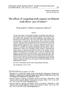
Figure 3: Trade Shares of Major Exporting Countries of Motor Vehicle Parts: The French Market

INFORUM

11

September 1994

Figure 4: Trade Shares of Major Exporting Countries of Motor Vehicle Parts: The German Market

INFORUM

12

September 1994

Figure 5: Trade Shares of Major Exporting Countries of Motor Vehicle Parts: The Italian Market

INFORUM

13

September 1994

Figure 6: Trade Shares of Major Exporting Countries of Motor Vehicle Parts: The Spanish Market

INFORUM

14

September 1994

In Figures 1-6, we plotted trade shares of major exporting countries of motor vehicle parts in each of the following six markets: the U.S., Germany, Japan, France, Italy and Spain. These interesting graphs reveal an important fact, namely, trade shares are not constant over time. Hence, one of the central tasks of the bilateral trade model will be forecasting the trade share matrices.

2c. Data Sources and Data Organization The main data source for historical trade flows matrices is the bilateral trade data tapes prepared by the OECD for its 23 member countries and the former Yugoslavia. For each of the OECD countries, data on imports and exports with nearly 200 trading partners worldwide are available by complete 5-digit SITC in both quantities and values at current dollar prices. There are over 3000 products defined in the 5-digit SITC, Revision III, nearly 2000 products in Revision II, and about 1400 products in Revision I. The data include both manufactured and non-manufactured products. The level of detail is sufficient for one to create trade flows matrices for products ranging from cotton to copper to computers. The OECD data are supplemented with bilateral trade data from the UN for three Non-OECD countries for which active models exist: Korea, Mexico and China. It has been nearly two years since we first started building this data bank shown above. Half of the time, however, was spent obtaining the data tapes and reading them into our computer. The OECD charges $2,500 per year for the data, while the UN sells the data at $4 per 1000 data points, or about $30 per country per year. While the high cost of data prevented us from obtaining these data from the OECD directly, INFORUM was able to acquire, at a much more conservative price, 14 years of OECD trade data (1974-86) from a Californian consulting firm which was going out of business. For data covering the more recent period (1987-91), INFORUM obtained them in the form of a "right to use" from the U.S. Treasury Department, with which we will share the trade data bank. Finally, the UN data for Korea, China and Mexico were purchased directly from the UN. The data organization that followed consists of six major steps. First, the data came on over 200 OECD and UN computer data tapes. On average, each year of the OECD trade data was written on twelve computer tapes -- six of export data and six of import data, and on each tape, a country’s trade was arranged by 5-digit SITC commodity and within the commodity it was arranged by trading partner. The UN trade data for Mexico, South Korea and China came on two tapes, and each data tape was basically organized like the OECD tapes, although format differences still exist. Table 6. Major Steps Involved in Building the Trade Data Bank Step 1: Download the Trade Data into the Computer; Step 2: Aggregate Trading Partners from 200 to about 60; Step 3: Eliminate Alphanumeric SITC codes in the Data; Step 4: Create Conversion Tables Between Various SITC Revisions and a Uniform 120 Sectors; Step 5: Convert Product Classes from 3000 to 120; Step 6: Build INFORUM World Trade Matrices.

Downloading these data required hundreds of megabytes in computer disk space and several weeks of time. After reading each of these tapes, the data consisted of bilateral flows in complete 5-digit SITC

INFORUM

15

September 1994

among the nearly 30 source countries and about 200 trading partner countries that made up the entire world. In Step 2, we reduced the number of trading partner countries by geographic aggregation from 200 to about 60 (again, see Table 2). Step 3 dealt with the elimination of the alphanumeric SITC codes in the data. There were two kinds of alphanumeric SITC codes in the OECD data. First, the OECD introduced a letter "B" at the position where the national code differed from the SITC description. For example, on data from Austria, the OECD listed all commodities of group 251 ("Pulp and waste paper") not available separately under code 251BB. Second, to retain confidentiality in all or part of the SITC at detailed levels, and the divulgence of trade at higher levels by origin or destination, the OECD gave complete data, including a complete geographic breakdown, only at the less detailed level of the SITC. The statistics were treated by a program which subtracted the confidential data given at a more detailed level in the same class. The remainder was recorded on the tape in an alphanumeric codification ending in one to four letters "A". For example, a reporting country provided the OECD with data from division 51 ("Organic chemicals") with complete geographic breakdown. These data were treated and recorded on the tape under the code 51AAA. In adding up the data recorded under 51AAA and all other data under headings beginning with 51, the total equals that of division 51 as provided by the reporting country. When the reporting country provided total value without a complete geographic breakdown at a detailed level, the difference was recorded under the geographic code "secret" under number 8210. Table 7 illustrates this process. In this Table, the data given under code 51 were obtained by the Table 7: An Illustration of Alphanumeric SITC Codes in the OECD Trade Data SITC 51 512 513 514 515 51A REVISED _______________________________________________________________________________________ A B C D E F = A(B+C+D+E) PARTNER by program COUNTRY __________________________________________________________________________________________ Total 596 439 88 56 1 12 XXXA 149 XXXB 69 XXXC 44 XXXD 45 XXXE 17 XXXF 76 Other Nations 196 8210 (secret) 0

92 48 29 26 12 58 99 75

28 16 5 2 0 11 12 14

21 3 2 3 0 3 21 3

0 0 0 0 0 0 0 1

8 2 8 14 5 4 64 -93

OECD from the reporting country with a complete geographic breakdown. Data for groups 512, 513, 514 and 515 which made up division 51 were calculated from the 5-digit SITC level, as given by the reporting

INFORUM

16

September 1994

country. For some of the 5-digit positions, the reporting country has given only the total trade, and this is then registered under "secret" code 8210. The data recorded under heading 51A on the tape were thereafter obtained by subtraction. It should be noted that: a) For a given product at 4- or 5-digit level, the reporting country has maintained confidentiality. Non-disclosed trade was included with a complete geographic classification in the data of division .15 The total of this undisclosed trade was +12. b) The total amount in division 51 under code 8210 was zero. Given that the sum of the data recorded under geographic code 8210 for SITC headings 512, 513, 514, 515 and 51A must be zero, the program placed a negative number in the column 51A for geographic code 8210. This negative number was equal in absolute value to the sum of the figures under code 8210 in columns 512, 513, 514 and 515. The present of alphanumeric SITC codes in the OECD trade data was of concern to us because the sectoring plan of the bilateral trade model required us to aggregate the data in complete 5-digit SITC codes to the 120 product classes. Since, for instance, not all 5-digit SITC data under division 51 fell under the same trade model sector, we needed to know where to place data under 51A. The only way to accomplish this, it seemed to us, was to reallocate the data under 51A back into the nonalphanumeric 5-digit SITC codes, namely, 512, 513, 514 and 515, for there was clear correspondence between these non-alphanumeric 5-digit SITC codes and the 120 trade model sectors. As it turned out, the reallocation of data in alphanumeric SITC codes ending with letters "A" presented us a well-defined rAs problem. Well-defined because row sums and columns could be easily established, and the matrix to be controlled could also be easily constructed, with the 5-digit commodity codes across the top of the column and trading partners down the side. The rAs procedure then would be able to eliminate the alphanumeric code 51A and the "secret" trading partner 8210, without altering the total value of the data under heading 51. For alphanumeric codes ending with letters "B", a reporting country’s data were directly distributed to its respective trading partners according to the share of each non-alphanumeric 5-digit SITC code under the same heading. It should be noted that alphanumeric product codes appeared in the data of nearly all reporting OECD countries throughout the 1974-91 period. Because of the pervasiveness of the alphanumeric product codes, the elimination of them took more than a month of intense work. In Step 4, we worked on creating conversion tables between 5-digit SITC codes and the 120 trade model sectors. For most of the 1970’s, all OECD countries reported the trade data in SITC, Revision I. Then starting in 1978, most OECD countries began to report the data in SITC, Revision II. And in 1988, nearly every country switched again, reporting the data in SITC, Revision III. Obviously, separate conversion tables were necessary to convert the data in different revisions of SITC into the 120 sectors of the bilateral trade model. It should be pointed out that there was no one-to-one conversion from the commodity classification (SITC) into the 120 trade model sectors. There are essentially two ways of dealing with the problem: assigning each multi-industry commodity entirely to the single industry code judged to be most appropriate, or splitting them among all the relevant industries. The second solution has been adopted by the Economics and Statistics Department of OECD,

INFORUM

17

September 1994

the United Nations Statistical Office and the World Bank, who jointly developed a set of conversion tables. Two of these tables translate SITC Revision I and Revision II to about 80 International Standard Industry Classification (ISIC) codes for manufacturing sectors, while the third table converts SITC Revision III back to SITC Revision II, thus providing an indirect link between SITC Revision III and ISIC codes. The gist of the first two conversion tables is that they distributes each multi-industry 5-digit SITC commodity among the relevant 4-digit ISIC codes according to the industrial composition of trade by Common Market countries in 1975. These conversion tables, however, can be criticized because it applies the same fixed allocation factors for all years and to trade by all countries (including non-EEC Members). While the second method is clearly unsatisfactory, it nevertheless appears preferable to the alternative approach of allocating multi-industry commodities in their entirety to the single most appropriate industry. Fortunately, only a few SITC codes are multi-industry, and most commodities can be unambiguously allocated to ISIC industries. Our own conversion tables are based on these OECD tables. For the purpose of this study, we modified these tables to include non-manufacturing industries and to add further breakdowns in some of the manufacturing sectors. The end results, capping off months of meticulous mapping of different commodity codes, were a set of three tables which were used to convert three different revisions of SITC codes into a unified classification of 120 commodity categories, which was carried out in Step 5. At this point, the INFORUM World Trade Data Bank (a G bank) was born. In Step 6, we created historical trade flows matrices for the 16 countries and regions in a VAM bank. Here we were faced with the perennial problem that the data for country A’s exports of product i to country B were not the same as country B’s imports of i from country A. Errors due to differences of concept, differences in valuation, timing gaps (recording of imports happens later than recording of exports), differences in methods of calculation, exports of ships to open-registry countries, etc. all contributed to the discrepancy. Fundamentally, we have relied upon the import statistics, which is based on the understanding that import data tend to identify the origin better than export data identify the destination, largely because imports loom larger in the collection of customs revenue (Maskus, 1989). Specifically, the import data of the 28 source countries were used to fill the first 14 columns. In the last column, imports of the rest of the world from each of the 13 countries and one region were derived from the corresponding export data of these countries and regions. It should be noted that these matrices are not "closed", in the sense that the intraregional trade flows between the ROW and the ROW are absent. Presumably, these flows can be determined from the residuals between the total imports of the 16 countries and regions and the total world imports by commodity. However, we do not have any data on total world imports. The closest source is total world imports in the UN’s International Trade Statistics Yearbook, but the data are not published at the 5-digit SITC level. Furthermore, these data are not true "total world imports", because, according to the UN, they account for only about 75% of the total world imports. In addition, we are told by the UN, acquiring these data for a number of years on computer tapes will be very "expensive". So for now, these trade matrices remain "open".

3. Estimating Trade Share Functions: The Methodology The next task in building the bilateral trade model is to formulate and estimate the trade share functions. In general, movements in international trade shares may be attributable to a wide range of complicated factors: price competitiveness, changes in tastes, habits, and governmental actions on subsidies

INFORUM

18

September 1994

and quotas, export promotion efforts, product range, quality changes of product, after-sales service, domestic supply constraints, etc. As practical model builders, however, we cannot formulate the forecasting equations as if we were simply testing hypotheses. We want a simplified representation of the trade share function which has reasonable values of its coefficients and will respond to experiments somewhat like the real economy would. Another constraint on these forecasting share equations is that the independent variables must be available. We will rely on individual national models for the independent variables. The national sources do not, of course, have exactly the same sectoring plan as the linking trade model, so "bridges" (classification conversion schemes) have been built between them, and exchange rates will be used to make these domestic currency-based data comparable from one country to another. In our trade share functions, movements in the trade share will depend on price competitiveness, domestic demand "tightness", and a quality factor. The relationship between one country’s trade share and her price competitiveness belongs to the core of the international trade analysis, and has been the subject of many previous investigations, including our own Nyhus study in 1975. Examining bilateral trade flows during the 1962-72 period, Nyhus found that prices could only explain half of the movements in the trade shares. The case for including non-price factors in the trade share function is strong. However, many non-price factors suggested by theories are difficult to quantify. Export promotion efforts and changes in tastes and habits are good examples. Some researchers resort to a time trend variable to capture the effects of non-price factors on the trade shares. Of course, a time trend has no economic meaning. In this study, we will experiment with two non-price variables: relative domestic demand (RDD) and investment-output ratio (IOR). RDD is a ratio of an exporting country’s domestic demand relative to its output. It is a measure of an exporting country’s domestic demand "tightness". A high RDD is expected to exert an downward "pull" on its trade shares, due to less aggressive export effort on the part of the exporting country, while a low RDD may apply an upward "push" on its trade shares, mainly because of the more aggressive export drive triggered by low domestic demand. In the U.S., for instance, it has been observed that the whole machine tools industry lost all of its overseas markets at a time when the domestic demand for machine tools was running high. The second non-price variable is IOR, which is a ratio of cumulated recent investments in a given sector over its output. It is designed to help capture quality changes of product that are not reflected in the price indexes as they are reported. This has been vividly demonstrated by the rise in the share of Japan in the imports of automobiles in many countries. Apparently, recent new investment in high-quality manufacturing equipment has resulted in quality changes which do not show up in the price indexes. The basic form we expect to use for the share of country i in year t in the imports of a given product into a given country j, Sij, is

Si j t Si j 0 (

INFORUM

Pe i t bi j RDDi t ci j IORi t di j ) ( ) ( ) Pw j t RDDw j t IORw j t

19

(1)

September 1994

Here, Peit is the effective price of the good in question in country i in year t, and is defined as a weighted average of present and past domestic market prices: 2 Pe i t

τ 0

wτ Pi t

τ

(2)

Note that the distributed lag on prices w’s are assumed to vary from commodity to commodity; but for a given commodity, they are assumed to be the same for each importing country. One of the properties the trade share function should embody is homogeneity in prices. That is, if all domestic prices, Peit, are doubled then a doubling of the world prices as seen by each importing country (or its import prices) should leave the price ratio unchanged. We have attempted to build such a characteristic into the trade share function through the an implicit definition of the world prices as seen from a given importing country j, Pwjt:

i

Si j 0 (

Pe i t bi j ) 1 Pw j t

(3)

For the same reason, measures of world relative domestic demand, RDDwjt, and world investmentoutput ratio, IORwjt, have been defined below: RDDi t ci j ) 1 RDDw j t

(4)

i

Si j 0 (

IORi t di j ) 1 IORw j t

(5)

i

Si j 0 (

The estimation of b’s, c’s, d’s and w’s requires an iterative non-linear method. The non-linearity arises because these parameters enter eq. (1) both directly (in the exponents) and indirectly (through the implicit definition of the world price, world relative domestic demand, and world investment-output ratio). Beginning with initial w’s we first determine the effective price Pei from eq. (2). For the very first pass of the solution, we also compute the world price Pwj, world relative domestic demand RDDwj, and world investment-output ratio IORwj through the following 3 equations:

INFORUM

20

September 1994

Pw j t

Si j t 1 Pe i t

(6)

i

RDDw j t

Si j t 1 RDDi t

(7)

i

IORw j t

i

Si j t 1 IORi t

(8)

Then we estimate eq. (1), by regression, for b, c and d. With these parameters we solve for the world price Pwj, world relative domestic demand RDDwj and world investment-output ratio IORwj that satisfy eqs. (3-5) respectively. Finally, we conduct a constrained estimation of the distributed lag on prices w’s via eq. (1) for each importing country. Then with newly estimated w’s, b’s, c’s, and d’s we go through the entire process again. When the change from one set of w’s to the next is within our tolerance level we stop.

4. Concluding Remarks The primary purpose of this paper is to summarize the work that has been done in building a bilateral trade model for the INFORUM international system of national interindustry-macro models. We have presented two significant pieces of data work: the INFORUM World Trade Data Bank and INFORUM World Trade Matrices. While these data banks are the foundation of the bilateral trade model under construction, their usefulness certainly goes beyond the present study. We have also briefly discussed the methodology that will be used in estimating the trade share function -- a central element of the bilateral trade model. The estimation results, when completed in the coming months, will demonstrate the effects of both price and non-price factors on the movements of the trade shares. When Douglas Nyhus built the first comprehensive trade model nearly 20 years ago, most of the today’s INFORUM national models were either not yet conceived or still in the very early stage of development. While the trade model has not been updated over the last two decades, because of a lack of necessary data, the INFORUM national models have grown in number and scope. With the data banks presented here, at last, the time is ripe to bring them together with a thoroughly up-to-date link system.

INFORUM

21

September 1994

References

Armington, P.S., "A Theory of Demand for Products Distinguished by Place of Production," International Monetary Fund Staff Papers. 16: 159-176, 1969a. ______, "The Geographic Patterns of Trade and the Effects of Price Changes," International Monetary Fund Staff Papers. 16: 179-197, 1969b. Bryant, R.C. et al., Empirical Macroeconomics for Interdependent Economies. Washington D.C.: The Brookings Institution, 1988. Cline, W.R., United States External Adjustment and the World Economy. Washington, D.C.: Institute for International Economics, 1989. Fair, R.C., Specification, Estimation, and Analysis of Macroeconometric Models. Cambridge, Mass.: Harvard University Press, 1984 Italianer, A., Theory and Practice of International Trade Linkage Models. Dordrecht: Martinus Nijhoff Publishers, 1986. Magee, S.P., "Prices, Incomes and Foreign Trade," in Kenen, P.B. (ed.), International Trade and Finance: Frontiers for Research. Cambridge: Cambridge University Press, pp. 175-252, 1975. Maskus, K.E., "Comparing International Trade Data and Product and National Characteristics Data for the Analysis of Trade Models," Paper presented at the Conference on Research in Income and Wealth. Nov. 3-4, 1989, Washington, D.C. Nyhus, D.E., "The INFORUM International System," Economic Systems Research. Vol. 3, No. 1, 1991. ______, "The INFORUM-ERI International System of Macroeconomic Input-Output Models," in M. Ciaschini, ed., Input-Output Analysis: Current Developments. New York: Chapman and Hall, 1988. ______, "A Detailed Model of Bilateral Commodity Trade and the Effects of Exchange Rate Changes," in Peterson (ed.), Econometric Contribution To Public Policy. London: Macmillan, 1978. ______, The Trade Model of a Dynamic World Input-output Forecasting System. Ph.D. Thesis, University of Maryland, 1975. Rhomberg, R.R., "Possible Approaches to a Model of World Trade and Payments," International Monetary Fund Staff Papers. 17 : 1-26, 1970. ______, "Towards a General Trade Model," in Ball, R.J. (ed.), The International Linkage of National Economic Models. Amsterdam: North-Holland, 9-20, 1973. Samuelson, Lee, "A New Model of World Trade," OECD Economic Outlook, Occasional Studies, December 1973.

INFORUM

22

September 1994

Taplin, G.B, "Models of World Trade," International Monetary Fund Staff Papers. 14 : 433-455, 1967. Waelbroeck, J., "The Methodology of Linkage," in Ball, R.J. (ed.), The International Linkage of National Economic Models. Amsterdam: North-Holland, 45-61, 1973.

INFORUM

23

September 1994