Working Paper 50
B Y PA O L O A B A R C A R
The Return Motivations of Legal Permanent Migrants: Evidence from Exchange Rate Shocks and Immigrants in Australia January 2017
WORKING PAPER 50
MATHEMATICA POLICY RESEARCH
ABSTRACT
Why do legal permanent migrants return to their home countries? How do home country conditions influence such a decision? This paper uses exogenous exchange rate shocks arising from the 1997 Asian financial crisis to distinguish between whether Australian immigrants are target earners or life-cycle migrants. A 10 percent favorable shock (a depreciation in home country currency) leads to a 10 percent reduced likelihood of return in a two-year period. The effect is stronger for those with pre-existing intentions to return, weaker for those undecided, and zero for those who initially desired to stay. These results favor a life-cycle explanation for migrant behavior and reject the theory that migrants are target earners who seek to invest upon return home.
The author is especially grateful to Dean Yang for his guidance and advice. I also thank Hillel Rapoport, Raj Arunachalam, Jeff Smith, Anne Lin, Minjoon Lee, Prachi Jain, Hyejin Rho, and Evan Borkum for helpful comments and suggestions.
i
WORKING PAPER 50
I.
MATHEMATICA POLICY RESEARCH
INTRODUCTION
Many people who live and work outside their country of birth eventually return to their home country. Although official government statistics are often lacking, indirect estimates of migrants’ movements from different countries over time suggest considerable flows. Jasso and Rosenzweig (1982), for example, suggest that more than 20 percent of immigrants chose to remigrate from the United States in the 1970s. Dustmann and Weiss (2007) approximate that 40 percent of all male immigrants and 55 percent of female immigrants left the United Kingdom five years after arriving there in the 1990s. Most recently, Gibson and McKenzie (2011) find that more than a quarter of the “best and brightest” students who ever migrated from three Pacific countries ultimately ended up returning (33 percent in Tonga, 27 percent in Papua New Guinea, and 26 percent in New Zealand). The fact that migrants choose to return in seemingly substantial numbers poses a puzzle. People move to where they earn the most, at least according to traditional economic theory (Sjaastad 1962; Harris and Todaro 1970). Hence, most returns should occur when earnings in places of origin surpass those at the destination. Yet earnings in migrant-sending countries rarely overtake those of receiving countries’ earnings. There should be little or no return. Reality appears to defy this simple prediction. More nuanced theories go beyond income maximization and favor the idea of migrants’ inclination to invest or consume in their home countries. Such theories allow for marginal changes in home country conditions to matter for migrants’ behavior, even in the absence of wage level reversals. Two competing models are at the forefront, one that regards migrants as target earners and the other as life-cycle agents. As a target earner, a migrant is creditconstrained, so she works abroad until she accumulates enough savings to finance an enterprise upon returning home (Piore 1979; Mesnard); the primary motive is investment. As a life-cycle agent, a migrant weighs the marginal benefits of obtaining higher income in the host country versus the marginal costs of remaining overseas, given that consumption of goods and services in the home county is preferred (see, for instance, Stark et al. [1997] or Dustmann [2003]); the goal is to consume. The two models generate different predictions as to how migrants respond to home country factors. Most notably, a target earner is thought to cut her stay abroad shorter when her purchasing power for the home country increases, while a life-cycle migrant prolongs her stay abroad. Empirical investigations into why migrants return to their home country have been scant and limited to particular contexts. Governments seldom record the flow of migrants, let alone track their location over time. Another issue is the difficulty of isolating exogenous variation in factors that affect return, limiting the ability for causal inference. Most studies focus on correlations. Constant and Massey (2002), for example, examine correlations between covariates of social and economic attachments in the home country with migrant return and found that these are strongly associated for a sample of German guest workers. Kirdar (2013) demonstrates that immigrants to Germany shorten their stays overseas when purchasing power increases for their home country. A chief concern with these studies, however, lies with omitted variable bias, as source country factors are possibly endogenous to variables that are unobserved. The fact that migrants with more social attachments at home are more likely to return need not imply a causal relationship.
1
WORKING PAPER 50
MATHEMATICA POLICY RESEARCH
The group may simply possess other unmeasured characteristics related to social attachments that make return appealing. Yang (2006) perhaps comes closest to identifying the causal impact of changing home country conditions on return. To confront endogeneity, the author uses an unexpected event, the 1997 Asian financial crisis, which caused substantial and varied exchange rate shocks between the Philippine peso and foreign currencies. Filipino migrants work in a diverse set of countries abroad, so the crisis created a situation in which as if each migrant were randomly allocated different exchange rate shocks during this period. By comparing the behaviors of Filipino migrants who attained greater and smaller shocks, the study establishes the causal impact of changing exchange rates on migrants’ decisions to return home. Filipino migrants appear to be driven by life-cycle considerations. They prolong their stay abroad when they experience favorable changes to their purchasing power at home. This paper focuses on Australia’s permanent immigrants and their motivations for return. Employing a strategy similar to Yang’s (2006), I use exchange rate shocks brought about by the Asian financial crisis, but look at a mirror image: data from a destination country on immigrants from multiple origin countries. Doing so provides several new insights that complement previous research: First, because the source of variation is in places of origin rather than destination, I am able to distinguish the effects of exchange rate shocks from those of other home country shocks that may also influence return, such as changes in home country gross domestic product (GDP) and unemployment. Second, I capture households whose members have all migrated and otherwise would have been absent in data collected from the home country, a limitation of Yang (2006). Third, I am able to test which theory of migration likely holds for legal permanent migrants. Whereas Yang (2006) focused primarily on Filipino migrants in temporary work contracts abroad, it is unclear whether his results must hold for other types of migrants as well, such as those granted permission for indefinite stay at the destination. For that set of individuals, a reasonable prior in fact is that there could be no motivation for return at all. Australia is a natural setting for studying migration because of its large immigrant community; 24.7 percent of its population is foreign-born. Most immigrants are legal permanent residents (as opposed to undocumented) whose immediate relatives are already present in the host country. My main contribution is the finding that a 10 percent depreciation of home country currency—which on average was what countries in the sample experienced over the two-year study period—leads to a 0.37 percentage point reduction in the probability that a migrant will return to her home country. The two-year permanent return rate in the study period was 4.1 percent, so the effect is equivalent to almost 10 percent of the return rate. The result is robust and consistent with the story that migrants return because of life-cycle considerations. The effect is strongest for migrants who have predetermined that they want to return, weak for those initially undecided, and null for those who originally stated their desire to stay. This is evidence that migrants seek to optimally time their return, rather than to decide whether to return, on the basis of favorable conditions. Moreover, this study offers evidence that the effect of the exchange rate shocks is not merely a proxy for the influence of other macroeconomic conditions such as GDP per capita growth or the change in unemployment in the home country. Rather, evidence
2
WORKING PAPER 50
MATHEMATICA POLICY RESEARCH
suggests that return is a function more of purchasing power and consumption than employment possibilities in the origin country. Migrant-sending countries often lament losing highly skilled nationals to richer countries through international migration, whereas return is often seen as the reverse, as migrants bring back essential human capital. With governments keen on enacting policies that encourage return, distinguishing between the motivations of legal permanent migrants is crucial to understanding how best to motivate migrants to return and their potential effects on the economy. II. THE ASIAN FINANCIAL CRISIS OF 1997 AND ITS IMPACT ON AUSTRALIA
Although few observers had hinted at the possibility of a crash,1 the crisis that eventually beset the booming East and Southeast Asian economies of the 1990s is widely regarded to have been unexpected. Telltale signs were absent: Savings rates were high, inflation was low, and fiscal accounts were balanced (Radelet and Sachs 1998). Credit agencies such as Standard and Poor’s and Moody’s provided no indication of changing risk in country ratings until after the crisis had begun. The Asian financial crisis is said to have started officially in July 1997, with the devaluation of the Thai baht. The event triggered a wave of capital flight from the region, as foreign investors withdrew funds, speculating on the weakness of surrounding economies. Five countries were most affected: Thailand, Indonesia, South Korea, Malaysia, and the Philippines. In the year before the crisis, inflows of foreign capital into these countries amounted to $97.1 billion. In just a year afterward, outflows were estimated to be $18.1 billion (Radelet and Sachs 1999). Hong Kong, Singapore, Taiwan, and Laos suffered considerable economic losses as well, albeit to a lesser degree. Currency devaluations followed. What economic analysts had previously dubbed the “Asian economic miracle” had come to an end. For the most part, Australia came out unscathed. Diminished regional demand for its exports was a brief concern, but although exports did subsequently decline (Gunawardana 2006), the impact on the local economy was negligible. Real GDP continued to grow by 4.0 percent during 1997–98, up from 2.8 percent in the previous period; unemployment fell from 8.7 percent to 8.3 percent; and private consumption and business investment actually rose by 4.6 percent and 11.6 percent from the previous year (Queensland Treasury and Trade 1998). Makin (1999) attributes the resilience to the switching of international capital out of Asian markets into Australasian and other markets. The flows kept interest rates low and asset values high in advanced economies. The Asian financial crisis makes for a compelling natural experiment. That Australia was relatively unaffected holds constant the local economic conditions faced by immigrants in the country at that time. But because these migrants came from a variety of backgrounds, they effectively experienced different home country shocks from the crisis. Thus, one approach to understanding what motivates return is to discern which migrants were more likely to come back by comparing the behaviors of migrants faced with different shocks. Most notable among shocks 1
See, for instance, Park (1996), who warned about the excessive influx of foreign capital into East Asia. He suggested that it was both speculative and short term and that some controls might be necessary to discourage capital movements.
3
WORKING PAPER 50
MATHEMATICA POLICY RESEARCH
were exchange rate changes that occurred between home country currencies and the Australian dollar. Migrants had their home country currencies appreciate or depreciate to varying degrees in a way that was unexpected and plausibly random. Figure 1 depicts the exchange rates during the time of the Asian financial crisis between the Australian dollar and foreign currencies of the top 15 home countries of migrants in the data. The exchange rates are expressed in foreign currency over Australian dollar (e.g., PHP/AUD) and are normalized to one in January 1996 for ease of comparison. An increase represents home currency depreciation with respect to the Australian dollar and signifies a higher purchasing power for the migrant looking to go home. A structural break in trends occurred around July 1997, the start of the crisis. Variation around this period is what this study exploits. Figure 1. Foreign exchange rates of the top 15 home countries of immigrants to Australia
Notes:
Historical exchange rate data are from Oanda Corporation. The exchange rates are expressed in foreign currency over Australian dollar (e.g., PHP/AUD) and were normalized to 1 in January 1996.
III. DATA AND DESCRIPTIVE STATISTICS
Data for this study comes from the Longitudinal Survey of Immigrants to Australia (LSIA), a nationally representative study of principal immigrant applicants issued permanent visas
4
WORKING PAPER 50
MATHEMATICA POLICY RESEARCH
offshore who arrived in Australia between 1993 and 1995.2,3 The survey was conducted in three waves of interviews, and the focus in this study is on the second and third waves, implemented from 1995 to 1997 and 1997 to 1999, respectively. This nicely corresponds to the years before and after the Asian financial crisis. The main sample for this study thus consists of 3,069 principal immigrants, 15 to 60 years old, who have identifiable countries of birth and historical exchange rate data available for their origin countries. Information on whether these individuals returned to their home country is captured by an attrition indicator, which was recorded by LSIA enumerators. As part of its migration program, the Australian government allocates permanent visas under five broad categories: preferential family, concessional family, business skills and employer nomination scheme, independent, and humanitarian. The labor market has always played a crucial role in this structure. Applicants under the independent and concessional family streams are subject to a points test in which they are allocated points as they satisfy criteria deemed in demand by the labor market (such as age, education, experience, and English language ability); visa eligibility is determined by their passing a predetermined threshold of points. The employer nomination scheme is reserved for firms sponsoring workers. Business skills visas are granted for entrepreneurs who invest a certain amount of capital in the country. The preferential family and humanitarian visa streams are the only categories that do not depend on economic circumstances. The former is reserved for close relatives of Australian citizens or permanent residents, the latter are for refugees and their family members. The number of visas issued per year is capped. For 1993–1994, the total number granted for all streams was 76,870 (Phillips et al. 2010). Table 1 shows the resulting composition of immigrants in the main sample. According to the LSIA, immigrants to Australia are typically young (age 33), married, and well-educated (42 percent had at least a bachelor’s degree). They obtain legal residence most commonly through family sponsorship, and they arrive initially with a significant amount of funds (more than 25,000 AUD, on average). A majority declare typical household members to be present with them in Australia after two years of migration. Sixty percent of households do not have members remaining in their home countries. The number increases to 71 percent when considering oonly close relatives (spouse, son, or daughter). Only 19 percent sent money to relatives or friends overseas during the previous two years. Immigrants to Australia come from a diverse set of countries. Table 2 presents a tabulation of individuals from the top 15 source countries in the sample. England is the primary source, with 281 individuals, but countries are fairly evenly represented. Asian countries most affected by the 1997 crisis (Indonesia, South Korea, Thailand, Malaysia, and the Philippines) take up a considerable share of the sample.
2
The source of the data is the Department of Immigration and Citizenship of the Australian Government. Available at http://www.immi.gov.au/media/research/lsia/lsia01.htm#x1. 3
The survey excluded New Zealanders, who comprise the majority of immigrant inflows to Australia.
5
WORKING PAPER 50
Table 1.
MATHEMATICA POLICY RESEARCH
Descriptive statistics for the sample of immigrants Standard deviation
Minimum
Maximum
8.59
15
60
3.53
1.85
1
14
0.60 0.27 0.13 26,332
94,439
0
1,100,000
0.20 0.29 $11,353
0.00 −0.29 $472
1.00 3.10 $67,170
Mean Panel A: Immigrant characteristics (N=3,069) Proportion male Age Married Highest formal qualification Higher degree Post graduate diploma Bachelor’s degree Technical/professional qualification Trade 12 or more years of schooling 11 or fewer years of schooling Visa classification Preferential family Concessional family Business skills & employer nomination Independent Humanitarian
0.57 32.72 0.72 0.12 0.06 0.24 0.23 0.07 0.13 0.14 0.45 0.18 0.13 0.20 0.05
Panel B: Household characteristics (N=3,069) Household size Number of household members in home country 0 1 2 or more AUD value of funds arrived with when first immigrated Average weekly incomea None $1 to $57 $58 to $96 $97 to $154 $155 to $230 $231 to $308 $309 to $385 $386 to $481 $482 to $577 $578 to $673 $674 to $769 $770 to $961 $962 or more Household sent money overseas to relatives/friends Place of residence New South Wales Victoria Queensland South Australia Western Australia Other
0.09 0.05 0.03 0.10 0.09 0.07 0.07 0.10 0.10 0.07 0.05 0.07 0.11 0.19 0.43 0.23 0.11 0.05 0.12 0.06
Panel C: Other Return rate Exchange rate shock (in percentage change) GDP per capita (in USD, PPP)
0.04 0.10 $13,977
6
WORKING PAPER 50
MATHEMATICA POLICY RESEARCH
Table 1 (continued) To minimize missing observations, average weekly income was constructed by taking the maximum average weekly income between the primary applicant and the spouse. This is an imperfect measure of household income, although all the following regressions are robust to using average income of only the principal applicant. Alternate measures that the LSIA provides include total household income and total weekly income from all sources, but these contain many missing observations. a
I assign migrants exchange rate shocks by calculating the change in their home country exchange rate that occurred in the period between their Wave 2 and Wave 3 interviews.4 I follow Yang (2006) in using nominal instead of real exchange rates, given that data on the former are available on a daily basis. This allows for the changes in exchange rates to be calculated precisely before and after interview dates. Daily historical exchange rates were obtained online from Oanda Corporation.5 The exchange rates are expressed in the home country currency over Australian dollars such that an increase represents a depreciation of the home currency and a decrease signifies an appreciation with respect to the Australian dollar. An increase in the exchange rate can be thought of as favorable to immigrants because it raises the foreign currency value of earnings when used for home country consumption. How were the currencies of migrants’ countries affected by the Asian financial crisis? The last column of Table 2 displays the calculation of mean exchange rate shocks experienced by migrants from origin countries from Wave 2 to Wave 3 of the survey. On average, country currencies depreciated by 10 percent with respect to the Australian dollar, but the shocks were varied. A number of countries saw their currencies appreciate. Some even experienced extreme changes, with Bulgaria’s currency depreciating by 310 percent, Turkey’s by 112 percent, and Romania’s by 98 percent. It is possible that the fluctuation in the currencies of these countries was only in part related to the Asian financial crisis, but migrants from all these countries are included in the analysis, for lack of any objective rule to exclude them. Robustness checks show that the results do not rely on their presence. The outcome variable of interest is return migration, captured by an attrition indicator, described in Table 3. Overall attrition in Wave 3 of the survey was 20 percent. Enumerators noted the reason a respondent could not be interviewed in a particular wave. If the respondent was found absent, the enumerator asked a friend or relative of the respondent most likely to know about the respondent’s whereabouts. This study uses overseas permanently as the indicator for return, under the assumption that it accurately reflects return migration. It is distinct, presumably, from overseas temporarily, which describes visits home or trips to other countries.
Specifically, I compute the average exchange rate for the year before each migrant’s interview date in Wave 2 and correspondingly for Wave 3, then calculate the percentage change between periods by subtracting log values of the former from the latter. Alternatively, computing exchange rate shocks by simply calculating the change in the exchange rates between Waves 2 and 3 on the exact day the migrants were interviewed do not change the results of the analysis. I give a likely interview date for migrants who were not interviewed in Wave 3 and thus have no actual interview date. The likely interview date is calculated as the mean interview date of the interview group that these migrants belonged to in the LSIA. 4
5
http://www.oanda.com/currency/historical-rates/ (accessed March 2013)
7
WORKING PAPER 50
MATHEMATICA POLICY RESEARCH
Table 2. The top 15 source countries with mean exchange rate changes experienced Origin country England Hong Kong China (excluding Taiwan) India Philippines South Africa United States of America Japan Lebanon Malaysia South Korea Indonesia Turkey Germany Thailand Other Total
Table 3.
Unable to track Refused Overseas temporarily
Deceased Other Interviewed
281 187 153 145 126 121 105 78 78 74 73 72 72 70 63 1371 3069
9.16 6.09 4.99 4.72 4.11 3.94 3.42 2.54 2.54 2.41 2.38 2.35 2.35 2.28 2.05 44.67 100.00
Percentage, cumulative 9.16 15.25 20.23 24.94 29.06 33.01 36.43 38.97 41.51 43.92 46.30 48.65 53.27 55.33 57.25 100.00 100.00
Mean exchange rate change -0.08 -0.05 -0.07 0.08 0.14 0.18 -0.04 0.16 -0.10 0.14 0.24 0.72 1.12 0.08 0.20 0.08 0.10
Reasons for sample attrition
Reason
Overseas permanently Out of scope
Percentage of sample
Sample size
Description Address information not current or inadequate. Migrant was not contacted and current location unknown. Migrant refused interview. Information given that migrant has left Australia for the scheduled interview period, but intends to return to Australia. Information given that migrant has left Australia and does not intend to return. Migrant settled in area too distant from capital city to be economically viable to interview. Migrant was deceased. Migrant too sick to interview, other reasons. Migrant was interviewed.
Total
Frequency
Percentage of sample
184
6.00
65 176
2.12 5.73
130
4.24
19
0.62
1 28 2,466
0.03 0.91 80.35
3,069
100.00
Measuring return migration in this manner makes the analysis susceptible to measurement error. For instance, overseas permanently could mean that the migrant moved to another country overseas instead of back to the home country. This paper later discusses the implications of such threats and presents robustness checks to verify that results are insensitive to relaxing such measurement error assumptions.
8
WORKING PAPER 50
MATHEMATICA POLICY RESEARCH
IV. EMPIRICAL RESULTS
The main equation to estimate is as follows: 𝑅𝐸𝑇𝑈𝑅𝑁𝑖𝑐 = 𝛼 + 𝛽1 Δ𝑙𝑛𝐸𝑅𝐴𝑇𝐸𝑖𝑐 + 𝛽3 Δ𝑌𝐸𝐴𝑅𝑆𝑖𝑐 + 𝛽4 𝑌𝐸𝐴𝑅𝑖𝑐 + 𝜀𝑖𝑐
(1)
where 𝑅𝐸𝑇𝑈𝑅𝑁𝑖𝑐 is a dummy indicating whether migrant i from country c returned between Waves 2 and 3, and Δ𝑙𝑛𝐸𝑅𝐴𝑇𝐸𝑖𝑐 is the percentage change in the home country exchange rate between interviews. 𝛽1 is the coefficient of interest, indicating the effect of a 1 percent increase in exchange rates on the probability of return. The number of years between interviews, although commonly two, varied for each migrant, and Δ𝑌𝐸𝐴𝑅𝑆𝑖𝑐 includes this number for each migrant in the equation. 𝑌𝐸𝐴𝑅𝑖𝑐 are year dummies, indicating when the interview for Wave 2 was conducted for migrant i. It stands for 1995, 1996, or 1997 and allows for time trends in migrant return. 𝜀𝑖𝑐 is the disturbance term, assumed to be uncorrelated with Δ𝑙𝑛𝐸𝑅𝐴𝑇𝐸𝑖𝑐 . Standard errors are clustered at the country level to allow 𝜀𝑖𝑐 to be correlated between individuals interviewed at the same time who are from the same origin country. Potential omitted variables might still be a concern in estimating this equation. In particular, certain migrant households might have been differentially affected by the Asian financial crisis in a way that is correlated with both their exchange rate shock and their return. This is a violation of the exogeneity assumption and biases the estimate of 𝛽1. Hence, I estimate an augmented equation (2) that includes 𝑿𝒊𝒄 , a vector of controls for migrant and household characteristics recorded precrisis for each individual (Panel A and B of Table 1 show the list of covariates). Also included are country-of-origin variables that incorporate information on common language and colonial relationship with Australia, distance from Sydney, GDP per capita, and indicators for whether the country is included in the list of those hardest hit by the Asian financial crisis.6 (2)
𝑅𝐸𝑇𝑈𝑅𝑁𝑖𝑐 = 𝛼 + 𝛽1 Δ𝑙𝑛𝐸𝑅𝐴𝑇𝐸𝑖𝑐 + 𝛽3 Δ𝑌𝐸𝐴𝑅𝑆𝑖𝑐 + 𝛽4 𝑌𝐸𝐴𝑅𝑖𝑐 + 𝜷𝟓 𝑿𝒊𝒄 + 𝜀𝑖𝑐
If Δ𝑙𝑛𝐸𝑅𝐴𝑇𝐸𝑖𝑐 is exogenous, then the estimate of 𝛽1 should be unaltered by the addition of controls. To the extent that these controls also help explain return migration, their inclusion should make estimates of 𝛽1 more precise. Main result
In Table 4, I present estimates of 𝛽1 with regressions that use OLS.7 The first column begins with a specification that excludes control variables but progressively introduces a set of countryof-origin, household, and migrant characteristics as covariates. The exchange rate shocks are negatively related to the probability of return. Column 2 includes the log of GDP per capita of the migrant’s origin country as a control; the estimated impact diminishes but remains negative 6
Data on common language, colonial history, and distance were taken from the GeoDist database (Centre d'Études Prospectives et d'Informations Internationales 2013). GDP per capita data are from the World Development Indicators of the World Bank, http://data.worldbank.org/data-catalog/world-development-indicators (accessed on July 5, 2013). 7
Probit results are similar to those of OLS and indicate statistically significant estimates in the same direction and for the same variables in all regressions in the paper.
9
WORKING PAPER 50
MATHEMATICA POLICY RESEARCH
and statistically significant. It turns out that the log of GDP per capita is an important control variable, because migrants from richer countries were more likely to return but also experienced more negative exchange rate shocks (i.e., appreciation in their currencies) during the financial crisis than those from poorer countries.8 Accounting for this, however, does not completely overturn the result. The negative estimate remains robust to including a host of additional controls on country-of-origin, household, and migrant characteristics in columns 3, 4, and 5. There is no evidence that certain types of individuals or households were impacted differentially by the financial crisis in Australia in a way that is correlated with the exchange rate shocks they experienced. Table 4.
The effect of exchange rate shocks on permanent return migration
ΔlnERATE
(1)
(2)
(3)
(4)
(5)
−0.0512*** (0.0128)
−0.0380*** (0.0095)
−0.0366*** (0.0109)
−0.0389*** (0.0099)
−0.0373*** (0.0104)
0.0172*** (0.0032)
0.0161*** (0.0034)
0.0139*** (0.0040)
0.0155*** (0.0044)
N N N 3069 0.016
Y N N 3069 0.016
Y Y N 3069 0.027
Y Y Y 3069 0.028
ln(GDP per capita of origin country) Other country-of-origin controls Household controls Individual migrant controls N R2
N N N 3069 0.007
The dependent variable is a dummy variable indicating that the individual is reported to be “overseas permanently” (assumed here to have returned to country of origin). Exchange rates are in terms of foreign currency per Australian dollar. Country-of-origin controls include indicators for common language and colonial relationship with Australia, the log distance from Australia, and whether the country was one of the hardest hit by the Asian financial crisis. Household and immigrant controls include age, sex, highest educational attainment, household size, marital status, type of visa upon admission, state of residence, average weekly income, and Australian dollar value of funds arrived with when first immigrated. Robust standard errors in parentheses, clustered at the country-of-origin level *** Significant at the 1 percent level. ** Significant at the 5 percent level. * Significant at the 10 percent level. Notes:
A 10 percent increase in the exchange rate leads to a 0.37 percentage point decline in the probability that a migrant returns. This is not trivial, provided that a standard deviation change in the exchange rate during the period was 0.29 and the permanent return rate was 4.1 percent. The effect accounts for almost 10 percent of the return rate. Legal permanent migrants remain sensitive to home country conditions. As the value of their foreign wages and savings increases with respect to home country currencies, they stay longer at the destination. Hence, life-cycle considerations appear to dominate target-earning motives. Yang (2006) finds the same to be true in his sample of overseas Filipino migrants, mostly temporary contract workers abroad with family members remaining behind. That this effect generally holds for a sample of migrants in Australia is a new finding. These individuals have permanent residence status and hold the option to stay, but they remain influenced by home country considerations.
8
The correlation between ΔlnERATE and ln(GDP per capita) is −0.18.
10
WORKING PAPER 50
MATHEMATICA POLICY RESEARCH
Differential effects by intention to return
Next I investigate whether the effect of the exchange rate shocks varies depending on the subgroup considered. LSIA enumerators asked individuals at baseline, before the crisis, whether they intended to return to their home countries sometime in the future. Possible answers included “yes,” “no,” and “not sure.” I look at whether the exchange rate shocks had varying impacts between individuals with different answers to this question. To do this, I re-estimate equation (2) with interaction terms for intention to return and the exchange rate shocks. Table 5 below presents the results with different specifications that include or leave out certain controls, while always controlling for country-of-origin variables, including log GDP per capita, which has been found to be important. Migrants who stated no intention to return are the reference group. Table 5.
The effects of exchange rate shocks by intention of return (1)
(2)
(3)
Intend to return=NOT SURE
0.0555*** (0.0104)
0.0502*** (0.0106)
0.0501*** (0.0103)
Intend to return=YES
0.1780*** (0.0433)
0.1720*** (0.0429)
0.1690*** (0.0425)
ΔlnERATE
−0.0119 (0.0106)
−0.0151 (0.00942)
−0.0130 (0.0157)
(ΔlnERATE)*(Intend to return=NOT SURE)
−0.0625*** (0.0172)
−0.0551*** (0.0175)
−0.0568*** (0.0184)
(ΔlnERATE)*(Intend to return=YES)
−0.2330*** (0.0757)
−0.2250*** (0.0747)
−0.2240*** (0.0748)
Y N N 3069 0.050
Y Y N 3069 0.057
Y Y Y 3069 0.057
Country-of-origin controls Household controls Individual migrant controls N R2
The dependent variable is a dummy variable indicating that the individual is reported to be “overseas permanently” (assumed here to have returned to country of origin). Intend to return is an indicator variable that captures the immigrant’s response to the question in Wave 2: “Do you intend to return to your home country?” Possible answers were “yes,” “no,” and “not sure.” Exchange rates are in terms of foreign currency per Australian dollar. Country-of-origin controls include indicators for common language and colonial relationship with Australia, the log distance from Australia, and whether the country was one of the hardest hit by the Asian financial crisis. Household and immigrant controls include age, sex, highest educational attainment, household size, marital status, type of visa upon admission, state of residence, average weekly income, and Australian dollar value of funds arrived with when first immigrated. Robust standard errors in parentheses, clustered at the country-of-origin level. *** Significant at the 1 percent level. ** Significant at the 5 percent level. * Significant at the 10 percent level. Notes:
As expected, those who were unsure or stated their desire to return at the onset are more likely to return in Wave 3, as opposed to those who said they did not want to return. I cannot reject the null hypothesis that changing exchange rates had no effect on those who had no plans to return. On the other hand, exchange rate shocks favorable to migrants seem to have considerably delayed the return of those who initially expressed a desire to do so. Thus, the exchange rate shocks seem to operate mostly at the level of changing the timing of return and
11
WORKING PAPER 50
MATHEMATICA POLICY RESEARCH
less on the decision to return. But action at the extensive margin also exists, at least for the undecided. A favorable shock reduces the probability of return for migrants who were unsure of return at the beginning, albeit to a lesser degree. In regressions not shown, I further investigate differential effects of the exchange rate shocks by a migrant’s pre-crisis income level and country-of-origin GDP per capita. The coefficient estimates turn imprecise but generally show that increases in exchange rates accompanied a reduced likelihood of return for all income categories and country-of-origin GDP per capita. Are exchange rate shocks merely a proxy for other macroeconomic variables?
A concern about the previous regressions might be that the exchange rate shocks merely stood as proxy for other macroeconomic shocks that occurred simultaneously in home countries during the financial crisis. In other words, given that exchange rate changes are potentially correlated with variation in GDP per capita growth, unemployment, or prices, it could be these variables that were influencing return and not the higher purchasing power resulting from the exchange rates. A direct test then would be to include these macroeconomic variables in estimating the main regression equations and observe whether the estimated impact of the exchange rate changes. Table 6 displays the results of implementing such an analysis, including GDP per capita growth and changes in unemployment in the home country between Waves 2 and 3. Table 7 does the same for prices, as computed from the consumer price index.9 Only observations without missing values are used in all indicators to hold the sample constant across regressions. The main result is insensitive to the inclusion of changes in GDP per capita or unemployment, as shown in Table 6. Column 1 replicates the main regression for the smaller sample. As shown in column 2, higher GDP per capita growth in the home country appears to increase the likelihood that migrants return, but this effect disappears once the exchange rate shock is accounted for (columns 4 and 6). Home country unemployment is found to be unrelated to return (column 3). No matter how one includes other macroeconomic variables considered here as controls, the effect of the exchange rate shocks is robust.
9
Because data on GDP per capita, unemployment, and the consumer price index were provided only as yearly averages, I could not compute the change in these variables that occurred exactly between interview dates for the migrants, in the same way I did for the exchange rate for which daily data was available. I settled for using a weighted measure in calculating the changes for these variables. For instance, if a migrant was interviewed on March 1995 for the second Wave, I assigned her country’s GDP per capita on that date as one-quarter the value of the measure for that year’s plus three-quarters the value of the previous year’s. I then did the same for the third wave interview. The resulting change in GDP per capita was the log difference between the two waves. To be consistent, I recalculated the exchange rate shocks in the same way for these sets of regressions.
12
WORKING PAPER 50
MATHEMATICA POLICY RESEARCH
Table 6. Are the exchange rate shocks merely capturing the effect of GDP per capita growth and changes in unemployment in home countries? (1) ΔlnERATE
(2)
(3)
−0.0483*** (0.0124)
ΔlnGDPPCAPITA
−0.0440*** (0.0114) 0.1750* (0.0995) −0.0024 (0.0025)
Y Y Y 2480 0.037
(5) −0.0469*** (0.0120)
0.0928 (0.0966)
ΔUNEMPLOYMENT Country-of-origin controls Household controls Individual migrant controls N R2
(4)
Y Y Y 2480 0.036
Y Y Y 2480 0.032
−0.0438*** (0.0115) 0.0838 (0.0896)
−0.0013 (0.0024) Y Y Y 2480 0.037
(6)
Y Y Y 2480 0.033
−0.0005 (0.0024) Y Y Y 2480 0.033
The dependent variable is a dummy variable indicating that the individual is reported to be “overseas permanently” (assumed here to have returned to country of origin). Exchange rates are in terms of foreign currency per Australian dollar. Country-of-origin controls include indicators for common language and colonial relationship with Australia, the log distance from Australia, and whether the country was one of the hardest hit by the Asian financial crisis. Household and immigrant controls include age, sex, education level, household size, marital status, type of visa upon admission, state of residence, average weekly income in the earlier wave, and Australian dollar value of funds arrived with when first immigrated. Robust standard errors in parentheses, clustered at the country-of-origin level. *** Significant at the 1 percent level. ** Significant at the 5 percent level. * Significant at the 10 percent level. Notes:
In all regressions, exchange rate changes appear to be the most important determinant of return. Purchasing power and consumption explain migrant return better than employment opportunities and prospects at home. Neither does the main conclusion change with the inclusion of changes in the consumer price index as a variable. Table 7 shows how changes in the general price level in the home country are related to return. Column 1 is again a replication of the main result, and column 2 shows that changing prices demonstrates a similar effect on return as exchange rate shocks. Including both variables in the same regression in column 3 keeps the point estimate for the effect of the exchange rate shock unchanged, but precision is lost—it is now significant only at the 14 percent level. Including both variables reverses the sign for the effect of a price change and brings the estimate to virtually zero. I interpret this as evidence that price changes serve merely as proxies for the exchange rate shocks.10 It appears that including price changes in the regression takes away useful variation in the exchange rate while not essentially affecting the return decision, making coefficient estimates imprecise.
10
In fact, when I re-estimated this regression using a more precise measure of the exchange rate shock that occurred exactly between interview dates from Wave 2 to 3, the coefficient on the exchange rate shock was statistically significant and the same as that in column 1, even when the change in the CPI as a control was included.
13
WORKING PAPER 50
MATHEMATICA POLICY RESEARCH
Table 7. Are the exchange rate shocks merely capturing the effect of changes in the general price level in home countries? (1) ΔlnERATE
(2)
−0.0393*** (0.0103)
−0.0418 (0.0281)
ΔlnCPI Country-of-origin controls Household controls Individual migrant controls N R2
(3)
Y Y Y 3080 0.032
−0.0361*** (0.0116)
0.0031 (0.0312)
Y Y Y 3080 0.031
Y Y Y 3080 0.031
The dependent variable is a dummy variable indicating that the individual is reported to be “overseas permanently” (assumed here to have returned to country of origin). Exchange rates are in terms of foreign currency per Australian dollar. Country-of-origin controls include indicators for common language and colonial relationship with Australia, the log distance from Australia, and whether the country was one of the hardest hit by the Asian financial crisis. Household and immigrant controls include age, sex, education level, household size, marital status, type of visa upon admission, state of residence, average weekly income in the earlier wave, and Australian dollar value of funds arrived with when first immigrated. Robust standard errors in parentheses, clustered at the country-of-origin level. *** Significant at the 1 percent level. ** Significant at the 5 percent level. * Significant at the 10 percent level. Notes:
The above analyses are unlikely to fully refute the possibility that other, unobservable factors correlated with the exchange rate might also have affected return decisions. Nevertheless, given the best available aggregate data on home country economies, the evidence suggests that the shocks operated mostly through exchange rates during the crisis. V. ROBUSTNESS CHECKS
The previous analysis relies on the assumption that exchange rate shocks during the Asian financial crisis were unexpected and exogenous. If this assumption holds, then the estimates of 𝛽1 discussed above are correctly interpreted as causal effects. I have controlled for as many possible confounding factors as the data permits. This section presents additional robustness checks. Future exchange rate shocks may be systematically related to past migration trends so that the effect is merely capturing pre-existing trends. For instance, migrants who returned despite being exposed to appreciations in their home currency could simply belong to countries that, in the past, had high propensities for return. I conduct two tests to address this concern. First, I run a placebo test in which future exchange rate shocks are regressed on past return migration. Future exchange rate shocks should not systematically predict return migration in the previous period. Second, I re-estimate equation (2), adding lagged values for previous exchange rate shocks. The tests verify that the exchange rate shocks during the Asian financial crisis do not merely reflect past trends.
14
WORKING PAPER 50
MATHEMATICA POLICY RESEARCH
Table 8 presents the falsification exercise. Panel A shows the regression of the exchange rate shocks from the Asian financial crisis on the return indicator calculated from Wave 1 to Wave 2 of the survey. Panel B shows the regression of the return variable from Wave 2 to Wave 3 on future exchange rate shocks calculated from Wave 3 to two years afterward. In both cases, I cannot reject the null hypothesis that future exchange rate shocks do not predict past return. Table 8. The effect of future exchange rate shocks on permanent return migration in the prior period Panel A ΔlnERATEwave2–wave3 Return rate Country-of-origin controls Household controls Individual migrant controls N R2
Return from Wave 1 to Wave 2 −0.0057 (0.0081)
Panel B ΔlnERATEwave3–2yrs after
0.02 Y Y Y 3535 0.005
Return from Wave 2 to Wave 3 −0.0139 (0.0128) 0.04
Country-of-origin controls Household controls Individual migrant controls N R2
Y Y Y 3069 0.025
Notes:
For panel A, the dependent variable is a dummy variable indicating that the individual is reported to be “overseas permanently” for Wave 2 (assumed here to have returned to country of origin). The exchange rate change is the change from Wave 2 to Wave 3 of the survey. For panel B, the dependent variable is a dummy variable indicating that the individual is reported to be “overseas permanently” for Wave 3 (assumed here to have returned to country of origin). The sample size is naturally smaller for Waves 2–3 migrants because some had already left the survey from a previous wave. The exchange rate change is the change in the exchange rate from Wave 3 to two years after the survey. Country-of-origin controls include indicators for common language and colonial relationship with Australia, the log distance from Australia, and an indicator for whether the country was one of the hardest hit by the Asian financial crisis. Household and immigrant controls include age, sex, highest educational attainment, household size, marital status, type of visa upon admission, state of residence, average weekly income, and Australian dollar value of funds arrived with when first immigrated. Robust standard errors in parentheses, clustered at the country-of-origin level *** Significant at the 1 percent level. ** Significant at the 5 percent level. * Significant at the 10 percent level.
Table 9 presents the results of accounting for lagged exchange rate shock variables. These variables are computed using two-year changes in the exchange rate, to conform to the exchange rate shock measured between Wave 2 and 3—typically two-year changes. Column 1 provides the baseline result from Table 4 for comparison. The sample is restricted to those with observations for lagged periods of the exchange rate shock, to achieve consistency with the sample used in subsequent columns. Columns 2 and 3 include lagged variables one period before and two periods before, respectively, as regressors. The point estimate for the coefficient of ΔlnERATE is unchanged in both. Column 4 shows a regression controlling for the long-term trend in country exchange rates, specified as the change in exchange rates for the past 10 years. Column 5 displays a control for a future exchange rate shock, measured as the change two years after the last year of interview. The conclusion from the baseline result remains unchanged. These regressions show that the effect of exchange rates does not merely reflect past trends; it is contemporaneous exchange rate shocks that influence return migration. This finding validates the focus on the period before and after the Asian financial crisis. It is within this window that shifts
15
WORKING PAPER 50
MATHEMATICA POLICY RESEARCH
in the exchange rate appear to be unrelated to past trends, hence likely to be exogenous to migrants who were faced with them. Table 9.
Are the effects of the exchange rate shocks contemporaneous?
ΔlnERATE
(1)
(2)
(3)
(4)
(5)
−0.0554* (0.0280)
−0.0557* (0.0284)
−0.0554* (0.0285)
−0.0565* (0.0284)
−0.0543* (0.0292)
0.0070 (0.0494)
0.0063 (0.0499)
ΔlnERATElag1 ΔlnERATElag2
0.0057 (0.0239)
ΔlnERATElag10yr
0.0029 (0.0031)
ΔlnERATEfuture Country of origin controls Household controls Individual migrant controls N R2
0.0104 (0.0176) Y Y Y 2596 0.024
Y Y Y 2596 0.024
Y Y Y 2596 0.024
Y Y Y 2596 0.024
Y Y Y 2596 0.024
The dependent variable is a dummy variable indicating that the individual is reported to be “overseas permanently” (assumed here to have returned to country of origin). Exchange rates are in terms of foreign currency per Australian dollar. Country of origin controls include indicators for common language and colonial relationship with Australia, the log distance from Australia, and an indicator for whether the country was one of the hardest hit by the Asian financial crisis. Household and immigrant controls include age, sex, highest educational attainment, household size, marital status, type of visa upon admission, state of residence, average weekly income and Australian dollar value of funds arrived with when first immigrated. Robust standard errors in parentheses, clustered at the country-of-origin level *** Significant at the 1 percent level. ** Significant at the 5 percent level. * Significant at the 10 percent level. Notes:
A second concern is that outliers may be driving the results. Certain countries had their currencies depreciate by as much as 100 percent during the crisis, in relation to the Australian dollar. Table 10 depicts what happens to the main regression when extreme observations are systematically dropped from the data. Column 1 again shows results for the full sample. Column 2 drops the migrants from the top three countries with the most extreme currency depreciations (Bulgaria, Turkey, and Romania) and column 3 drops the top five (adding Nigeria and Venezuela). Column 4 drops migrants who obtained higher than the 99th percentile of the exchange rate shock, and columns 5 and 6 trim those above the 95th and 90th percentile, respectively.11 In all six cases, the effect of the exchange rate shock remains negative and significant, with some evidence that trimming for extreme values even magnifies the effect. Outliers appear not to be driving the result.
11
The 99th percentile exchange rate shock is 1.2, the 95th percentile is 0.73, and the 90th is 0.29.
16
WORKING PAPER 50
MATHEMATICA POLICY RESEARCH
Table 10. The effect of exchange rate shocks on permanent return migration for the trimmed sample
ΔlnERATE Country of origin controls Household controls Individual migrant controls N R2
(1)
(2)
(3)
(4)
(5)
(6)
Full sample
W/o top 3 extreme
W/o top 5 extreme
Trim 99th percentile
Trim 95th percentile
Trim 90th percentile
−0.0373*** (0.0104)
−0.0513** (0.0207)
−0.0518** (0.0231)
-0.0437*** (0.0130)
−0.0842*** (0.0272)
−0.104** (0.0414)
Y Y Y 3069 0.028
Y Y Y 2963 0.027
Y Y Y 2948 0.027
Y Y Y 3036 0.028
Y Y Y 2915 0.028
Y Y Y 2768 0.027
The dependent variable is a dummy variable indicating that the individual is reported to be “overseas permanently” (assumed here to have returned to country of origin). Exchange rates are in terms of foreign currency per Australian dollar. Country of origin controls include indicators for common language and colonial relationship with Australia, the log distance from Australia, and whether the country was one of the hardest hit by the Asian financial crisis. Household and immigrant controls include age, sex, education level, household size, marital status, type of visa upon admission, state of residence, average weekly income in the earlier wave, and Australian dollar value of funds arrived with when first immigrated. Robust standard errors in parentheses, clustered at the country-of-origin level. *** Significant at the 1 percent level. ** Significant at the 5 percent level. * Significant at the 10 percent level. Notes:
A third concern involves measurement error. The dependent variable, return, relies on information from the migrant’s friend or relative that she returned to her home country permanently. Such reports, however, could be inaccurate. Overseas permanently could reflect other reasons for attrition that the friend or relative was unaware of. The term may also capture instances of migrants moving permanently to another country or overseas for only a temporary trip. The following analysis checks for instances in which measurement error in the dependent variable introduces bias by being systematically related to the exchange rate shocks. In the analysis, overseas permanently was interpreted to mean return home, but it could also mean the migrant moved to another country permanently. To be a threat to identification, though, it must follow that permanently migrating to other countries is somehow determined by home country exchange rates. Although that possibility cannot be fully ruled out, it is improbable that it could yield the estimates that I find. First, almost 0 percent of respondents in Wave 2 said that they “expect to immigrate to another country [aside from their former country] in the future.” The response to this question is tabulated in Table 11. Dropping these individuals in the analysis had no effect on the results. Second, because the exchange rate shocks had the most effect on those who said in the baseline survey that they intended to return to their home country, it is improbable that migrants were moving elsewhere. Thus, although overseas permanently perhaps captured movement to other countries as well, this measurement error most realistically introduced itself as random noise. The fact that the regressions are still able to measure the parameter of interest with statistical significance suggests this is not a big concern.
17
WORKING PAPER 50
MATHEMATICA POLICY RESEARCH
Table 11. Expect to emigrate to another country? Frequency Yes No Not Sure [Expect to immigrate to former country]
Percentage
28 2699 213 129
0.91 87.94 6.94 4.20
Another possibility is that measurement error, arising from other reasons for sample attrition (listed in Table 3), is driving the results. It may, for instance, coincidentally happen that those who were noted as unable to track contained those who had left for home permanently, in a way that is also related to the exchange rate shocks. At the same time, migrants traveling home could systematically have been mistaken as permanent returnees when they were in fact merely visiting. There is little evidence, however, that exchange rate shocks are related to any of these other reasons for attrition. Table 12 presents such an exercise where I regress each of these other reasons for attrition on the exchange rate shock. Only out of scope appears to be predicted by the exchange rate shocks with some statistical significance and even then the association is virtually zero. Further, when the analysis is redone and the definition of return migration is expanded to include overseas temporary instead of just overseas permanently, the results are qualitatively unchanged. These results are not included in this paper but are available upon request. Table 12. The correlation between the attrition variable and the exchange rate shocks
ΔlnERATE Country of origin controls Household controls Individual migrant controls N R2
(1)
(2)
(3)
(4)
(5)
(6)
Unable to track
Refused
Overseas temporarily
Out of scope
Deceased
Other
0.0085 (0.0131)
0.0054 (0.0113)
−0.0117 (0.0170)
0.0078* (0.0047)
−0.0009 (0.0006)
0.0131 (0.0089)
Y Y Y 3069 0.022
Y Y Y 3069 0.002
Y Y Y 3069 0.013
Notes:
Y Y Y 3069 0.000
Y Y Y 3069 0.007
Y Y Y 3069 0.007
Exchange rates are presented in terms of foreign currency per Australian dollar. Country-of-origin controls include indicators for common language and colonial relationship with Australia, the log distance from Australia, and whether the country was one of the hardest hit by the Asian financial crisis. Household and immigrant controls include age, sex, education level, household size, marital status, type of visa upon admission, state of residence, average weekly income in the earlier wave, and Australian dollar value of funds arrived with when first immigrated. Robust standard errors in parentheses, clustered at the country-of-origin level. *** Significant at the 1 percent level. ** Significant at the 5 percent level. * Significant at the 10 percent level.
18
WORKING PAPER 50
MATHEMATICA POLICY RESEARCH
VI. CONCLUSION
The United Nations has estimated that more than 232 million people (around 3 percent of the world’s population) are international migrants (United Nations 2013). Economists are just starting to understand how this growing group continues to relate to the countries they are from. Remittances of these migrants to their home country remain at the center of the conversation because of their magnitude. The developing world received $435 billion in remittances from international migrants in 2014, according to estimates by the World Bank (2014). But return migration is another potentially important avenue for development that home countries stand to benefit from. It is, however, less understood. Migrant-sending countries often lament the loss of their skilled nationals because many obtain legal permanent residence in rich countries. For this reason, return migration is often viewed positively and pursued by national governments. From their work abroad, returnees theoretically make newly acquired skills, knowledge, and connections available in the domestic economy; they invest savings accumulated from overseas in the home country. But how might governments encourage return and maximize gains from such events? Effective policy depends in part on understanding precise motivations. Target earners benefit from the expansion of credit markets. For example, loans at subsidized rates hasten return and facilitate the start-up of local businesses. On the other hand, such policies may be ineffective for life-cycle migrants. If return is indeed desired, then governments might do better by identifying consumption preferences and promoting them. To my knowledge, though, the evaluation of these kinds of programs is lacking and requires additional research. This paper examined legal permanent migrants’ motivations for returning to their home country. Such individuals are well-educated and mostly have their entire families present with them abroad. Despite this, they continue to be influenced by home country factors in their decision to return home. A 10 percent decline in home country exchange rate increases the likelihood of return in a two-year period by 0.37 percentage points. This explains almost 10 percent of the return rate. The finding is comparable, yet smaller in magnitude, to what Yang (2006) uncovered as true for temporary Filipino workers abroad. In Yang’s study, exchange rate shocks accounted for 20 percent of the return rate in a 12-month period. My results support a life-cycle explanation: returnees are concerned mostly about consumption rather than investment or employment possibilities in their home country. At least for legal permanent migrants studied here, they are not, on average, target earners who wish to generate business activity when they return. Contrary to what leaders of migrant-sending countries might hope, investment may not be the main driver of return migration. Nevertheless, returning migrants’ contributions to their home countries may lie in other venues and deserve further examination. This study showed that subgroups with predetermined expectations to remigrate in the future are most responsive to exchange rate shocks, followed by those undecided. Such evidence suggests that migrants time their return to favorable conditions. Unsurprisingly, those who stated no intention of remigration before do not seem to react to exchange rate shocks at all.
19
WORKING PAPER 50
MATHEMATICA POLICY RESEARCH
Although return migration provides a peek into the economic lives of immigrants, further research is necessary for understanding what influences their economic behavior, apart from return, and how that behavior continues or ceases to be tied to home country factors. In a recent paper, Nekoei (2013) considered how the earnings and labor supply of U.S. immigrants are affected in real time by home country exchange rates. Other fruitful areas to investigate are economic decisions such as savings and expenditures that may be affected by home country shocks. The endeavor would ultimately generate a better picture of what motivates international migrants because return migration is unlikely to be decided in isolation from other equally important economic factors.
20
WORKING PAPER 50
MATHEMATICA POLICY RESEARCH
REFERENCES
Centre d'Études Prospectives et d'Informations Internationales (CEPII). “GeoDist Database.” Available at http://www.cepii.fr/anglaisgraph/bdd/distances.htm. Accessed July 5, 2013. Constant, Amelie, and Douglas S. Massey. “Return Migration by German Guestworkers: Neoclassical versus New Economic Theories.” International Migration, vol. 40, no. 4, 2002, pp. 5–38. Dustmann, Christian. “Return migration, wage differentials, and the optimal migration duration.” European Economic Review, vol. 47, no. 2, 2003, pp. 353–369. Dustmann, Christian, and Yoram Weiss. “Return Migration: Theory and Empirical Evidence from the UK.” British Journal of Industrial Relations, vol. 45, no. 2, 2007, pp. 236–256. Gibson, John, and David McKenzie. “The microeconomic determinants of emigration and return migration of the best and brightest: Evidence from the Pacific.” Journal of Development Economics, vol. 95, no. 1, 2011, pp. 18–29. Gunawardana, Pemasiri. “The Asian Currency Crisis and Australian Exports to East Asia.” Economic Analysis and Policy, vol. 35, nos. 1–2, 2006, pp. 7–90. Harris, John R., and Michael P. Todaro. “Migration, Unemployment and Development: A TwoSector Analysis.” The American Economic Review, vol. 60, no. 1, 1970, pp. 126–142. Jasso, Guillermina, and Mark R. Rosenzweig. “Estimating the Emigration Rates of Legal Immigrants Using Administrative and Survey Data: The 1971 Cohort of Immigrants to the United States.” Demography, vol. 19, no. 3, 1982, pp. 279–290. Kirdar, Murat G. “Source Country Characteristics and Immigrants’ Optimal Migration Duration Decision.” IZA Journal of Migration, vol. 2, no. 1, 2013, pp. 1–21. Makin, Tony. “The Asian Currency Crisis and the Australian Economy,” Economic Policy and Analysis, vol. 29, no. 1, 1999, pp. 77–85. Mesnard, Alice. “Temporary Migration and Capital Market Imperfections.” Oxford Economic Papers, vol. 56, no. 2, 2004, pp. 242–262. Nekoei, Arash. “Immigrants’ Labor Supply and Exchange Rate Volatility.” American Economic Journal: Applied Economics, vol. 5, no. 4, 2013, pp. 144–64. Park, Yung Chul. “East Asian Liberalization, Bubbles, and the Challenge from China.” Brookings Papers on Economic Activity, vol. 1996, no. 2, 1996, pp. 357–371. Phillips, Janet, Michael Klapdor, and Joanne Simon-Davies. “Migration to Australia since Federation: A Guide to the Statistics. Australia Parliamentary Library. Background Note. Available at http://aphnew.aph.gov.au/binaries/library/pubs/bn/sp/migrationpopulation.pdf. 2010.
21
WORKING PAPER 50
MATHEMATICA POLICY RESEARCH
Piore, Michael J. Birds of Passage: Migrant Labor and Industrial Societies. New York: Cambridge University Press, 1979. Queensland Treasury and Trade. “Annual Economic Report, 1997–1998.” Available at http://www.qgso.qld.gov.au/products/reports/annual-econ-report/annual-econ-report-199798.pdf. Accessed June 21, 2013. Radelet, Steven, and Jeffrey D. Sachs. “The East Asian Financial Crisis: Diagnosis, Remedies, Prospects.” Brookings Papers on Economic Activity, vol. 28, no. 1, 1998, pp. 1–74. Radelet, Steven, and Jeffrey D. Sachs. “What Have We Learned, So Far, From the Asian Financial Crisis?” Consulting Assistance on Economic Reform Discussion Paper No. 37. 1999. Sjaastad, Larry A. “The Costs and Returns of Human Migration.” Journal of Political Economy, vol. 70, no. 5, 1962, pp. 80–93. Stark, Oded, Christian Helmenstein, and Yury Yegorov. “Migrants’ Savings, Purchasing Power Parity, and the Optimal Duration of Migration.” International Tax and Public Finance, vol. 4, no. 3, 1997, pp. 307–324. United Nations Department of Economic and Social Affairs (Population Division). “The Number of International Migrants Worldwide Reaches 232 million.” September 2013. Available at http://esa.un.org/unmigration/documents/The_number_of_international_migrants.pdf. Accessed Jan. 31, 2015. World Bank. “Migration and Remittances: Recent Developments and Outlook.” Migration and Development Brief 23. 2014. Available at http://siteresources.worldbank.org/INTPROSPECTS/Resources/3349341288990760745/MigrationandDevelopmentBrief23.pdf. Accessed Jan. 31, 2015. World Bank. “World Development Indicators.” Available at http://data.worldbank.org/datacatalog/world-development-indicators. Accessed July 5, 2013. Yang, Dean. “Why Do Migrants Return to Poor Countries? Evidence from Philippine Migrants’ Responses to Exchange Rate Shocks.” The Review of Economics and Statistics, vol. 88, no. 4, 2006, pp. 715–735.
22
ABOUT THE SERIES
Policymakers and researchers require timely, accurate, evidence-based research as soon as it’s available. Further, statistical agencies need information about statistical techniques and survey practices that yield valid and reliable data. To meet these needs, Mathematica’s working paper series offers access to our most current work. For more information about this paper, contact Paolo Abarcar, Researcher, at
[email protected]. Suggested citation: Abarcar, Paolo. “The Return Motivations of Legal Permanent Migrants: Evidence from Exchange Rate Shocks and Immigrants in Australia.” Working Paper 50. Washington, DC: Mathematica Policy Research, January 2017.
www.mathematica-mpr.com
Improving public well-being by conducting high quality, objective research and data collection PRINCETON, NJ ■ ANN ARBOR, MI ■ CAMBRIDGE, MA ■ CHICAGO, IL ■ OAKLAND, CA ■ TUCSON, AZ ■ WASHINGTON, DC
Mathematica® is a registered trademark of Mathematica Policy Research, Inc.