THE PRICING OF MUNICIPAL BOND INDEX FUTURES THOMAS R. HAMILTON SCOTT E. HEIN TIMOTHY W. KOCH

INTRODUCTION In June 1985, the Chicago Board of Trade began trading a futures contract based on the value of the Bond Buyer Municipal Bond Index (MBI). Unlike most financial futures, the MBI futures contract is based on a portfolio of 40 different bonds that changes in composition on the I 5th and last day of each month. As such, there is no single, well-defined deliverable instrument on which to base the pricing of MBI futures. While considerable research has examined the pricing of Treasury bill. Treasury bond, and other financial futures contracts, considerably less effort has focused on pricing MBI futures. Arak, Fisher. Goodman, and Daryanani (1987) developed an arbitrage pricing model for the The comments and suggestions of K. C. Ma, Jeff Mercer, Chip Peterson, Bruce Phelps, Charles Smith, Hoi Toles, and anonymous referees are gratefully acknowledged. We also acknowledge the valuiihle research assistance of Terrante jalhert. Finally, we wish to thank Bill McLaughlin and The Bond Buyer For supplying us with the underlying municipal security prices used in this study.

• Thomas R. Hamilton is an Assistant Professor at St. Mary's University of San Antonio. • Scott E. Hein is first National Bank at Luhbock Distinguished Scholar and Chairman, Area of Finance at Texas Tech IJniversty. m Timothy W. Koch is South Carolina Bankers Association Chair of Banking at the University of South Carolina. The Journal of Futures Markets. Vol. 14, No. 5, 575-596 {1994) © 1994 by John Wiley & Sons, Inc.

CCC 0270-7314/94/050575-22

576

Hamilton, Hein, and Koch

municipal to Treasury bond futures spread which specified a theoretical upper and lower bound for the municipal contract. They viewed the MBI as a cash asset and thus did not examine the relationship between the MBI and prices on the underlying bonds, or the impact of changes in index composition. More recently, several articles in Industry Insights: Municipal Bond Index Futures and Options noted that municipal futures appear to consistently trade at a substantial discount to their theoretical value, hut provide no empirical support for this claim. Finally, Whittaker, Bowyer, and Klein (1987) examined MBI futures trading to determine whether eash market prices were affected hy the introduction of the MBI contract, but did not address any reverse price linkage. The purpose of this research is to develop a cash-and-carry pricing model for MBI futures based on prices for the underlying municipal bonds that incorporates the impact of changing index composition, and to empirically examine whether the actual MB! futures priee differs systematically from the theoretical priee.' The article offers three contributions. First, a theoretical model is developed for the MBI futures price that reflects financing and transactions costs associated with cash-and-carry trades of the underlying MBI bonds. Second, it is demonstrated that for the 22 nearby contracts expiring between September 1985 and December 1990, MBI futures are generally priced consistently according to the theoretical model. Finally, it is shown that the revision process for the MBI does not affect the pricing of MBI futures in terms of the theoretical model. The primary finding is that MBI iutures generally are priced on a cash-and-carry basis.

THE MBI FUTURES CONTRACT Cash-and-carry trading with municipal bond futures involves arbitraging the price difference between the MBI futures contract and the cumulative prices of the underlying municipal bonds. To construct the arbitrage, traders must compare the value of their futures position with the value of the bond portfolio. The MBI is based on a diversified portfolio of 40 municipal bonds representing a cross-section of the municipal market. To qualify for inclusion in the index, each bond must be rated A or higher by Moody's and/or A— or higher hy Standard and Poor's. The term component must equal at least $50 million and the bonds must be out of syndication and thus free to trade. Each bond must have a fixed For rea.s()ns discussed later, the empirical analysis tests compare actual futures prices with the theoretical upper bound and lower hound of the no-arbitrage trading range for MBI futures.

Muni Bond Index Futures

coupon payable semiannually, have a re-offering price between $95 and $105, be callable at par with 7—16 years remaining to first call, and have at least 19 years remaining until maturity. The MBI includes both general obligation and revenue bonds, as well as bonds for different geographic regions of the U.S. A potential problem with conducting the cost-of-carry arbitrage is that the bonds used to construct the MBI change frequently. On the I 5th and last day of each month. The Bund Buyer deletes bonds that no longer represent the market and adds newly issued bonds that meet the selection criteria where appropriate, to ensure that the MBI reflects current market conditions.^ From June 1985 through December 1990, tbe number of bonds deleted/added at each revision averaged 7, ranging from 0—17. Thus, on average, the composition of the MBI changed entirely every five to six revision periods. One implication is that, prior to expiration of the MBI futures, a cash-and-carry trader may have to buy and sell bonds after initiation of an MBI futures position to adequately reduce risk. Potentially high and uncertain transactions costs, in turn, may make such arbitrage unattractive. The MBI is computed each day between 1:45 PM and 2:00 PM CST.^ First, The Bund Buyer calculates an average price for each bond by obtaining price quotes from five dealer-to-dealer bond brokers, dropping the high and low quotes, and determining the mean of the remaining quotes. Second, The Bond Buyer converts the average quoted price for each bond to an index price dividing by a conversion factor. The conversion factor is determined by the Standard Securities Calculation Methods published by the Securities Industry Association. The index price is the price at which the bond would yield 8% to maturity or first call. Third, it calculates the average of the 40 index prices. Finally, it multiplies the average index price by a continuity coefficient and rounds to the nearest 1/32 to produce the MBI. The use of continuity coefficients prevents discrete jumps in the MBI when the bonds in the index portfolio change. The MBI futures contract is valued at $1000 times the MBI value with cash settlement on the eighth to last business day in March, June, September, and December. There is no deliverable instrument. The

If a scheduled revision day is not a business day, the revision is done on the immediately preceding business day. Revisions occur after the close of trading but are announced one day prior to the scheduled day. ^During futures contract settlemenl months, the MBI is also calculated from IO:4S AM to 1:00 AM each day.

577

578

Hamilton, Hein, and Koch

actual 40-bond portfolio tbat comprises the MBI at expiration is known with certainty only after the last revision. The settlement price for the MBI futures contract at expiration (Fx) is determined as: F^ = MB/;,($ 1000)

(1)

where Fx

= the daily settlement price of the futures contract, with the subscript x denoting the expiration day of the futures, and

MBIx = the MBI value at expiration. The MBI is not a commodity in itself, but represents the average of the 40 bonds' converted prices adjusted by continuity coefficient. Investors can purchase the portfolio of 40 municipal bonds, but at an agg'"egate price different from the Index value. The actual relationship between the bond portfolio price and the Index value is shown in eq. (2). 40

= ^ ^ ^

X CC,

(2)

where MBit ^ Municipal Bond Index value at time t prior to expiration, I Pit

— the Index (converted) price of each bond i in the portfolio at time t, and

CCt

= the continuity coefficient for the portfolio at time (.

The Index price for each bond is determined by dividing the actual bond price by its conversion factor. The full expression for the MBI is thus: 40

=

^Q

X CC,

(3)

where BPit = the quoted price for bond i at time (, and Cit

= the conversion factor for bond i at time t.

It is not possible to specify the MBI value as a simple fraction of the sum of the bond prices because the conversion factors differ between the 40 bonds in the portfolio. However, because the sum of the bond prices (X(=i BPit) and sum of the converted bond prices (Xi=i(SPi(Ci()) can

Muni Bond Index Futures

be determined, the weighted effect of the conversion factors (WCt) can be used to characterize the relationship. 40

(4)

The relationship between the index value and the price of the portfolio of bonds at time ( is thus: 40

MBit = '

X CCt

(5)

The sum of the bond prices, in turn, equals a multiple of the index value. 40

J^BPu = (40/CC,)MB/ X WCt

(6)

i=\

Because the futures price must equal the index value at expiration, the relationship between the future price and sum of the bond prices at expiration is: 40 X w e

." „„

Defining Z* as [(40 X WC,/CCt)l eqs. (6) and (7) suggest that arbitragers should buy or sell Z, MBI futures contracts to match the dollar value of a futures position with the actual dollar value of the underlying bond portfolio at expiration. Z, expresses the mathematical relationship, derived from the futures contract specifications, between the futures price and the value of the bond portfolio underlying the

•*Alternatively, tbe reiationsbip between the portfolio price ^i^\ be expressed as:

tPn and MBI value at time t can

40

(40/CC,)MB/, = X ' P ' ' The use of this formulation assumes that bond.s are infinitively devisable to allow a proportion of each bond to be held in the casb portfolio or tbat the investment is sufficiently large tbal the required proportion could he held in whole bonds. The total value of ihe pruportional portfoho is tbe sum of tbe index prices of tbe honds.

579

580

Hamilton, Hein, and Koch

MBI. It is not the number of futures contracts needed to establish a minimum risk hedge.^

COST-OF-CARRY MODEL FOR MBI FUTURES The cost-of-carry pricing model, first developed by Working (1949), explains the difference between futures and cash prices in terms of carrying costs associated with arbitrage trading. When the futures price exceeds the cash price plus carrying costs, arbitragers buy the cash instrument and sell futures. When the futures price falls below the cash price minus carrying costs, arbitragers buy futures and sell cash instrument. The futures price is thus determined at the margin by arbitrage trading with the theoretical futures value equal to the cash price adjusted for carrying costs. In fact, the cost and risk of going long cash bonds and short futures differ substantially from the cost and risk of shorting cash municipals and being long futures. Generally, both the cost and risk of shorting cash municipals is greater than the cost and risk from buying municipals. Consequently, there are actually two distinct arbitrage relationships that produce asymmetric bounds. The upper bound for the futures price, associated with being long the cash instruments and short futures, is based on lower carrying costs and risk than the lower bound, associated with being short the cash instruments and long futures.

The Theoretical Upper Bound In a pure arbitrage when the actual futures price exceeds the cash price plus net financing and transactions costs, traders borrow funds to finance the purchase of 40 index bonds plus transactions costs and simultaneously sell futures. At expiration, they sell the 40 index bonds, pay the financing costs, and buy back the futures contracts. Because the value of the futures equals the bond portfolio value at expiration, the arbitrage profit will equal the difference between the initial futures value and cost of bonds minus carrying costs. This series of transactions. For an evplanation of the minimum variance technique sec Bond. Thompson, and Lee (1987). For a comparison of the regression of price changes technique with other techniques to estimate d minimum risk hedge, see Witt, Schroeder. and Hayenga (1987).

Muni Bond Index Futures

labeled a long bond arbitrage, establishes a theoretical upper bound for the price of the futures contract/' Let: BPt

= sum of the 40 cash bond prices at time t,

NFCLt = expected net financing cost of the long bond position at t, and = expected transactions costs for period t to futures expiration for buying and subsequently selling the 40 index bonds from period ( to expiration. The value of the MBI futures at time t is given by the futures price times the number of futures contracts traded (Z*). This should be less than or equal to the sum of the bond prices, net iinancing costs, and transactions costs for arbitrage to be unprofitable; FPtiZ*) < BP, + NFCLi + TCLt

(8)

The expected net financing cost {NFCL,) equals the interest cost of financing the entire 40-bond portfolio and transactions costs accounting for accrued interest due, minus the tax-equivalent value of coupon interest and reinvestment income. A fixed financing rate is assumed and it is assumed that the marginal trader pays taxes at the corporate income tax rate. Capital gains taxes are not included in the calculations, helievlng that such gains and losses will have symmetrical tax implications on both sides of the arbitrage. Expected transactions costs (TCLi) equal the product of the unit charge for each in an out trade of a cash bond, the average number of bonds sold and purchased during prior revision periods, and the number of revision periods remaining until expiration. Traders know that the futures price will equal SI000 times the MBI at futures expiration. Relationship (8) would be relatively easy to implement and test if arbitragers could buy all 40 underlying bonds and hold them to expiration of the futures contract. Arbitrage is complicated by the revision process, however, because the composition of the index changes over time. A trader who initiates a position prior to the last

*'Onee the long-bond/short-futures position is established, any relative decline in the futures price will generate Further profit opportunities for arbitragers from investing excess niar^^in halances. A corresponding rise in Futures prices will produce a deficient margin and the associaled costs. The effects ot marking-to-market are not considered in this analysis. There is also a transaction cost of establishing the futures position but this is a one-time expense that is not included in the calculations.

581

582

Hamilton, Hein, and Koch

revision date does not know with certainty which bonds will be in the MBI at expiration. There are two basic approaches to handling this uncertainty. Traders could initially buy or sell the entire complement of 40 bonds, then adjust their position by buying and selling the bonds that are added and deleted, respectively, at each revision. This increases the transactions costs but reduces uncertainty concerning the composition of the bond portfolio and thus the difference in value between the portfolio and futures position at expiration. Alternatively, traders could initially select only a subsample of index bonds considered representative of the MBI and buy and hold just these securities throughout the revision process. This latter procedure lowers transaction costs but increases the likelihood that futures price changes will not closely track prices of the subsample of bonds. Such a procedure would involve greater risk and would not represent a pure arbitrage setting. The cost-of-carry model proposed here uses the first approach. Subsequent empirical analysis will contrast the implications of the cost-of-carry model with the risk-taking strategy of buying and holding only a subset of the MBI bonds. If the risk-taking strategy is used in practice, one would expect to see a larger discount of the MBI futures price relative to the theoretical value, the farther away is delivery.

The Theoretical Lower Bound Traders will undertake short bond arbitrage if the actual futures price is less than the cash bond price net of transactions and financing costs. This involves selling the 40 index bonds short and buying MBI futures. In a short sale of municipal bonds, a trader borrows bonds posting collateral equal to the price of the bonds, and receives the proceeds from the sale of bonds. When returning the borrowed bonds the trader pays any coupon payments made during the period plus a fee for use of the bonds. In a pure arbitrage, a trader borrows sufficient funds to post the collateral and cover the scheduled coupon payments, bond use fee, and transactions costs; then uses the proceeds from the short sale either to reduce the amount of funds initially borrowed or invests in interest-bearing securities. At expiration, the arbitrager buys the 40 index bonds and returns them along with applicable fees and interest, reclaims funds posted as collateral, and repays the borrowed funds plus interest.

Muni Bond Index Futures

Letting: BPSi

= proceeds from the short sale of bonds,

NFCSj

^ expected net financing cost of the short bond position at t, and

TCS,

= expected transactions costs for shorting and subsequently buying the 40 index bonds for period t through expiration,

the value of the MBI futures at time t times the number of futures contracts traded should exceed or equal the sum of the bond prices minus net financing costs and transaction costs for arbitrage to be unprofitable: FPtiZ*) > BPSi - NFCS, - TCS,

(9)

The expected net financing cost for the short bond arbitrage (NFCSt) equals the interest cost of financing the short position minus income from investing proceeds from the short sale. An arbitrager must borrow sufficient funds to post surety equal to the bonds' value plus coupons due, pay lenders of the bonds any income that would have been earned, and cover transactions costs. A fixed financing rate is assumed with a risk premium added to account for the greater risk associated with the short position.^ Arbitragers must initially locate owners who are willing to lend the 40 index bonds for a short sale, then find and buy tbe same bonds later to cover the short position. With the revision process, the series of transactions may have to be repeated for a subsample of bonds several times before expiration. This short bond position embodies considerably more risk and potentially higher transactions costs than the long bond position. In addition, net financing costs will be greater because no coupon interest is received from owning the index bonds as with the long bond arbitrage. Finally, in some cases, the short seller may not receive the full price of the bonds such that BPSt < BP,. The net effect of these positions is to establish a range within which the futures price can vary when arbitrage is not profitable. Relationships (8) and (9) suggest the following no-arbitrage trading range:

^ [ , Zt

- NFCS, - TCS,] < FP, < [BP, + NFCL, + TCL,]-^ Zt

(10) The premium equak the TED spread, or dirt'erence between the cash three-month Eurodollar rate and three-nionlh T-bill rate.

583

584

Hamilton, Hein, and Koch

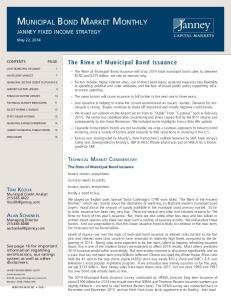
THE DATA Daily data on the MBI futures settlement price are from the Wall Street Jowmfl/for the period June 19, 1985, to December 31, 1990. Daily data are gathered also from The Bond Buyer for the same period for each of the 40 bonds included in the MBI. Unfortunately, only bid prices are available and thus the cash index is based on bid quotes. The same day futures and cash prices reflect prices at slightly different points of time, 2:00 PM versus closing CST. This means there are sampling errors in the investigation of the arbritrage linkage. The overnight repurchase agreement rate is used as the opportunity cost of funds in short-term financing to calculate expected financing costs. In the case of the short bond position, a risk premium (equal to the TED spread) is added to reflect increased risk and expense.** The transactions costs in the bond arbitrage are incorporated by assuming a $1 transaction charge for the buying or selling of bonds. EMPIRICAL RESULTS According to the cost-of-carry model, the MBI futures price should fall within the bounds given by (10). Daily values for the upper and lower bounds are calculated for the period June 19, 198S, to December 31, 1990. Figures 1—6 detail these daily bounds along witb the actual settlement MBI futures price for each of the 22 separate intervals when the contract becomes the next to deliver. Each chart illustrates the daily settlement price relative to the upper bound, based on the long bond arbitrage condition, and the lower bound, based on the short bond arbitrage condition. As transaction costs are larger the farther away is delivery, the charts show narrowing bounds as delivery approaches. The charts provide a quick means to evaluate violations of the arbitrage bounds. In particular, data for the first five nearby contracts ^Whiie there is some question as to whether the overnight RP rate is the appropriate financing rate, similar results are obtained witb the tbree-monlh Treasury bill rate as a proxy for lerm borrowing costs, Thus, the results iire virtuiilly identical regardless uF whether arbitragers finance overnight or to term. The SI charge is hased on estimates provided hy hond traders at Northern Trust in Chicago and Bear Sterns in New York who generally agree thai tbe administrative costs for each trade ticket are $tOO regardless of the number of bonds traded on the ticket, h is assumed here that an average of IOO bonds are traded on each ticket and that transactions costs are symmetric for short- and long-hond positions. If shorting bonds is more costly, the calculated lower bond will be too high witb the greatest effect near expiration.

Muni Bond Index Futures

1965 Quarter 3

July2S, 1SS5

AuotMl29.

Legend Upper Bound Settle Lower Bound FIGURE 1 1985 MBI pricf behavior.

show much more evidence of violations than the latter contracts. In these early periods, the MBI futures price appears to frequently exceed the upper hound. This could reflect the new character of MBI futures through 1986 and the associated learning that goes on with the introduction of any new financial instrument.'" Also, tax reform discussions may have influenced MBI futures prices relative to the cost-of-carry model predictions on two occasions. There appears to he a sharp hreak after August 1986, with the cost-ofcarry model doing well as the over-pricing tendency all hut disappears. If improved trading knowledge and experience were the only factors in explaining the evolution, a more gradual evolution to the pricing of the cost-of-carry model would be expected. When tax reform discussion again took center stage in the latter part of 1989. the same type of violations of the cost-of-carry predictions again appeared. Ohserve, for example, that the MBI futures price frequently settled ahove the upper bound in the last quarter of 1989 (Chart 5) as it did during the first three quarters of 1986. Tax reform discussions appear to have affected futures market activity differently than cash market activity. This is not surprising because futures play a price discovery role, and it is likely that new '"See Kamara (1990) and MacDonald and Hein (1993) for similar evidence as it relates to the pricing evolution of the TreiiMir\ bill futures contract.

585

586

Hamilton, Hein, and Koch 1 ^ 6 Quarter 1

1986 Quarter 2 104

Junaii, 1986

1986 Quarter 3

1966 Quarter 4

102

102 L

too 100 OS 98

96 94

96

^

^

^

—

—

•

•

92 H

90

92 IKHl SaptembtIt 10 1066 Octotof 24.1966

IIIIHIlllMIIHittH-fH

Juno 10,1086

July 25, 1986

AuguM 29, 1986

-

-

Deewnber 1 1866

Legend

Upper Bound Settle Lower Bound FIGURE 2 1986 M B I price behavior.

information will effect MBI futures prices before casb market prices, especially given the relative illiquidity of municipal bonds. Participants who want to speculate or hedge can also trade futures more readily with far greater leverage. Thus, futures price moves may vary outside the no-arbitrage bounds with much greater frequency whenever there is uncertainty regarding future tax policy. Table I provides more detail on the performance of the cost-ofcarry model for each of the 22 separate quarterly intervals considered in this artiele when the contract becomes the next to expire. The table enumerates the frequency of pricing violations along with averages of the actual and theoretical futures prices. Tbere are only four situations

Muni Bond Index Futures

1987 Quvter 1

1987 Quarter 2

Daoernbw 19, 1966 Januafy23. 1967 FM)ruary26. 1967

Mar

•>CD d o)

CO ^ W 01

1CO T^ oi

•* cy f-- CD -.-^ -^

O) 0)

OJ to CO r- CD

O

CQ CC

il CQ

d d d o c j oicnencoenenoicjiencooiOi o

g3

u. CQ

n -o

CMOiininco-tococDcococo o c o N o e 3 a e n

c CO

£' CO E c O S CQ

Si.

0. .C ~

S "5 "S

I ^ u. u =c

593

594

Hamilton, Hein, and Koch

cost-of-carry model is much more precise in the pricing hounds for the periods closer to delivery. Tahie II, for example, shows that the average difference between the upper bound and the lower bound is only $24 during the last revision cycle and is only $62 during the second to last revision cycle. Any given sampling error or misestimation of transactions costs will then result in greater evidence inconsistent with the model for these periods. As a final investigation of the role of the periodic revision of the index on the MBI futures contract. Table HI compares the prices for periods two days before the index revision with prices for the periods two days after the index revision. If arbitragers take a position in all 40 bonds in the MBI, trading in and out of the added/deleted honds should raise transactions costs and thus drive the actual futures price outside of the bounds to a greater degree immediately after each revision. If violations occur with similar frequency, it is likely that arbitragers trade on only a subset of the MBI's 40 honds. Table III, again shows that there are no gross violations where average MBI settle prices exceed averages for the upper bound from the cost-of-carry model or where the average settle is below the lower bound. Again, as in Table II, tbere is increased evidence of pricing violations as the delivery date approaches. Most interesting for the purposes of this analysis, is the ohservation that there is no great difference in terms of pricing violations immediately after the revision of the index, relative to that immediately before the revision. The implication is that the revision process does not systematically alter the pricing mechanism employed by participants. As on final observation, the evidence in the charts suggest a closer correspondence between the MBI futures price and the upper bound price than between the MBI futures price and the lower bound price. Tbis suggests that long positions in the underlying municipal securities are probably more relevant in determining the futures price than short positions. Two other ohservations confirm the relative importance of the upper bound. First, all the tables indicate a greater tendency for upper bound pricing violations than lower hound prieing violations. Since the futures price seems to track the upper bound more closely, it is only natural that violations of this boundary are more frequent. Second, cointegration tests (not detailed here, but available from the autbors) indicate stronger cointegration between the MBI futures price and the upper bound price than between the MBI futures price and the lower hound price.

Muni Bond Index Futures

CONCLUSION This research develops a theoretical pricing model of MBI futures in a cash-and-carry framework that incorporates prices of municipal bonds wbich comprise the MBI. Because transactions costs differ for traders wbo are long bonds versus short bonds, the model generates a theoretical upper bound and theoretical lower hound for the actual MBI futures price in which no arbitrage opportunity exists. Using data for the nearby MBI futures contract from 1985 througb 1990 this study empirically examines whether the actual MBI futures daily closing price falls inside or outside the bounds on a contract hy contract hasis and relative to eacb revision period after the bonds in the MBI change. The results generally support the cash-and-carry pricing model. Most of the observations fall within the no-arhitrage hounds. The frequency of upper and lower boundary violations is greatest; at the initiation of the MBI futures contract; in 1986 and again in 1989 when tax reform was widely debated; and, in general, during the last two revision cycles for the MBI. The implication Is that MBI futures appear to be priced according to the cash-and-carry trade, but that this mechanism breaks down at the margin when tax policy is uncertain. The model may also earn its assumed transactions costs near expiration. Implicitly, arbitragers appear to trade just a subset of the 40 honds in the MBI rather than all bonds in tbe index.

BIBLIOGRAPHY Arak, tVl., Fisher, P., Goodman, L., and Daryanani, R. (1987): "The MunicipalTreasury Futures Spread," The Joumal of Futures Markets, 7:35S-371. Bond, G., Thompson, R., and Lee, B. (1987): "Application of a Simplified Hedging Rule," The Joumal of Futures Markets, 7:65-72. Chicago Board of Trade (1985): The Chicago Board of Trade's Municipal; Futures Contract: Based on The Bond Buyer Municipal Bond Index, Chicago. Education and Marketing Services (1989): Trading Municipal Bond Index Futures: A Comparative Analysis for Total Return Traders, Chicago: Ghicago Board of Trade, pp. 3 1 - 3 9 . Heaton, H. (1986): "The Relative Yields on Taxable and Tax-Exempt Debt," Joumal of Money, Credit and Banking, 482—494. Johnson, D. (1989): "The Municipal Gontract—Impact of High Cost of Carry," in Industry Insights: Municipal Bond Index Futures and Options, Chicago: Chicago Board of Trade, pp. 9—12. Kamara, A. (1990): "Forecasting Accuracy and Development of a Financial Market; The Treasury Bill Futures Market," The Joumal of Futures Markets, 10:397-405.

595

596

Hamilton, Hein, and Koch MacDonald, S., and Hein, S. (1993): An Empirical Evaluation of Treasury-Bill Futures Market Efficiency: Evidence from Forecast Efficiency Tests," The Joumal of Futures Markets, 13:199-811. Phelps, B. (1986): Understanding the MOB Spread, Ghicago: Chicago Board of Trade. Phelps, B. (1988): Understanding the MOB Spread: A Reprise, Chicago: Chicago Board of Trade. Rendleman, R., and Carabini, G. (1979): "The Efficiency of the Treasury Bill Futures Market," Joiima/ of Finance, 895-914. Resnick, B., and Hennigar, E. (1983): "The Relationship Between Futures and Gash Prices for U.S. Treasury Bonds," in Readings in Futures Markets: Explorations in Financial Futures Markets, Ghicago: Chicago Board of Trade, pp. 3 6 7 - 3 8 3 . Whittaker, G., Bowyer, E., and Klein, D. (1987): "The Effect of Futures Trading on the Municipal Bond Market," Rei'ieiv of Futures Markets, 196-204. Witt, H., Schroeder, T.. and Hayenga. M. (1987): "Comparison of Analytical Approaches for Estimating Hedge Ratios for Agricultural Commodities," The Joumal of Futures Markets, 7:135-146. Working, H. (1949): "The Theory of Price Storage," American Economic Review.