The Latent Structure of Dictionaries Philippe Vincent-Lamarre1,2, Alexandre Blondin Massé1, Marcos Lopes3, Mélanie Lord1, Odile Marcotte1, Stevan Harnad1,4

1 Université du Québec à Montréal, 2 Université d’Ottawa, 3 University of São Paulo (USP), 4 University of Southampton

ABSTRACT: How many words – and which ones – are sufficient to define all other words? When dictionaries are analyzed as directed graphs with links from defining words to defined words, they reveal a latent structure. Recursively removing all words that are reachable by definition but that do not define any further words reduces the dictionary to a Kernel of about 10%. This is still not the smallest number of words that can define all the rest. About 75% of the Kernel turns out to be its Core, a “Strongly Connected Subset” of words with a definitional path to and from any pair of its words and no word’s definition depending on a word outside the set. But the Core cannot define all the rest of the dictionary. The 25% of the Kernel surrounding the Core consists of small strongly connected subsets of words: the Satellites. The size of the smallest set of words that can define all the rest – the graph’s “minimum feedback vertex set” or MinSet – is about 1% of the dictionary,15% of the Kernel, and half-Core/half-Satellite. But every dictionary has a huge number of MinSets. The Core words are learned earlier, more frequent, and less concrete than the Satellites, which in turn are learned earlier and more frequent but more concrete than the rest of the Dictionary. In principle, only one MinSet’s words would need to be grounded through the sensorimotor capacity to recognize and categorize their referents. In a dual-code sensorimotor/symbolic model of the mental lexicon, the symbolic code could do all the rest via re-combinatory definition.

The Representation of Meaning. One can argue that the set of all the written words of a language constitutes the biggest and richest digital database on the planet. Numbers and algorithms are just special cases of words and sentences, so they are all part of that same global verbal database. Analog images are not words, but even their digitized versions only become tractable once they are sufficiently tagged with verbal descriptions. So in the end it all comes down to words. But how are the meanings of words represented? There are two prominent representations of word meaning: one is in our external dictionaries and the other is in our brains: our “mental lexicon.” How are the two related? The Symbol Grounding Problem. We consult a dictionary in order to learn the meaning of a word whose meaning we do not yet already know. Its meaning is not yet in our mental lexicon. The dictionary conveys that meaning to us through a definition consisting of further words, whose meanings we already know. If a definition contains words whose meanings we do not yet know, we can look up their definitions too. But it is clear that meaning cannot be dictionary look-up all the way down. The meanings of some words, at least, have to be learned by some means other than dictionary look-up, otherwise word meaning is ungrounded: just strings of meaningless symbols (defining words) pointing to meaningless symbols (defined words). This is the “symbol grounding problem” (Harnad 1990). This paper addresses the question of how many words – and which words – have to be learned (grounded) by means other than dictionary look-up so that all the rest of the words

in the dictionary can be defined either directly, using only combinations of those grounded words, or, recursively, using further words that can themselves be defined using solely those grounded words. Let us call those grounded words in our mental lexicon – the ones sufficient to define all the others – a “Grounding Set.” Category Learning. The process of word grounding itself is the subject of a growing body of ongoing work on the sensorimotor learning of categories, by people as well as by computational models (Harnad 2005; De Vega, Glenberg & Graesser 2008; Ashby & Maddox 2011; Meteyard, Cuadrado, Bahrami & Vigliocco 2012; Pezzulo, Barsalou, Cangelosi, Fischer, McRae & Spivey 2012; Blondin Massé, Harnad, Picard & St-Louis 2013; Kang 2014; Maier, Glage, Hohlfeld & Rahman 2014). Here we just note that almost all the words in any dictionary (nouns, verbs, adjectives and adverbs) are “content” words,1 meaning that they are the names of categories (objects, individuals, kinds, states, actions, events, properties, relations) of various degrees of abstractness. The more concrete of these categories, and hence the words that name them, can be learned directly through trial-and-error sensorimotor experience, guided by feedback that indicates whether an attempted categorization was correct or incorrect. The successful result of this learning is a sensorimotor category representation – that is, a feature-detector that enables the learner to categorize sensory inputs correctly, identifying them with the right category name (Ashby & Maddox 2011; Folstein, Palmeri, Van Gulick & Gauthier 2015; Hammer, Sloutsky & GrillSpector 2015). A grounding set composed of such experientially grounded words would then be enough (in principle, though not necessarily in practice) to allow the meaning of all further words to be learned through verbal definition alone. It is only the symbolic module of such a dual-code sensorimotor/symbolic system for representing word meaning (Paivio 2014) that is the object of study in this paper. But the underlying assumption is that the symbolic code is grounded in the sensorimotor code. Expressive Power. Perhaps the most remarkable and powerful feature of natural language is the fact that it can say anything and everything that can be said (Katz 1978). There exists no language in which you can say this, but not that. (Pick a pair of languages and try it out.) Word-for-word translation may not work: you may not be able to say everything in the same number of words, equally succinctly, or equally elegantly, in the same form. But you will always be able to translate in paraphrase the propositional content of anything and everything that can be said in any one language into any other language. (If you think that may still leave out anything that can be said, just say it in any language at all and it will prove to be sayable in all the others too; Steklis & Harnad 1976.) One counter-intuition about this is that the language may lack the words: its vocabulary may be insufficient: How can you explain quantum mechanics in the language of isolated Amazonian hunter-gatherers? But one can ask the very same question about how you can 1 Content or Open Class words are growing in all spoken languages all the time. In contrast, Function or Closed Class words like if, off, is, or his are few and fixed, with mostly a formal or syntactic function: Our study considers only content words. Definitions are treated as unordered strings of content words, ignoring function words, syntax and polysemy (i.e, multiple meanings, of which we use only the first and most common meaning for each wordform).

explain it to an American 6-year-old – or, for that matter, to an eighteenth century physicist. And the banal answer is that it takes time, and a lot of words, to explain – but you can always do it, in any language. Where do all those missing words come from, if not from the same language? We coin (i.e., lexicalize) words all the time, as they are needed, but we are coining them within the same language; it does not become a different language every time we add a new word. Nor are most of the new words we coin labels for unique new experiences, like names for new colors (e.g., “ochre”) or new odors (“acetic”) that you have to see or smell directly at first hand in order to know what their names refer to. Consider the German word “Schadenfreude” for example. There happens to be no single word for this in English. It means “feeling glee at another’s misfortune.” English is highly assimilative, so instead of bothering to coin a new English word (say, “misfortune-glee,” or, more latinately, “malfelicity”) whose definition is “glee at another’s misfortune,” English has simply adopted Schadenfreude as part of its own lexicon. All it needed was to be defined, and then it could be added to the English dictionary. The shapes of words themselves are arbitrary, after all, as Saussure (1911/1972) noted: words do not resemble the things they refer to. So what it is that gives English or any language its limitless expressive power is its capacity to define anything with words. But is this defining power really limitless? First, we have already skipped over one special case that eludes language’s grasp, and that is new sensations that you have to experience at first hand in order to know what they are – hence to understand what any word referring to them means. But even if we set aside words for new sensations, what about other words, like Schadenfreude? That does not refer to a new sensory experience. We understand what it refers to because we understand what the words “glee at another’s misfortune” refer to. That definition is itself a combination of words; we have to understand those words in order to understand the definition. If we don’t understand some of the words, we can of course look up their definitions too – but as we have noted, it cannot be dictionary look-ups all the way down! The meanings of some words, at least (e.g., “glee”) need to have been grounded in direct experience, whereas others (e.g., “another” or “misfortune”) may be grounded in the meaning of words that are grounded in the meaning of words… that are grounded in direct experience. Direct Sensorimotor Grounding. How the meaning of a word referring to a sensation like “glee” can be grounded in direct experience is fairly straightforward: It’s much the same as teaching the meaning of “ochre” or “acetic”: “Look (sniff): that’s ochre (acetic) and look (sniff) that’s not.” “Glee” is likewise a category of perceptual experience. To teach someone which experience “glee” is, you need to point to examples that are members of the category “glee” and examples that are not: “Look, that’s glee” – pointing to someone who looks and acts and has reason to feel gleeful - and “Look, that’s not glee” – pointing2 to someone who looks and acts and has reason to feel ungleeful (Harnad 2005). 2 Wittgenstein had some cautions about the possibility of grounding words for private experiences because there would be no basis for correcting errors. But thanks to our “mirror neurons” and our “mind-reading” capacity we are adept at inferring most private experiences from their accompanying public behavior, and reasonable agreement on word meaning can be reached on the basis of common experience together with these observable behavioral correlates (Apperley 2010). Because of the “other-minds problem” – i.e., because the only

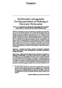
What about the categories denoted by the words “another” and “misfortune”? These are not direct, concrete sensory categories, but they still have examples in our direct sensorimotor experience: “That’s you” and “that’s another” (i.e., someone else). “That’s good fortune” and “that’s misfortune.” But it is more likely that higher-order, more abstract categories like these would be grounded in verbal definitions composed of words that each name already grounded categories, rather than being grounded in direct sensorimotor experience (Summers 1988; Aitchison 2012; Huang & Eslami 2013; Nesi 2014). Dictionary Grounding. This brings us to the question that is being addressed in this paper: A dictionary provides an (approximate) definition for every word in the language. Apart from a small, fixed set of words whose role is mainly syntactic (“function words,” e.g. articles, particles, conjunctions), all the rest of the words in the dictionary are the names of categories (“content words,” i.e. nouns, verbs, adjectives, adverbs). How many content words (i) – and which ones (ii) – need to be grounded already so that all the rest can be learned from definitions composed only out of those grounded words? We think the answer casts some light on how the meaning of words is represented – externally, in dictionaries, and internally, in our mental lexicon – as well as on the evolutionary origin and adaptive function of language for our species (Cangelosi & Parisi 2012; Blondin Massé et al. 2013). Synopsis of Findings. Before we describe in detail what we did, and how, here is a synopsis of what we found: When dictionaries are represented as graphs, with arrows from each defining word to each defined word, their graphs reveal a latent structure that had not previously been identified or reported, as far as we know. Dictionaries have a special subset of words (about 10%) that we have called their “Kernel” words. Figure 1 illustrates a dictionary and its latent structure using a tiny mini-dictionary graph (Picard, Lord, Blondin Massé, Marcotte, Lopes & Harnad 2013) derived from an online definition game that will be described later. A full-sized dictionary has the same latent structure as this mini-dictionary, but with a much higher proportion of the words (90%) lying outside the Kernel. Table 1 and Figure 2 show the proportions for a full-size dictionary. The dictionary’s Kernel is unique, and its words can define the remaining 90% of the dictionary (the “Rest”). The Kernel is hence a grounding set. But it is not the smallest grounding set. This smallest grounding subset of the Kernel – which we have called the “Minimal Grounding Set” (“MinSet”) – turns out to be much smaller than the Kernel (about 15% of the Kernel and 1% of the whole dictionary), but it is not unique: The Kernel contains a huge number of different MinSets. Each of these is of the same minimum size and each is able to define all the other words in the dictionary. The Kernel also turns out to have further latent structure: About 75% of the Kernel consists of a very big “strongly connected component” (SCC: a subset of words within which there is a definitional path to and from every pair of words but no incoming definitional links from experiences you can have are your own – there is no way to know for sure whether private experiences accompanied by the same public behavior are indeed identical experiences. These subtleties do not enter into the analyses we are doing in this paper. Word meaning is in any case not exact but approximate in all fields other than formal mathematics and logic. Even observable, empirical categories can only be defined or described provisionally and approximately: Like a picture or an object, an experience is always worth more than a thousand (or any number) of words (Harnad 1987).

outside the SCC). We call this the Kernel’s (and hence the entire dictionary’s) “Core.” The remaining 25% of the Kernel surrounding the Core consists of many tiny strongly connected subsets, which we call the Core’s “Satellites.” It turns out that each MinSet is part-Core and part Satellite. The words in these distinct latent structures also turn out to differ in their psycholinguistic properties: As we go deeper into the dictionary, from the 90% Rest to the 10% Kernel, to the Satellites (1-4%) surrounding the Kernel’s Core, to the Core itself (6-9%), the words turn out on average to be more frequently used (orally and in writing) and to have been learned at a younger age. This is reflected in a gradient within the Satellite layer: the shorter a Satellite word’s definitional distance (the number of definitional steps to reach it) from the Core, the more frequently it is used and the earlier it was learned. The average concreteness of the words within the Core and the 90% of words that are outside the Kernel (i.e., the Rest) is about the same. Within the Satellite layer in between them, however, Kernel words become more concrete the greater their definitional distance outward from the Core. There is also a (much weaker) definitional distance gradient from the Kernel outward into the 90% Rest of the dictionary for age and concreteness, but not for frequency. We will now describe how this latent structure was discovered. Control Vocabularies. Our investigation began with two small, special dictionaries – the Cambridge International Dictionary of English (47,147 words; Procter 1995; henceforth Cambridge) and the Longman Dictionary of Contemporary English (69,223 words; Procter 1978; henceforth Longman) (Table 1). These two dictionaries were created especially for people with limited English vocabularies, such as non-native speakers; all words are defined using only a “control” vocabulary of 2000 words that users are likely to know already. Our objective was to analyze each dictionary as a directed graph (digraph) in which there is a directional link from each defining word to each defined word. Each word in the dictionary should be reachable, either directly or indirectly, via definitions composed of the 2000-word control vocabulary. A direct analysis of the graphs of Longman and Cambridge, however, revealed that their underlying control-vocabulary principle was not faithfully followed: There turned out to be words in each dictionary that were not defined using only the 2000-word “control” vocabulary, and there were also words that were not defined at all. So we decided to use each dictionary’s digraph (a directed graph with arrows pointing from the words in each definition to the word they define) to work backward in order to see if we could generate a genuine control vocabulary out of which all the other words could be defined. (We first removed all undefined words.) Dictionaries as Graphs. Dictionaries can be represented as directed graphs 𝐷 = (𝑉, 𝐴) (digraphs). The vertices are words and the arcs connect defining words to defined words, i.e. there is an arc from word u to word v if u is a word in the definition of v. Moreover, in a complete dictionary, every word is defined by at least one word, so we assume that there is no word without an incoming arc. A path is a sequence (𝑣! , 𝑣! , … , 𝑣! ) of vertices such that (𝑣! , 𝑣!!! ) is an arc for 𝑖 = 1,2, … , 𝑘 − 1. A circuit is a path starting and ending at the same vertex. A graph is called acyclic if it does not contain any circuits. Grounding Sets. Let 𝑈 ⊆ 𝑉 be any subset of words and let u be some given word. We are interested in computing all words that can be learned through definitions composed only of

words in 𝑈. This can be stated recursively as follows: We say that u is definable from 𝑈 if all predecessors of u either belong to 𝑈 or are definable from 𝑈. The set of words that can be defined from 𝑈 is denoted by 𝐷𝑒𝑓 (𝑈). In particular, if 𝐷𝑒𝑓(𝑈) ∪ 𝑈 = 𝑉, then U is called a grounding set of 𝐷. Intuitively, a set 𝑈 is a grounding set if, provided we already know the meaning of each word in 𝑈, we can learn the meaning of all the remaining words just by looking up the definitions of the unknown words (in the right order). Grounding sets are equivalent to well-known sets in graph theory called feedback vertex sets (Festa, Pardalos & Resende (1999). These are sets of vertices 𝑈 that cover all circuits, i.e. for any circuit c, there is at least one word of c belonging to 𝑈. It is rather easy to see this. On the one hand, if there exists a circuit of unknown words, then there is no way to learn any of them by definition alone. On the other hand, if every circuit is covered, then the graph of unknown words is acyclic, which means that the meaning of at least one word can be learned – a word having no unknown predecessor (Blondin Massé et al 2008)). Clearly, every dictionary D has many grounding sets. For example, the set of all words in D is itself a grounding set. But how small can grounding sets be? In other words, what is the smallest number of words you need to know already in order to be able to learn the meaning of all the remaining words in D through definition alone? These are the Minimal Grounding Sets (MinSets) mentioned earlier (Fomin, Gaspers, Pyatkin & Razgon 2008). It is already known that finding a minimum feedback vertex set in a general digraph is NPhard (Karp, 1972), which implies that finding MinSets is also NP-hard. Hence, it is highly unlikely that one will ever find an algorithm that solves the general problem without taking an exponentially long time. However, because some real dictionary graphs are relatively small and also seem to be structured in a favorable way, our algorithms are able to compute their MinSets. Kernel. As a first step, we observed that in all dictionaries analyzed so far there exist many words that are never used in any definition. These words can be removed without changing the MinSets. This reduction can be done iteratively until no further word can be removed without leaving any word undefinable from the rest. The resulting subgraph is what we called the dictionary’s (grounding) Kernel. Each dictionary’s Kernel is unique, in the sense that every dictionary has one and only one Kernel. The Kernels of our two small dictionaries, Longman and Cambridge, turned out to amount to 8% and 7% of the dictionary as a whole, respectively. We have since extended the analysis to two larger dictionaries, Merriam-Webster (248,466 words; Webster 2006; henceforth Webster) and WordNet (132,477 words; Fellbaum 2010) whose Kernels are both 12% of the dictionary as a whole (Table 1). Core and Satellites. Next, since we are dealing with directed graphs, we can subdivide the words according to their strongly connected components. Two words u and v are strongly connected if there exists a path from u to v as well as a path from v to u. Strongly Connected Components (SCCs) are hence maximal sets of words with a definitional path to and from any pair of their words. There is a well-known algorithm in graph theory that computes all the SCCs very efficiently (Tarjan 1972). Sources are SCCs in which no word’s definition depends on a word outside the SCC (no incoming arcs). The Kernel of each of the four dictionary graphs turns out to contain an SCC much larger than all the others. One would intuitively expect the Kernel’s Core (as the union of Sources) to be that largest SCC.

And so it is in two of the four dictionaries we analyzed. But because of the algorithm we used in preprocessing our dictionaries, in the other two dictionaries the Core consists of the largest SCC plus a few extra (small) SCCs. We think those small extra SCCs are just an artifact of the preprocessing. In any case, for each of the four dictionaries, the Core amounts to 65%-90% of the Kernel or about 6.5%-9.0% of the dictionary as a whole. The SCCs that are inside the Kernel but outside the Core are called Satellites; collectively they make up the remaining 10%-35% of the Kernel or about 1.0%-3.5% of the whole dictionary. Satellites. Definitional Distance from the Kernel: the K-Hierarchy. Another potentially informative graph-theoretic property is the “definitional distance” of any given word from the Kernel or from the Core in terms of the number of arcs separating them. We define these two distance hierarchies as follows. First, for the Kernel hierarchy, suppose K is the Kernel of a dictionary graph D. Then, for any word u, we define its distance recursively as follows: 1. 𝑑𝑖𝑠𝑡(𝑢) = 0, if u is in K; 2. 𝑑𝑖𝑠𝑡(𝑢) = 1 + 𝑚𝑎𝑥{𝑑𝑖𝑠𝑡(𝑣) ∶ 𝑣 is a predecessor of 𝑢}, otherwise. In other words, to compute the distance between K, as origin, and any word u in the rest of D, we compute the distances of all words defining u and add one. This distance is well defined, because K is a grounding set of D and hence the procedure cannot cycle because every circuit is covered. The mapping that relates every word to its distance from the Kernel is called the K-hierarchy. Definitional Distance from the Core: the C-Hierarchy. The second metric is slightly more complicated but based on the same idea. Let D be the directed graph of a dictionary, and D’ be the graph obtained from D by merging each strongly connected component (SCC) into a single vertex. The resulting graph is acyclic. We can then compute the distance of any word from the Core (the vertex corresponding to the biggest of the merged strongly connected components of the Kernel) as follows: 1. 𝑑𝑖𝑠𝑡(𝑢) = 0, if u is in a source vertex of D’; 2. 𝑑𝑖𝑠𝑡(𝑢) = 1 + 𝑚𝑎𝑥{𝑑𝑖𝑠𝑡(𝑣) ∶ 𝑣 is a predecessor of 𝑤 for some 𝑤 in the same SCC as 𝑢}, otherwise. The words in the merged vertices of the Core have no predecessor and constitute the origin of the C-hierarchy. Like the K-hierarchy, the C-hierarchy is well defined because D’ is acyclic. MinSets. We have computed the Kernel K, Core C, and Set of satellites S as well as the Khierarchy and the C-hierarchy for four English dictionaries: two smaller ones – (1) Longman’s Dictionary of Contemporary English (Longman, 47,147 words), (2) Cambridge’s International Dictionary of English (Cambridge, 69,223 words) – and two larger ones - (3) Merriam-Webster (Webster, 248,466 words), (4) WordNet (132,477 words). Because of polysemy (multiple meanings)3, there can be more than one word with the same word-form 3 Once the problem of polysemy is solved for both defined and defining words, the analysis described in this paper can be applied to each unique word/meaning pair instead of just to the first meaning of each defined word.

(lexeme). As an approximation, for each stemmatized word-form we used only the first (and most frequent) meaning for each part of speech of that word-form (noun, verb, adjective, adverb). (This reduced the total number of words by 53% for Cambridge, 49% for Longman, 37% for Webster and 65% for WordNet.) The sizes of their respective Kernels turned out to be between 8% of the whole dictionary for the smaller dictionaries and 12% for the larger dictionaries. The Kernel itself varied from 10% Satellite and 90% Core for the two small dictionaries to 35% Satellite and 65% Core for the two large dictionaries (Table 1). As noted earlier, computing the MinSets is much more difficult than computing K, C, or S (in our current state of knowledge), because the problem is NP-hard. (Note that the most difficult part consists of computing MinSets for the Core, which can be further reduced by a few simple operations.) This problem can be modelled as an integer linear program whose constraints correspond to set-wise minimal circuits in the dictionary graph. The number of these constraints is huge but one can "add" constraints as they are needed. For the two "small" dictionaries (Longman and Cambridge), we were able to use CPLEX, a powerful optimizer, to compute a few MinSets (although not all of them, because there are a very large number of MinSets). For Webster and WordNet, the MinSets that we obtained after several days of computation were almost optimal.4 These analyses answered our first question about the size of the MinSet for these four dictionaries (373 and 452 words for the small dictionaries; 1396 and 1094 for the larger ones; about 1% for each dictionary). But because, unlike a dictionary’s unique Kernel, its MinSets are not unique, a dictionary has a vast number of MinSets, all within the Kernel, all the same minimal size, but each one different in terms of which combination of Core and Satellite words it is composed of. The natural question to ask now is whether the words contained in these latent components of the dictionary, identified via their graph-theoretic properties – the MinSets, Core, Satellites, Kernel and the rest of the dictionary – differ from one another in any systematic way that might give a clue as to the function (if any) of the different latent structures identified by our analysis.

4 This is yet another approximation in an analysis that necessitated many approximations: ignoring syntax and word order, using only the first meaning, and finding only something close to the MinSet for the biggest dictionaries. Despite all these approximations and potential sources of error, systematic and interpretable effects emerged from the data.

Figure 1. Illustration of a dictionary graph using data for a tiny (but complete) minidictionary (Picard et al 2013) generated by our dictionary game (see text for explanation). Arrows are from defining words to defined words. The entire mini-dictionary consists of just 32 words. Mini-dictionaries have all the latent structures of full-sized dictionaries. The smallest ellipse is the Core. The medium-sized ellipse is the Kernel. The part of the Kernel outside the Core is the Satellites. The part outside the Kernel is the Rest of the dictionary. There are many MinSets, all part-Core and part-Satellites (only one MinSet is shown here). In full-sized dictionaries the Rest is about 90% of the dictionary but in the game minidictionaries the Kernel is about 90% of the dictionary. The average Satellite-to-Core ratio in the Kernel for full-sized and mini-dictionaries is about the same (3/7) (see Table 1) but within MinSets this ratio is reversed (2/5 for full dictionaries and 5/2 for mini-dictionaries).

Cambridge Total word-meanings 47147 First word-meanings 25132 Rest 22891 (91%) Kernel 2241 (9%) Satellites 232 (1%) Core 2009 (8%) MinSets 373 (1%) Satellite-MinSets 59 (16%) Core-MinSets 314 (84%)

Longman 69223 31026 28700 (93%) 2326 (8%) 540 (2%) 1786 (6%) 452 (1%) 167 (37%) 285 (63%)

Webster

WordNet

248466 132477 91388 85195 80433 (88%) 75393 (88%) 10955 (12%) 9802 (12%) 2978 (3%) 3410 (4%) 7977 (9%) 6392 (8%) 1396 (2%) 1094 (1%) 596 (43%) 532 (49%) 800 (57%) 562 (51%)

Game dictionaries (average) 182 182 10.1 (7%) 171.7 (93%) 54.5 (29%) 117.2 (64%) 32.8 (18%) 20.6 (63%) 12.2 (37%)

Table 1. Number and percentage of word-meanings for each latent structure in each of the four dictionaries used (plus averages for game-generated dictionaries). Based on using only the first word-meaning for each stemmatized part of speech wherever there are multiple meanings (hence multiple words).

Figure 2. Overall pattern for average psycholinguistic differences (age of acquisition, concreteness, frequency) between words in latent structures revealed by the analysis of the dictionary digraph. Pattern is the same for all four dictionaries analyzed but image is not drawn to scale: for exact numbers and percentages see Table 1 and Figures 3 & 7). (MinSets are part Core and part Satellite. Core + Satellites = Kernel [~10%]. Outside the Kernel is the Rest [~90%]). Core words are more frequent (blue) and learned younger (orange) than the Rest of the dictionary. Within the Kernel’s Satellite layer, this difference increases gradually as definitional distance from the Core increases. Outside the Kernel, for age, the difference decreases gradually (but weakly) as definitional distance from the Kernel increases; frequency remains uniform. For concreteness (green), it is the Satellite layer that is more concrete than the Core. This difference increases gradually as definitional distance from the Core increases within the Satellite layer of the Kernel. Outside the Kernel, concreteness is at first equal to the Core and then increases gradually (but weakly) as definitional distance from the Kernel increases.

Psycholinguistic Correlates of Dictionary Latent Structure. A number of databases have been compiled that index various psycholinguistic properties of words (e.g., Wilson 1988). We used three of them: For word frequency, we used the SUBTLEXUS Corpus, which has been found to be more reliable than the widely used Kučera and Francis (1967) word frequency norms (Brysbaert & New, 2009). Raw frequencies range from 1 to over 2 million, with an average of 669 and with about 1% of the values over 5000. For our goal of determining the average frequency for different sets of words, instead of using raw frequency, we used the Lg10WF metric (log10(FREQcount+1)) to reduce the effect of extreme values. For concreteness, the Brysbaert, Warriner & Kuperman (2014) concreteness ratings for 40,000 common English word lemmas were used. For age of acquisition, we used the Kuperman et al. (2012) age-of-acquisition ratings for 30,000 English words. We tested whether the words in the latent components we identified in dictionary graphs differ systematically in frequency, concreteness or age of acquisition. Our overall pattern of findings (for all four dictionaries) is illustrated in Figure 2, which shows the latent structures of the dictionary: the 90% Rest and the 10% Kernel, and within it the Core surrounded by its Satellites. Shown also is one MinSet (just one of many); all MinSets are part Core and part Satellite. Based on the data for word frequency (blue), concreteness (green) and age of acquisition (orange) from the psycholinguistic databases, the words in the Core for all four dictionaries are more frequent and learned younger than the Satellite words, which are in turn more frequent and younger than the Rest of the dictionary. The Satellites are more concrete than the Core or the Rest. The average values for each of the psycholinguistic variables in each of the latent substructures are shown in Figure 3. The pattern is the same for all four dictionaries. Because the results are based on the entire population of each dictionary graph, no statistical tests were done. All differences would be highly significant because the number of words in each dictionary is so big. The effects themselves, however, are not very big; there are clearly many other factors underlying these variables apart from the dictionary latent structures.

Figure 3: Average age, concreteness and frequency of words in Core, Satellites, Kernel and Rest. The pattern is the same for all four dictionaries: The Core is youngest and most frequent, then the Satellites, then the Rest. The Satellites are more concrete than the Core and the Rest, which are about equal (but see the gradients in Figure 7.)

The effect size for each of the pairwise differences in Figure 3 is shown in Figure 4. Note that the biggest effect size tends to be for frequency. This may be because the psycholinguistic database coverage for frequency is close to 100% complete5 for all the words in all three latent structures, Core, Satellites and Rest, whereas the coverage for age and concreteness declines with frequency, especially for the two larger dictionaries (Figure 5). It is possible that the effect sizes for age and concreteness would have been larger, especially for the larger dictionaries, if the database coverage had been more complete. It is likely that the incompleteness of the data for age and concreteness is itself an indirect effect of word frequency: Age and concreteness data are lacking for the less frequent words6. All three variables – age, concreteness, and frequency – are intercorrelated (frequency/age: -0.5915; frequency/concreteness: 0.1583; age/concreteness: -0.3773). Decorrelating frequency from age and concreteness by recalculating effect sizes for only the residual variance left after removing the frequency variance reduces the effect sizes for age and concreteness (Figure 6). Age and concreteness data, which are much harder to gather than frequency data, are less available for less frequent words: “From a list of English words that one of the authors (M.B.) is currently compiling, we selected all of the base words (lemmas) that are used most frequently as nouns, verbs, or adjectives” (Kuperman et al 2012). “Because ratings are only useful for well known words, we used a cut-off score of 85% known. In practice, this meant that not more than 4 participants out of the average of 25 raters indicated they did not know the word well enough to rate it. This left us with a list of 37,058 words and 2,896 two-word expressions (i.e., a total of 39,954 stimuli)” (Brysbaert, Warriner & Kuperman 2014). This introduces a frequency bias into our analysis, because of missing age and concreteness data for less frequent words. This frequency bias could either be (1) helping to reveal valid effects, (2) spuriously inflating them or (3) spuriously reducing them (Figure 4); or (4) removing the frequency bias by decorrelating frequency could be masking valid effects (Figure 6). We think it is unlikely that word frequency causes concreteness or age effects. It is more likely that age of acquisition and concreteness are part of the cause of frequency effects. But the direction of causality cannot be resolved by the available data.

5 Words in our four dictionaries that had no values for SUBTELXus’ frequencies were assigned frequency value zero. The SUBTELXus frequency data were collected on a corpus used as the reference database; zero means the word never occurred in that corpus. 6 Brysbaert (personal communication) has noted that: “Dictionaries contain many words not known to most humans. This is particularly the case for Webster and WordNet, of which nearly half the words refer to chemical or biological science words (types of plants, animals, tissues)… For many of these words there are no values for concreteness or Age of Acquisition. However, certainly for concreteness the main reason is that the raters do not know the words. Only experts are able to rate these.”

Figure 4. Effect size and direction for the principal comparisons among Core, Satellites, Kernel and Rest for age, concreteness and frequency, for each of the four dictionaries. Note that the effect size for frequency tends to be the largest, then age, then concreteness.

Figure 5. Percentage of words in Core, Satellites and Rest for which psycholinguistic data were available for age and concreteness for each of the four dictionaries. (Frequency data not shown because they are at 100% for all dictionaries.) Note that the percentage of available data is lower for the two bigger dictionaries, and decreases from the Core to the Satellites to the Rest.

Figure 6. Effect size and direction for the principal comparisons among Core, Satellites, Kernel and Rest for age, concreteness and frequency, for each of the four dictionaries when correlation with frequency is removed. Age and concreteness effects are reduced considerably (cf. Figure 4), especially for the bigger dictionaries, in which the psycholinguistic database coverage for age and frequency was lower for the less frequent words (cf. Figure 7).

Definitional Distance Gradients. Alongside the main effects – the average differences in frequency, age and concreteness between the Core, Satellites and the Rest – our analysis also revealed two kinds of graded effects: The upper part of Figure 7 shows the gradient for the K-Hierarchy, which is the definitional distance from the Kernel to the words in the Rest of the dictionary (i.e. the number of definitional steps to reach a word starting from the Kernel). The first step in this gradient, from distance level 0 (the Kernel) to level 1 corresponds roughly to the main effects in Figure 3: For frequency there is a decrease from level 0 to 1 for all four dictionaries; then frequency is flat for all but Cambridge. For age there is an increase from level 0 to 1 (i.e., level 1 words are “older” – i.e., learned later – than the Kernel) for all four dictionaries, then descending slightly for all but WordNet. For concreteness there is a decrease (i.e., becoming more abstract) from 0 to 1, and then a gradual increase. Apart from the first step, from 0 to 1, the K-Hierarchy curves are hard to interpret because not only do the words at each succeeding distance level become fewer (Table 1) and less frequent, but the psycholinguistic database coverage for age (orange) and concreteness (green) is incomplete, especially for the two bigger dictionaries (Figure 8, left), many of whose rarer words are scientific, biological and technical terms. The lower part of Figure 7 shows the gradient for the C-Hierarchy, which is the definitional distance from the Core for words in the Satellite layer (i.e. the number of definitional steps to reach a Satellite word starting from the Core). Here the gradients are consistent for all four dictionaries and all three psycholinguistic variables: they are descending (less frequent) for frequency, rising (getting older) for age, and rising (getting more concrete) for concreteness. Here too the number of words diminishes at each distance level (Table 2), but for the two larger dictionaries there is a particularly marked decrease in database coverage for age (orange) and frequency (Figure 8, left). (This very visible negative correlation between definitional distance from the Core within the Satellite layer and psycholinguistic database coverage is probably due to the decline of word frequency with definitional distance from the Core within the Satellite layer (Figure 7, lower, blue). The red lines show the same effects when we analyze words that are present at the same level (intersection) in both large dictionaries (thick red line) and (separately) words that are present in both smaller dictionaries (thin red line).

Figure 7: Average age, concreteness and frequency at each level of the definitional distance hierarchy starting from the Kernel through the Rest of the dictionary (K-Hierarchy, above), and within the Kernel, starting from the Core through the Satellites (C-Hierarchy, below), for each of the four dictionaries. K-Hierarchy: for age there is a big increase from the Kernel to level 1 and then a slight decrease at higher levels; for concreteness a slight decrease from K to 1, then slight increase; for frequency a big decrease from K to 1, then mostly flat. C-Hierarchy: increases for age and concreteness and decreases for frequency. All effects are stronger in the smaller dictionaries. The thick red lines show that the pattern is the same when considering only those words that occur at the same level (intersection) in both bigger dictionaries. The thin red lines show the pattern for words that occur at the same level in both smaller dictionaries.

0 Cambridge 2241 Longman 2326 Webster 10955 WordNet 9802

1 15935 20555 59160 48186

2 9483 12231 38111 26186

0 2008 1786* 7976* 6391

1 127 248 1220 1270

2 51 159 640 683

Cambridge Longman Webster WordNet

3 4122 4966 19860 12642

3 26 (54) 66 425 443

4 5 1663 (2796) 730 1906 (3025) 611 9577 4396 (7615) 5379 2248 (4304)

4 20 34 (64) 245 308

5 4 14 153 252

K-Hierarchy 6 7 276 105 259 121 1904 666 989 609

C-Hierarchy 6 7 4 6 4 106 (287) 68 179 117 (275)

8 20 81 292 293

8 4 49 77

9 2 39 201 125

9 2 39 56

10 6 89 32

10 19 17

11 2 38 7

11 6 6

12 25 1

13 2 -

14 2 -

12 2

Table 2. Number of words at each level of the definitional distance hierarchy starting from the Kernel through the Rest of dictionary (K-Hierarchy, above), and, within the Kernel, starting from the Core through the Satellites (C-Hierarchy below), for each of the four dictionaries. Note that Figure 7 was truncated at the blue level past which frequencies became too low to be representative. Words past the truncation point were added to the blue value (total number of words for blue level shown in parentheses).

K-Hierarchy Percentage of Observations for Age 100%

93% 87% 84%85%86%

90%

C-Hierarchy Percentage of Observations for Age 100%

92%

90%

83%83% 82% 82%

80%

88% 86% 83%

83% 74% 69%

70%

60%

60% 56% 49% 44% 38% 34%

60% 46%48% 44%45%45%

50% 40%

48% 45% 41% 38% 35%

50% 40%

30%

30%

20%

20%

10%

10%

58% 45% 41% 30% 24% 21%

0%

0%

Cambridge

Longman

Webster

Cambridge

WordNet

K-Hierarchy Percentage of Observations for Concreteness 100%

94%

77%

80%

72%

69%

70%

93% 92% 94% 87%

98%

92% 92%92% 93%

90%

97% 94% 93% 92%

90%

100% 86%

Longman

98% 94%96% 93%

90%

83%

80%

99% 94% 95% 92% 86%

70% 60%

67% 63%

WordNet

70% 58%

54%

50%

60% 50%

50%

40%

40%

30%

30%

20%

20%

10%

10%

0%

93%

91% 80% 73% 66% 59% 57% 53%

80% 67% 67% 66%67%68%

Webster

C-Hierarchy Percentage of Observations for Concreteness 83% 71% 60% 53% 40% 35% 28%

0%

Cambridge

Longman

Webster

WordNet

Cambridge

Longman

Webster

WordNet



Figure 8. Percentage of words at each level of the definitional distance hierarchy starting from the Kernel through the Rest of dictionary (K-Hierarchy, left), and, only within the Kernel, starting from the Core through the Satellites (C-Hierarchy right), for which psycholinguistic data were available for age and concreteness for each of the four dictionaries. (Frequency data not shown because 100% for all dictionaries.) Note that the percentage of available data is lower for the two bigger dictionaries, and that within the Satellite layer it decreases with increasing definitional distance from the Core in the CHierarchy.

Core and Satellite Components of the MinSets. Because it takes so long to compute MinSets, even for the two small dictionaries, we do not have many of them yet; and for the two large dictionaries we so far only have one approximate MinSet each. Every MinSet is part-Core and part-Satellites. A natural question to ask is: What is the difference between the words in these two subcomponents of every MinSet? In the Kernel, the Core is more frequent, younger and less concrete than the Satellites. Comparing the words in the Core component of each MinSet with equal-sized random sets of Core words, and comparing the words in the Satellite component of each MinSet with equal-sized random sets of Satellite words also shows this ratio: For all four dictionaries, the Core component of the MinSet is more frequent, younger and less concrete than its random counterparts, and the Satellite component is less frequent, older and more concrete (Figure 9). (This effect was confirmed by t-tests (p