South-Eastern Europe Journal of Economics 2 (2011) 229-244

THE INTERRELATIONSHIP BETWEEN MERCHANDISE TRADE, ECONOMIC GROWTH AND FDI INFLOWS IN INDIA MOUSUMI BHATTACHARYA*, SHARAD NATH BHATTACHARYA Army Institute of Management, India

Abstract The purpose of the paper is to investigate whether the volume of merchandise trade and FDI inflows influences economic growth. The period of the study is 1996-97:Q1 to 2008-09:Q3. After investigating the stationarity of the variables, cointegration analysis has been conducted followed by VECM analysis and Granger Causality Test. The variables are I(1) processes. While unidirectional causality is observed from merchandise trade to economic growth, feedback causality has been observed between FDI inflows and economic growth. JEL Classification: F43 Keywords: FDI inflows, Multivariate Granger Causality Test,VECM, Co-integration Analysis, Economic growth.

*Corresponding Author: Mousumi Bhattacharya, Army Institute of Management, Judges Court Road, Command Hospital Complex, Kolkata-700027, West Bengal, India e-mail: [email protected]

230

M. BHATTACHARYA, S. N. BHATTACHARYA, South-Eastern Europe Journal of Economics 2 (2011) 229-244

Introduction Trade and foreign direct investment are often seen as important catalysts for economic growth in developing countries. Apart from acting as an important vehicle of technology transfer, FDI also stimulates domestic investment and facilitates improvements in human capital and institutions in the host countries. Trade also acts as an instrument of economic growth and facilitates efficient production of goods and services by shifting production to countries that have comparative advantage in producing them. The impact of FDI and trade on economic growth varies across countries depending upon certain factors like level of human capital, domestic investment, infrastructure, macroeconomic stability, and trade policies. India was basically a closed economy till 1985, characterized by infant industry protection, import licensing, a pegged exchange rate, foreign exchange controls and limited private sector participation. After the BOP crises in 1990-91, India embarked on a structural economic reform policy, called the New Economic Policy, envisioning gradual elimination of trade barriers, opening up of the real and financial sectors to foreign investments and encouragement to the private sector. After 1991 there was a marked change in the strategy followed by the government of India favouring export-oriented industrialization as opposed to import substituting industrialization, which it had followed in the past. Consequent upon the rationalization of tariffs and import duties as part of the NEP, there has been manifold increase in India’s trade with the rest of the world. For instance, total merchandise trade has increased from US$ 24.6bn in 1985 to US$ 41.8 bn in 1990, rising to US$ 93 bn in 2000 and US$ 402.7bn in 2007. The combined trade in goods and services confirms a similar trend of growth from US$ 30bn in 1985 to US$49.8bn in 1990, and further to US$126 bn and US$444.8 bn in 2000 and 2006 respectively, with the average growth during 2002-06 being 28.9% (Narayanan and Dash, 2010). India is gradually becoming more integrated with the world economy, with an expanding export sector. (Holmes et al. 2011). The purpose of this paper is to examine the causal relationship, if any, between the volume of India’s merchandise trade, Foreign Direct Investment (FDI) inflows and economic growth (GDP) in a Vector Auto Regressive (VAR) framework, during the post-liberalization period, and to ascertain the economic implications of such a causal relationship. Literature Review The positive relationship between economic growth and international trade has been well documented by Michaely (1977) and Balassa (1978). Feder (1983), Ram (1985), Salvatore (1991) and Hatcher (1991) in their studies have analysed the export-led growth hypothesis where they argued that exports are likely to alleviate foreign exchange constraints and thereby facilitate importation of better technologies

M. BHATTACHARYA, S. N. BHATTACHARYA, South-Eastern Europe Journal of Economics 2 (2011) 229-244

231

and production methods. In developing countries pursuing outward-oriented trade policies Balasubramanayam et al. (1996) found that FDI flows were associated with faster growth than in those developing countries that pursued inward-oriented trade policies. The causality between exports and economic growth for five countries of the Association of Southeast Asian Nations (ASEAN) was examined by Ahmad and Harnhirun (1996). Dutt and Ghosh (1996) studied causality between exports and economic growth for a relatively large sample of countries using the error correction model (ECM) for the countries in which they found cointegration. The VEC model was estimated, and tests for Granger causality were performed. Borensztein, Gregorio, and Lee (1998) examined the role of FDI in promoting economic growth using an endogenous growth model. They analyzed FDI flows from industrial countries to 69 developing countries during 1970-1989. Their results also show that FDI is an important vehicle of technology transfer, contributing more to economic growth than domestic investment. According to Goldberg and Klein (1998) direct investment may encourage export promotion, import substitution, or greater trade in intermediate inputs, especially between parent and affiliate producers. Along the same lines Blomstrom, Globerman and Kokko (2000) argue that the beneficial impact of FDI is only enhanced in an environment characterized by an open trade, investment regime and macroeconomic stability where FDI can play a key role in improving the capacity of the host country to respond to the opportunities offered by global economic integration. Empirical research by Chakraborty and Basu (2002) examined FDI and trade function as engines of growth, where they concluded that as trade and FDI liberalization policies began in India in the late 1980s and were widened in the 1990s, these policy liberalizations have increased growth in India significantly. Love and Chandra (2004) were of the same opinion and confirmed these results, going on to suggest that trade and economic growth exhibits a feedback relationship. Although there are some studies by Jung and Marshall (1985), Afxentiou and Serletis (1991), Bahmani-Oskooee et al. (1991), Love (1992) which have cast some doubt on the validity of the ELG hypothesis, the majority of the studies – for example Serletis (1992), Henrique and Sadorsky (1996), Bahmani- Oskooee and Alse (1993), Ghatak et al. (1995) and Nidugala (2001) - support the ELG hypothesis. The relationship between volume of merchandise trade and FDI inflows, and interpreting the importance of these activities towards economic growth, has always been considered an important topic for discussion, from the era of import liberalization policies to the era of openness and economic growth, although the empirical work on the relationship is relatively limited. Many of the studies conducted so far do not discuss the issue of causality between the three variables, and the existing literature on the Indian position in the subject matter proves to be inadequate. Although there are some studies by Dhawan and Biswal (1999), Asafu-Adjaye et al. (1999), Anwer and Sampath (2001), Nidugala (2001), Ghatak et al. (1997), Sharma and Panagiotidis

232

M. BHATTACHARYA, S. N. BHATTACHARYA, South-Eastern Europe Journal of Economics 2 (2011) 229-244

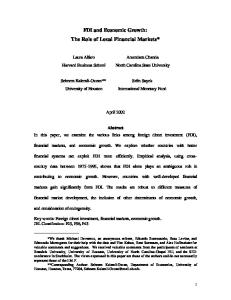
(2005) which have conducted causality analysis, most of them have taken total of exports, total of imports, whereas our study tries to specifically find out the effect of merchandise trade on economic growth along with the presence of FDI. Data The time period of the study is 1996-97: Q1 to 2008-09:Q3. Quarterly data relating to FDI inflows is collected from BOP statistics published by RBI and data of GDP (at 1999-00 market prices), while volume of merchandise trade (export + import) is taken from RBI Bulletins. Methodology In a multivariate Vector Autoregressive (VAR) framework the study has used the Granger-Causality Test to examine the causal links between economic growth, FDI inflows and volume of merchandise trade over the period 1996-97:Q1 to 2008-09:Q3. Figure 1. Logarithmic values of Foreign Direct Investment Inflows, Gross Domestic Product and Merchandise Trade

Tests for Stationarity Augmented Dickey Fuller (ADF) (1979), Phillips-Perron (PP) (1988) and Kwiatkowski, Phillips, Schmidt and Shin (KPSS) (1992) tests have been conducted to investigate the stationarity property of the series.

M. BHATTACHARYA, S. N. BHATTACHARYA, South-Eastern Europe Journal of Economics 2 (2011) 229-244

233

Tests for Cointegration To determine the long-run economic relationship between the variables a cointegration test has been conducted. In this study, the Error-correction Cointegration technique of Johansen (1988) and Johansen and Juselius (1990) has been applied to identify the cointegration relationship between the variables. This approach to the number of co-integrating vectors is applicable only if all the variables are I(1). According to Johansen (1988), a p-dimensional VAR model, involving up to k-lags can be specified as below. Z t = ∏1 Z t −1 + ∏ 2 Z t − 2 + .......... ∏ k Z t − k + ε t

(1)

where Zt is a ( p ×1) vector of p potential endogenous variables and each of the Π i is a ( p × p ) matrix of parameters and ε t is the white noise term. Equation (1) can be formulated into an Error Correction Model (ECM) form as below. k −1

DZ t = ∏ k Z t − k + ∑ θi DZ t −i + ε t

(2)

i =1

where D is the first difference operator, and Π and θ are p by p matrices of unknown parameters and k is the order of the VAR translated into a lag of k − 1 in the ECM, and ε t is the white noise term. Π is a vector which represents a matrix of long-run coefficients and it is of paramount interest. The long-run coefficients are defined as multiples of two ( p × r ) vectors, α and β ' , and hence Π = αβ ' , where α is a vector of the loading matrices and denotes the speed of adjustment from disequilibrium, while β ' is a matrix of long-run co-efficients so that the term β ' Z t −1 in equation (2) represents up to ( p − 1) cointegration relationships in the Cointegrating Model. Evidence of the existence of cointegration is the same as evidence of the rank ( r ) for the Π matrix. Johansen and Juselius (1990) showed that the rank ( r ) of Π matrix in equation (2) is equal to the number of cointegrating vectors in the system. If it has full rank i.e. r = p (in the present study if Π = 2 ) it is said that there are p cointegrating relationships and that all variables are I(0). If the rank r = 0 then it implies that the sequences are unit root processes and there is no cointegration and the appropriate model is a VAR in the first differences involving no long run element. If the rank is reduced [ 1 ≤ Rank Π ≤ ( p − 1) ], even if all the variables are individually I(1), the level based long run component would be stationary. The appropriate modelling methodology here is the Vector-Error Correction Model (VECM). Two Likelihood Ratio Tests were developed by Johansen and Juselius (1990). The first test is the Likelihood Ratio Test based on the maximal Eigen value, which evaluates the null hypothesis of ‘ r ’ cointegrating vector(s) against the alternative of ‘ r + 1 ’ cointegrating vectors. The other Likelihood Ratio Test is based on the Trace

234

M. BHATTACHARYA, S. N. BHATTACHARYA, South-Eastern Europe Journal of Economics 2 (2011) 229-244

test, which evaluates the null hypothesis of, at most, ‘ r ’ cointegrating vector(s) against the alternative hypothesis of more than ‘ r ’ cointegrating vectors. If the two variables are I(1), but cointegrated, the Granger Causality Test will be applied in the framework of ECM in which long-run components of the variables obey equilibrium constraints while the short-run components have a flexible dynamic specification. Test for Granger Causality with VECM The Granger Causality Test has been conducted in order to examine the causal linkages between the variables. The direction of the impact of each of the variables is also determined from the analysis. In order to capture the impact of variables observed in the past time period in explaining the future performance, the optimal lag length p (which is 4 in the present study) is chosen (see Table 1) and the criteria used in selecting the VAR model and optimal lag length require the combination of information criterion (minimum of AIC and SIC). Table 1. VAR Lag Order Selection (D.LnGDP, D.LnFDI, D.MERTRADE)



* indicates lag order selected by the criterion. D. represents the first difference of logarithmic values of the concerned variables.

Engle and Granger (1987) showed that there is possibility of a causal relationship in at least one direction when two series are integrated of order one [i.e. I (1)] and are cointegrated. The direction of a causal relationship can be detected in the VECM. In the presence of cointegration, there always exists a corresponding error-correction representation, captured by the error-correction term (ECT). The ECT captures the long-run adjustment of cointegration variables. The incorporation of ECT in the VECM allows detecting both short- and long-run causal relationships between the variables

M. BHATTACHARYA, S. N. BHATTACHARYA, South-Eastern Europe Journal of Economics 2 (2011) 229-244

235

Findings Stationarity Test Table 2 reports the results of the ADF, PP and KPSS Tests of unit root by lag length chosen based on minimum values of SIC. The tests are performed on both the level and first differences of the lagged variables. The variables LnFDI, LnGDP and LnMERTRADE are I(1) processes according to ADF, PP and KPSS tests. Table 2. Test of Unit Root Test Hypothesis (1996-97:Q1 –2008-09:Q3) without trend

(a) The critical values are those of MacKinnon (1991). 1% ADF-Critical Value = -3.571310 in case of LnFDI and its first difference. 1% ADF-Critical Value = -3.581152; 5% ADF-Critical Value = -2.926622; 10% ADF- Critical Value = -2.601424 in case of LnGDP (logarithmic value of GDP) and its first difference. 1% ADF-Critical Value = -3.577723 in case of LnMERTRADE and its first difference. 1% PP-Critical Value = -3.568308; 5% PP-Critical Value = -2.921175; 10% PP-Critical Value = -2.598551 in case of LnFDI, LnGDP, LnMERTRADE. 1% PP-Critical Value = -3.571310; 5% PP-Critical Value = -2.922449; 10% PP-Critical Value = -2.599224 in case of first difference of LnFDI, LnGDP, LnMERTRADE. 1% KPSS-Critical Value = 0.739; 5% KPSS-Critical Value = 0.463; 10% KPSS-Critical Value = 0.347 in case of LnFDI, LnGDP, LnMERTRADE and its first difference. (b)***, ** and * represent the rejection of null hypothesis at the 1%, 5% and 10% level of significance respectively.

236

M. BHATTACHARYA, S. N. BHATTACHARYA, South-Eastern Europe Journal of Economics 2 (2011) 229-244

Cointegration Test Table 3 presents the results of the Johansen Cointegration Test. Going by the results of the ADF, PP and KPSS tests it has been observed that the variables have the same order of integration, i.e., I(1) and the Johansen Cointegration Test has been employed to find out the cointegration rank and the number of cointegrating vectors. The null hypothesis of r = 0 (i.e., there is no cointegration) is rejected against the alternative hypothesis of r = 1 at the 5% level of significance in case of the Max-Eigen value statistic. Similarly, going by the result of the Trace statistic, the null hypothesis of r = 0 is rejected against the alternative hypothesis of r ≥ 1 . Table 3. Johansen -Juselius Co integration Test Results [no deterministic trend (restricted constant)]



(a) is the number of cointegrating vectors. (b)** denotes rejection of the null hypothesis at the 5% level of significance (c)The critical values (i.e., CVs) are taken from Mackinnon-Haug-Michelis (1999).

To test whether each co-efficient in a cointegrating equation was statistically zero and can be excluded from the set of co-integrating relations, restrictions may be imposed on the cointegrating vector. Restrictions can be placed on the co-efficients β ( r , k ) of the r th co-integrating relation:

β (r ,1) LnFDI + β (r , 2) LnGDP + β (r ,3) LnMERTRADE The statistical significance of these restrictions is provided by the Chi-square statistic, with degrees of freedom equal to the number of restrictions. In Table (4a), the null hypothesis that co-efficient of LnFDI is not significantly different from zero can be rejected because of the low probability value of 0.000700. In Table 4(b), the null hypothesis that co-efficient of LnGDP is not significantly different from zero can be rejected because of the low probability value of 0.022422. In Table 4(c), the null hypothesis that co-efficient of LnMERTRADE is not significantly different from zero can also be rejected because of the low probability value of 0.000243.

M. BHATTACHARYA, S. N. BHATTACHARYA, South-Eastern Europe Journal of Economics 2 (2011) 229-244

237

Table 4a. VEC Co-efficient Restrictions

Table 4b. VEC Co-efficient Restrictions

Table 4c. VEC Co-efficient Restrictions

From the above observations, it can be said that the restriction imposed on LnFDI, LnGDP, LnMERTRADE can be rejected by using the LR test statistic. The test result suggests that the linear combinations of all variables is co-integrated, and are equally influential.

238

M. BHATTACHARYA, S. N. BHATTACHARYA, South-Eastern Europe Journal of Economics 2 (2011) 229-244

Analysis of VECM Long-run relationship is observed among the variables under study as revealed by Johansen’s λmax and λtrace statistics (Table 3), thus justifying the use of ECM for showing short-run dynamics. The Granger Representation Theorem (Engle and Granger, 1987) states that if a set of variables is cointegrated, then there exists a valid error correction representation of the data. In Table 5, the cointegrating equations are given along with the equation for changes in FDI (first column), changes in GDP (second column), changes in merchandise trade (third column). The co-efficients of ECT contain information about whether the past values affect the current values of the variable under study. A significant co-efficient implies that past equilibrium errors has a role in determining the current outcomes. The information obtained from the ECM is related to the speed of adjustment of the system towards long-run equilibrium. The short-run dynamics are captured through the individual co-efficients of the difference terms. The adjustment co-efficients on ECTt − 2 are negative and statistically significant at the 1% level of significance indicating that, when deviating from the long-term equilibrium, error correction term has an opposite adjustment effect and the deviation degree is reduced. The significant error term also supports the existence of long-term relationship between the independent variables and economic growth in the long term. The lagged co-efficients of DFDI t −1 are positive and statistically significant at 1% level of significance indicating higher FDI inflows have a positive effect on economic growth in the short term. The lagged co-efficients of DMERTRADEt −1 , DMERTRADEt −3 , DMERTRADEt − 4 are negative and statistically significant at 1% level of significance and DMERTRADEt − 2 is negative at 5% level of significance implying that higher merchandise trade has a negative effect on economic growth in the short term. The lagged co-efficients of DGDPt −1 , DGDPt −3 are positive and statistically significant at 5% level of significance and DGDPt − 4 is positive and statistically significant at 10% level of significance implying that higher GDP has a positive impact on merchandise trade in the short term. Table 5. Vector Error Correction Estimates (Included observations: 46 after adjustments)

M. BHATTACHARYA, S. N. BHATTACHARYA, South-Eastern Europe Journal of Economics 2 (2011) 229-244

239

240

M. BHATTACHARYA, S. N. BHATTACHARYA, South-Eastern Europe Journal of Economics 2 (2011) 229-244

(a) ***, ** and * denotes statistical significance at 1%, 5% and 10% level of significance respectively. (b) Standard errors in ( ) & t-statistics in [ ]

Causality Test with VECM In Table 6 the causality Test with VECM is presented. The null hypothesis that LnGDP, LnMERTRADE do not Granger cause LnFDI is tested using changes in FDI Inflows (DLnFDI), changes in merchandise trade (DLnMERTRADE) and changes in gross domestic product (DLnGDP) when all of them are stationary in their first difference form in standard Granger causality regression. The null hypothesis is accepted or rejected based on “chi-squared test based on Wald criterion” to determine the joint significance of the restrictions under the null hypothesis. The lag length is justified by a minimum Final Prediction error (FPE), Schwarz Information Criterion (SIC) and likelihood ratio test statistics. The test result suggests lag order of 4 as optimal lag. The p value (0.0958) (Table 6) indicates that the coefficients of LnGDP are not jointly zero in the equation for LnFDI. In this case the null hypothesis that GDP does not Granger cause FDI Inflows can be rejected and an unidirectional causality is observed from gross domestic product to FDI Inflows.

M. BHATTACHARYA, S. N. BHATTACHARYA, South-Eastern Europe Journal of Economics 2 (2011) 229-244

241

Table 6. VEC Granger Causality/Block Exogeneity Wald Tests (Sample: 1 to 51)

The null hypothesis that LnFDI, LnMERTRADE do not Granger cause LnGDP is tested using changes in FDI Inflows (DLnFDI), changes in merchandise trade (DLnMERTRADE) and changes in gross domestic product ((DLnGDP) when all of them are stationary in their first difference form in Standard Granger causality regression. The p value (0.0052) (Table 6) indicates that the coefficients of LnFDI are not jointly zero in the equation for LnGDP. In this case the null hypothesis that LnFDI does not Granger cause GDP can be rejected and an unidirectional causality is observed from FDI Inflows to gross domestic product. The p value (0.0001) (Table 6) indicates that the coefficients of LnMERTRADE are not jointly zero in the equation for LnGDP. In this case the null hypothesis that LnMERTRADE does not Granger cause GDP can be rejected and an unidirectional causality is observed from merchandise trade to gross domestic product. It is observed that there is existence of a long-run relationship between GDP and FDI inflows i.e. presence of bi-directional causality between the two variables. A unidirectional causality is also observed from merchandise trade to economic growth.

242

M. BHATTACHARYA, S. N. BHATTACHARYA, South-Eastern Europe Journal of Economics 2 (2011) 229-244

Conclusion Feedback causality is observed between foreign direct investment inflow and economic growth. The government is planning for more liberalization measures across a broad range of sectors (agriculture, industry and services), which will further accelerate the inflow of FDI. The results reveal that FDI is growth-enhancing in the same way as domestic investment and a statistically significant effect exists in the sense that a higher ratio of FDI in the gross capital formation has positive effects on the level of GDP and hence on growth. It can be concluded that India’s capacity to progress will depend to a certain extent on the country’s performance in attracting foreign capital. India’s fiscal policy reforms along with a strong political mandate is expected to improve sentiment for the country’s economic outlook which in turn should improve its overall share in capital flows marked for emerging markets. This is indicated by the fact that despite the global slowdown, India has managed to display resilience and attract good investments. In the Indian context, FDI is encouraging the adoption of new technology in the production process through capital spillovers. Moreover it is also stimulating knowledge transfers both in terms of labour training and skill acquisition and by introducing alternative management practices and better organizational arrangements. The fact that dynamism of merchandise trade will accelerate economic growth in the country is revealed by the results obtained from the study i.e. unidirectional causality is observed from merchandise trade to economic growth. It is seen that India promoted exporting as a way to enhance economic growth, alongside a struggle to reform domestically, remove or simplify import restrictions, ensure political stability, encourage investment and alleviate poverty, which should also improve output and lead, in time, to further exporting. It is also observed that exporting, investment, trade shocks and output are intricately linked with each other and that export promotion is only one arm of economic development - investment, political and macroeconomic stability, internal reforms and other domestic policies are equally crucial. The government of India and RBI has taken various trade policy measures to mitigate the adverse impact of the global recession on the Indian economy and on checking inflation. Among the various measures taken include three stimulus packages announced in 2008-09, the measures by RBI and the Government in the Union Budget 2009-10 and the Foreign Trade Policy (2009-14) to help the export sector in general and employment intensive sectors affected by the world recession in particular. While short term relief and stimulus measures have worked in the Indian case, however some fundamental policy changes are needed and India needs to take bold steps towards reforms as it did in 1991 on the balance of payment crises and thus force the wavering leaders of liberalization and globalization not to backtrack. The results suggest that the ELG hypothesis is followed in case of India and the reform measures seem to have worked.

M. BHATTACHARYA, S. N. BHATTACHARYA, South-Eastern Europe Journal of Economics 2 (2011) 229-244

References

243

Afxentiou, P. C. and Serletis. A., 1991, “Exports and GNP Causality in the Industrial Countries: 1950-1985”, Kyklos, 44(2), 167-179. Ahmad, J. and Harnhirun, S., 1996, “Cointegration and Causality between Exports and Economic growth: Evidence from the ASEAN countries”, Canadian Journal of Economics, 29, 413 – 416 Anwer, M. S. and Sampath, R. K., 2001, “Exports and Economic Growth”, Indian Economic Journal, 47(3), 79-88. Asafu-Adjaye, J. and Chakraborty, D., 1999, “Export-led Growth and Import Compression: Further Time Series Evidence From LDCs”, Australian Economic Papers, 38, 164-75. Bahmani-Oskoee, M., Mohtadi, H. and Shabsigh, G., 1991, “Exports, Growth and Causality in LDCs: A Re- examination”, Journal of Development Economics, 36, 405-415. Bahmani-Oskoee, M. and Alse, J., 1993, “Export Growth and Economic Growth: An Application of Cointegration and Error-Correction Modelling”, Journal of Development Areas, 27, 535-542. Balassa, B., 1978, “Exports and Economic Growth: Further evidence”, Journal of Development Economics, 5(2), 181-189. Balasubramanyam, V. N., Salisu, M. A. and Sapsford, D., 1996, “Foreign Direct Investment and Growth in EP and IS Countries”, Economic Journal, 106(434), 92-105. Blomstrom, M., Globerman, S. and Kokko, A., 2000, “The Determinants of Host Country Spillovers from Foreign Direct Investment”, CEPR, Discussion Paper No.2350. Borensztein, E. J., Gregorio, D. and Lee, J. W., 1998, “How does foreign direct investment affect economic growth?”, Journal of International Economics, 45(1), 115-135. Chakraborty, C. and Basu, P., 2002, “Foreign Direct Investment and Growth in India: A Cointegration Approach”, Applied Economics, 34(9), 1061-1073. Dhawan, U. and Biswal. B., 1999, “Re-examining export led growth hypothesis: a multivariate cointegration analysis for India”, Applied Economics, 31,525-30. Dickey, D.A. and Fuller, W.A., 1979, “Distribution of the estimations for autoregressive time series with a unit root”, Journal of American Statistical Association, 74, 423-31. Dutt, S.D. and Ghosh, D., 1996, “The Export Growth Economic Growth Nexus: A Causality Analysis”, The Journal of Developing Areas, 30, 167-182. Engle, R.F. and Granger, C.W.J., 1987, “Cointegration and Error-Correction: Representation, Estimation, and Testing”, Econometrica, 55, 251-276. Feder, G. 1983, “On Exports and Economic Growth”, Journal of Development Economics, 12, 59-73. Ghatak, S and Price. S. W., 1995, “Export Composition and Economic Growth: Cointegration and Causality Evidence for India”, Weltwirtschaftliches Archiv, 133(3), 538-553. Ghatak, S, C. Milner and Utkulu, U., 1997, “Exports, export composition and growth: cointegration and causality evidence for Malaysia”, Applied Economics, 29, 213-23. Goldberg, S. and Klein, W., 1998, “Foreign Direct Investment and Real Exchange Rate Linkages in Developing Countries” in Reuven Glick (Ed.) Managing Capital Flows and Exchange Rates: Lessons from the Pacific Basin, Cambridge University Press. Henriques, I. and Sadorsky, P., 1996, “Export-led growth or growth-driven exports? The Canadian case”, Canadian Journal of Economics, 29(3), 540-555. Holmes, M.J., Panagiotidis T. and Sharma, A., 2011, The sustainability of India’s current account, Applied Economics, 43 (2), 219-229. Johansen, S., 1988,“Statistical Analysis of Co-integrating Vectors”, Journal of Economic Dynamics and Control, 12, 231-254. Johansen, S. and Juselius, K., 1990, “Maximum Likelihood Estimation and Inference on Cointegration with Application to the Demand for Money”, Oxford Bulletin of Economics and Statistics, 52, 169-210.

244

M. BHATTACHARYA, S. N. BHATTACHARYA, South-Eastern Europe Journal of Economics 2 (2011) 229-244

Jung, W. S. and Marshall, P. J., 1985, “Exports, Growth and Causality in Developing Countries”, Journal of Development Economics, 18, 1-12. Kwiatkowski, D., Phillips, P.C.B, Schmidt, P. and Shin, Y., 1992, “Testing the Null Hypothesis of Stationarity against the Alternative of a Unit Root”, Journal of Econometrics, 54, 159-178. Love, J., 1992, “Export Instability and the Domestic Economy: Questions of Causality”, Journal of Development Studies, 28(4), 735-42. Love, J. and Chandra, R., 2004, “Testing Export-Led Growth in India, Pakistan, and Sri Lanka Using a Multivariate Framework”, The Manchester School, 72(4), 483-496. MacKinnon, J.G., 1991,“Critical Values for Co-integration Tests” in Engle R.F. and Granger C.W.J. (eds.), Long Run Economic Relationships: Readings in Co-integration, Oxford: Oxford University Press, 267-276. MacKinnon, J.G and Haug, A. A, and Michelis, L., 1999, “Numerical Distribution Functions of Likelihood Ratio Tests for Cointegration,” Journal of Applied Econometrics, 14(5), 563-77. Michaely, M., 1977, “Exports and Growth: An Empirical Investigation”, Journal of Development Economics, 4(1), 49-53. Narayan, K. and Dash, P., 2010, “Trade Dynamics and Foreign Exchange Reserves Management in India: An Empirical Study,” Journal of Applied Finance, 16(4), 5-28. Nidugala, G K., 2001, “Exports and Economic Growth in India: An Empirical Investigation”, Indian Economic Journal, 47(3), 67-78, Phillips, P.C.B and Perron, P., 1988, “Testing for a Unit Root in Time Series Regression”, Biometrika, 75, 335–346. Ram, R., 1985, “Exports and Economic Growth: Some Additional Evidence”, Economic development and Cultural change, 33(2), 415-425. Salvatore, D. and Hatcher, T., 1991, “Inward and Outward oriented trade strategies”, Journal of Development Studies, 27, 7-25. Serletis, A., 1992, “Export growth and Canadian economic development”, Journal of Development Economics, 38,133-45. Sharma A. and Panagiotidis T., 2005, “An Analysis of Exports and Growth in India: Cointegration and Causality Evidence (1971-2001)”, Review of Development Economics, 9(2), 232-248.