Södertörns högskola | Institutionen för Samhällsvetenskaper Magisteruppsats 30 hp |Nationalekonomi | Värterminen 2011

The effects of exchange rate volatility on export – Empirical study between Sweden and Germany

Av: Anh Mai Thi Van Handledare: Xiang Lin

Abstract The relationship between exchange rate volatility and trade flow has been examined in a number of previous researches. The paper mainly focuses on investigating the impact of exchange rate volatility on export values from Sweden to Germany during 2000:01 and 2011:06. The Auto Regressive Distributed Lag (ARDL) model is employed to obtain the estimates of the long run equilibrium and the short run dynamics, simultaneously. The results indicate that the exchange rate volatility has significant short run effects on export value in majority of estimated industries while its meaningful long run impacts do not appear in any cases. However, applying the “bounds test” approach, the co-integration is also found in more than half cases due to long run impacts of other factors such as foreign income on export earnings. Keywords: exchange rate, volatility, export, short run effects, long run effects, ARDL, Swedish krona, euro.

2

Acknowledgements Exchange rate, trade and their relationship are familiar topics in economics so searching and determining a different approach is the most difficult step in this paper. This task took me much time to handle during the thesis working period. Besides, constructing the ARDL model then running the diagnostic tests offered me a wonderful time to read and gain more new knowledge from previous studies. I would like to express my sincere thank to Professor Xiang Lin (Doctoral Degree in Economics, Department of Economics, Södertörns University) for his encouragement and instruction during my thesis working period. My special thanks to my family, my friends for their inspiration and motivations. They always support; advise me to overcome the difficulties during the completion of this paper.

Anh Mai Thi Van Stockholm, January 13, 2012

3

Contents

Abstract..................................................................................................................................... 2 Acknowledgements ................................................................................................................... 3 Contents .................................................................................................................................... 4 1. Introduction...................................................................................................................... 6 2. Literature Review ............................................................................................................. 9 2.1. Trade theories ............................................................................................................... 9 2.2. Exchange rate regime.................................................................................................. 10 2.3. Impact of exchange rate on trade flow......................................................................... 12 3. Early studies .................................................................................................................... 17 3.1. Negative effects .......................................................................................................... 17 3.2. Positive effects ........................................................................................................... 18 3.3. Ambiguous effects ...................................................................................................... 19 4. Actual export, exchange rate and its volatility development ......................................... 21 4.1. Bilateral export flows.................................................................................................. 21 4.2. Bilateral exchange rate................................................................................................ 23 4.3. Exchange rate volatility .............................................................................................. 26 5. Econometric Methodology .............................................................................................. 28 6. Econometric Modeling .................................................................................................... 31 7. Empirical results ............................................................................................................. 33 7.1. Stationary Test ............................................................................................................ 33 7.2. Optimal lags ............................................................................................................... 34 7.3. Short run analysis ....................................................................................................... 35 7.4. Long run analysis ....................................................................................................... 36 7.5. Diagnostic Tests ......................................................................................................... 39 8. Conclusion ....................................................................................................................... 41 Reference ................................................................................................................................ 43 Appendix ................................................................................................................................. 48 A. Data source ................................................................................................................... 48 4

B. Table ............................................................................................................................. 49 Table 1: Dickey-Fuller (DF) Test.............................................................................................. 33 Table 2: Optimal lags ............................................................................................................... 34 Table 3: Short run coefficient estimates of Sweden export model ............................................. 49 Table 4: Long run coefficient estimates of Sweden export model.............................................. 51 Table 5: Diagnostic tests ........................................................................................................... 52 Figure 1: The J-curve................................................................................................................ 14 Figure 2: Profits of the firm under price certainty and uncertainty............................................. 18 Figure 3: Total export values from Sweden to Germany (in billion SEK) .................................. 21 Figure 4: Nominal and real exchange rate development ............................................................ 25 Figure 5: Evolution of the exchange rate volatility defined as the first method: 12-month rolling window of the standard deviation in the past monthly real exchange rate ....................... 27

5

1. Introduction Since

March

1973

when

the

Bretton

Woods,

an

international

system of monetary management, collapsed, the major currencies have been floating with respect to each other instead of fixed ones based on the US dollar. Besides, export is considered as one of fundamental factors which contribute to the economic growth. To explicitly understand about the effects of exchange rate and its volatility on trade flow specifically in export, many previous papers, both theoretical and empirical ones, have investigated these relationships and provided various results. The exchange rate uncertainty may either hurt to financial market participants or create more opportunities for them. According to Engel & Нakkiо (1993), the wide spread of exchange rate variability have important adverse consequenses. For the investors, depending on their risk aversion, alteration on investment decision in short term will affect the cash flow of the economic market in the long term. For the trading firms, more volatile exchange value of foreign sales, more reluctant for firms to engage in the international trade. Moreover, Grauwe (1988) summazises that there has been a reduction in the growth rate of international trade more than 50% since the floating regime is applied. However, following Atish R. Ghosh et al. (1996), trade growth, measured as the sum of export growth and import growth, is almost 3% points higher under floating rates. The question of exchange rate volatility and trade has generated

much

interesting discussion recently because of many previous ambiguous ideas. The exchange rate affects trading flow within a given country differently due to dissimilar in economic factors. Sweden, a small size economy in Europe, is included in limited previous researches. The majotity of those papers concentrate on using either import or export data of Sweden with the rest of the world (e.g. Kenen & Rodrik, 1986; J. G. Thursby & Thursby, 1987; Qian & Varangis, 1994). Consequently, the implicit assumptions may be carried due to the problems of aggregation bias. Germany is still the largest and most potential 6

Sweden’s trading partner in the world until now. The bilateral export data from Sweden to Germany is not expected to suffer from aggregation bias which occurs when model is estimated on aggregate data. Moreover, by adopting data on different individual product group levels, the group bias phenomenon is probably avoided. In this paper, the Auto Regressive Distributed Lag (ARDL) bound testing procedure is adopted because of its three major advantages. The main advantage of this approach is to deal with nonsense relationship. In fact, there is a risk of a pure spurious correlation when nonstationary independent series are included in the regression. Thus, ARDL model is applied to yield consistent estimates of the long run coefficients that are asymptotically normal irrespective of whether the underlying time-series are I(1) or I(0) (Pesaran, 1999). Another advantage of ARDL approach is to obtain both short run and long run effects in a single equation. Moreover, this technique is suitable for small sample size (Pesaran, 1999). The aim of this study is therefore to examine the effects of exchange rate and its volatility on export values from Sweden to Germany by using monthly bilateral data from Jan 2000 to Jun 2011. Furthermore, the paper aims to determine the level of exchange rate or its volatility affecting export value in short run or long run. This study will investigate these relationships in total export value and ten distinct groups of commodities with biggest values: 07 - Metal ores; 17 - Paper and paper products; 19 - Coke and refined petroleum products; 20 - Chemicals and chemical products; 21 - Basic pharmaceutical products and pharmaceutical preparations; 24 - Basic metals; 26 - Computer, electronic and optical products; 27 - Electrical equipment; 28 - Machinery and equipment; 29 - Motor vehicles, trailers and semi-trailers. (Source: SCB). Beside the export value, exchange rate and its volatility, the industrial production index (IPI) of Germany which represented for Germany income is included in the main regressions.

7

The discussion of this topic is crucial and necessary to help the single firms or government policymakers react to the exchange rate fluctuation. Following evidences obtained in the paper, a number of new insights in the choice and implementation of exchange rate and trading policy are offered. In addition, this paper is one more evidence to confirm the whether there are long run or short run or both impacts of exchange rate and its variability on the export values. The results may also guide the trading firms to focusing on factors that may be more likely than others to affect export revenues. This paper shall focus merely on making a survey of total value and 10 main groups of commodities with highest values of export from Sweden to Germany in more than 10 years. Thus, the rest of industries in Sweden were not studied in this paper. Besides, Sweden import from Germany was not examined as well. As such, the results of Sweden trade balance after krona appreciation or depreciation against euro were not provided. The structure of this paper is organized as follows. After introduction, the second and the third section present the theories and studies of exchange rate, its volatility, trading and their relationships. The fourth part introduces all of data using for econometric modeling, including both of data construction and analysis. Section 5 discusses Econometric Methodology, Econometric Modeling is revealed in section 6. Section 7 describes some of the insight from the empirical results on their relationship. Finally, the concluding section gives the general overview of this paper and detailed empirical results are provided in the appendix

8

2. Literature Review 2.1. Trade theories The primary aim in this section is to present the related international trade theories and their developments. Pioneered by Adam Smith in 1776, the classical economic trade theory describes that a country has absolute advantage in ability to produce more goods or service than other countries, using the same amount of resources. Later, in the early 19th century, David Ricardo develops the theory of comparative advantage, which is the starting point of the international trade theories. The country has the comparative advantage in producing a product in terms of other products if it has lower opportunity cost than other countries. Moreover, if each country exports the goods in which it has a comparative advantage, both countries can gain benefits from trading between their borders (Krugman & Obstfeld, 2008, p. 29). However, Ricardian model is approached merely by comparing the differences in the productivity of labor. Developing from the trade theory of David Ricardo, Eli Heckscher and Bertil Ohlin, two Swedish economists, try to explain why certain countries have comparative advantages for certain goods with assumption of no differences in technological knowledge in two countries. Following Heckscher- Ohlin (H-O) model, a country will export products that use national abundant and cheap factor(s) and import products that use the countries' scarce factor(s) (Blaug, 1992, p. 190). H-O theory also refers to the factor-proportions theory because it emphasizes the proportions in different production’s factors which are used in producing goods in different countries. Since H-O theory is one of the most influent ideas in the international economics, there have been some empirical results against it. Trade often does not run in the direction that the H-O theory predicts (see further in Krugman & Obstfeld, 2008, p. 75).

9

Regarding Krugman & Obstfeld, the standard trade model was built based on 4 key relationships as result of many diverse effects of trade changes on various countries. “(l) the relationship between the production possibility frontier and the relative supply curve; (2) the relationship between relative prices and relative demand; (3) the determination of world equilibrium by world relative supply and world relative demand; and (4) the effect of the terms of trade­ the price of a country's exports divided by the price of its imports-on a nation's welfare” (Krugman & Obstfeld, 2008, p. 89) In practice, when goods are exchanged directly to other goods based on their relative prices, it is more convenient to use money or term of money in the transactions. Each country, thus, has its own currency and its money price changes can have effects which spill across its boarders to other countries. That is the reason why the exchange rate management is regarded as one of the important tasks of each government.

2.2. Exchange rate regime Exchange rates, the prices of one country's money in terms of others, play a crucial role in international trade because of their strong influences on the current account and other macroeconomic variables. In an open economy, exchange rates allow us to compare the prices of goods and services produced in different countries. Firms use exchange rates to translate foreign prices into domestic currency terms. Furthermore, import or export prices could be expressed in terms of the same currency in the trading contract. This is the reason why exchange rate movements can affect intentional trade flows. Changes in exchange rate are depicted as depreciation or appreciation of one currency. A decline in value of Swedish krona in terms of euro is a depreciation of the Swedish krona against euro and an appreciation is adversely defined. The following conclusion is the illustration about how changes in exchange rate influence a country’s export and import:

10

“When a country’s currency depreciates, foreigners .find that its exports are cheaper and domestic residents find that imports from abroad are more expensive. An appreciation has opposite effects: Foreigners pay more for the country’s products and domestic consumers pay less for foreign products.” (Krugman & Obstfeld, 2008, p. 320) Discerning the relationship between exchange rate and relative prices of goods and services whose a currency unit can quote differently, a general principle is illustrated as following statement: “All else equal, an appreciation of a country’s currency raises the relative price of its exports and lowers the relative price of its imports. Conversely, depreciation lowers the relative price of a country’s exports and raises the relative price of its imports.” (Krugman & Obstfeld, 2008, p. 321) Furthermore, there are two fundamental ways to determine the price of a currency against another: a fixed rate or floating rate. While a fixed or pegged rate is a rate the government sets and maintains as the official exchange rate, a floating exchange rate is decided by the private market through supply and demand. In reality, depending on each economy, each central bank will choose its currency price management to ensure the stability and to avoid inflation. One of the noticeable advantages of floating exchange rate is to deal with the balance of payments problem. As mentioned earlier, a depreciation of domestic currency could make exports cheaper and imports more expensive; as a result, it increases the demand for goods abroad and reduces the demand for foreign goods in the local country. Conversely, a balance of payments surplus could be eliminated by an appreciation of the domestic currency. Nevertheless, the fact that a currency change in value introduces uncertainty into trade flows. Sellers may be unsure of how much money they will receive when they sell abroad or 11

what their actual price overseas is. The rate change will affect prices as well as sales. In a similar way, importers do not know how much it is going to cost them to import a given amount of foreign goods. This uncertainty can be reduced by hedging the foreign exchange risk on the forward or future market.

2.3. Impact of exchange rate on trade flow In actuality, the trade flows behaviors, are adjusted to exchange rate changes, which is more complicated than all are suggested before. Additionally, these impacts are various in the short or long term. In this section, three important theories explaining the actual pattern of the current account adjustment to exchange rate movement are synthesized. 2.3.1. Marshall-Lerner (ML) condition The Marshall-Lerner (ML) analysis attempts to determine the conditions under which a devaluation or depreciation will improve a country’s trade balance (Menzies, 2005). On the other hand, a devaluation of the exchange rate leads to a reduction in the price of exports thus the demanded quantity for these exports will increase. At the same time, price of imports will rise and their demanded quantity will diminish. The net effect on the trade balance will depend on price elasticities. Assuming that the current account is initially zero, ML condition argues that depreciation will improve the trade balance in the long run, if the sum of the elasticities of demand of exports and imports (absolute value) is greater than one (Appleyard & Field, 1986). If exported goods are elastic to price, their demanded quantity will increase proportionately more than the decrease in price, and total export revenue will increase. Similarly, the total import expenditure will decrease if imported goods are elastic to price. This leads to the improvement of the trade balance. The ‘elasticity approach’, also known as the ‘imperfect substitutes’ model, is still the most commonly used in balance of trade analysis. With the assumption that ML condition

12

holds, in order to achieve both internal and external balances simultaneously, policymakers can predict the effects of changes in the exchange rate on the balance of payments (Reinert, Rajan, Glass, & Davis, 2009). Additionally, ML condition is known as a condition which determines whether the foreign exchange market is either stable or unstable. If ML condition is fulfilled or the relative exchange rate adjusts quickly over time to the changes in export demand, ML condition will indicate a stable exchange market. It is explained by a flexible exchange rate system; devaluation reduces a deficit or corrects a surplus of the nation's balance of payments (George A. Vamvoukas, 2005). The statement above is related to this study since the exchange rate volatility influences the export revenue. However, whether the conclusions from the empirical studies of trade are implied exactly and consistently with ML condition or not is still in question for many economists. Staff Team (1984) discovers that the price elasticities of export and import demand are inelastic in the short run, within two to four quarters. Therefore, ML condition is not satisfied, for most of the countries. Moreover, a recent typical finding in the empirical literature reveals that import and export demand elasticities are rather low, and that ML condition does not hold (Boyd, Caporale, & Smith, 2001). In this case, the J-curve existence is used to explain the short run decrease in the current account after the depreciation. 2.3.2. The J-curve effect The J-curve effect or the J-curve phenomenon is a development of ML condition when the current account is assumed to hold in the long run (Gartner, 1993). The 'J curve' refers to the trend of a country’s trade balance following a depreciation of local currency. Over time, more export and less import can occur due to the devaluation of domestic currency; therefore, the trade balance rises, resulting in what is known as a trade ‘J-curve’ when the path of the trade balance is plotted over time (Hacker & Hatemi-J, 2004). The J-curve shown in Figure 1 describes the time lag with which the real currency depreciation improves the current account. 13

Right after a real currency depreciation, the current account, measured in domestic output, can deteriorate sharply (the move from point 1 to point 2 in Figure 1) because most exchange rates in import and export contracts are fixed several months in advance. In the first few months after the depreciation, export and import quantity, therefore, may reflect buying decisions that are made on the basis of the old real exchange rate. In this period, the value of the precontracted level of imports in term of domestic products rises while exports measured in domestic output do not change, hence leading to an initial fall in the current account.

Figure 1: The J-curve (Krugman & Obstfeld, 2008, p. 448) In the medium run, after all of the old trading contracts are liquidated; the new contracts signed reflect the new relative price in favor of domestic products. Moreover, on the producers’ side, they try to significantly expand foreign consumption of domestic exports by installing an additional plan, equipment and hiring new workers. For importers, they also try to use new production techniques to economize on intermediate inputs and to shift the demand to domestic products from foreign products. The current account starts to improve after the shift in demand takes place (the move from point 2 to point 3 in Figure 1). 14

Lastly, in the long run, the current account continues to improve afterward. Point 3 in the figure is typically reached normally within a year of the real depreciation (Krugman & Obstfeld, 2008, p. 448). By the way, a great number of empirical investigations reveal that the J-curve phenomenon is limitedly supported in their analysis (Georgopoulos, 2008; Halicioglu, 2007; Miller, Bolce, & Halligan, 1977, for instance). The scale of the J-curve is dependent upon the short run degree of pass-through. Consequently, the short run dynamics of pass-through may be an important factor that can explain the overshooting and the volatility of nominal exchange rate (Han & Suh, 1996). 2.3.3. Exchange rate Pass-Through To fully understand about the effects of nominal exchange rate movement on current account in the short run, the relationship between the export or import prices variation and the exchange rate need to be examined. Goldberg & Knetter (1997) define that exchange rate pass-through (henceforth, ERPT) is the percentage change in local currency import prices resulting from a one percent change in the exchange rate between the exporting and importing countries. In 1996, Han & Suh emphasize that the degree of pass-through from the nominal exchange rate to export price, which is measured by the foreign currency, can differ from either home currency depreciates or appreciates. Moreover, the degree of pass-through is influenced by two key factors: the mark-up and the cost proportion of imported materials, measured by the home currency, in the production of export goods (Peter Hooper & Catherine L. Mann, 1989). On the one hand, the degree of pass-through is one when the mark-up or the difference between the costs of goods or services and their selling prices is fixed. On the other hand, if the mark-up changes by the same proportion as the exchange rate, the degree of pass-through will be zero (Han & Suh, 1996). In practice,

15

Krugman & Obstfeld (2008) realize that the degree of pass-through may be far less than one in the short run and vice versa in the long run. Finally, the previous empirical studies show that pass-through coefficients have been quite stable or dramatically shifted over time, differing from each estimated industry or each country (e.g. Campa & Goldberg, 2005; Han & Suh, 1996; Obstfeld, 2002; Peter Hooper & Catherine L. Mann, 1989)

16

3. Early studies 3.1. Negative effects Until recently, high level of exchange rate volatility has long been concerned to impact the costs of importers and exporters. In theory, importers, exporters, and others could hedge the foreign exchange risk on the forward or future exchange market. Statistically, econometricians have now discovered considerable effects: when countries eliminate bilateral exchange rate variability, bilateral trade among the member countries rises significantly (Jeffrey A. Frankel, 2008). In line with the idea above, many authors assume that higher exchange risk lowers the expected revenue from exports, and therefore reduces the incentives to trade. The exchange rate is the only source of risk for the decision-maker without the availability of hedges (forward contracts, options and portfolios of options) (Gonzaga & Terra, 1997). In the empirical part, export supply equations including real exchange rate volatility as one of the explanatory variables are estimated for Brazil by Gonzaga & Terra (1997). For most specifications, the real exchange rate volatility coefficients are negative. Following Ethier (1973), he states that the exchange rate uncertainty will have a harmful inhibiting effect on world trade. Therefore, the existence of forward exchange market helps limit the risks of trading firms although exchange rate volatility affects firms by different channels. Either importers or exporters are put under risks from exchange rate volatility in case of considering both the import demand and the export supply of the market. Normally, bilateral contracts are fixed in the exporter’s currency so the importers have to bear the risks. If the firms are risk averse, the high exchange rate volatility will lower trade volumes (Hooper & Kohlhagen, 1978). 17

3.2. Positive effects Opposing to the previous section, some theories are proposed that higher exchange rate volatility is able to increase the potential gains from trade. Starting with the point of P. Grauwe (1992), he believes that changes in the exchange rate do not only represent a risk but also create opportunities for firms to make profits by using the hypothetical case of a profit-maximizing firm. The two different situations when price is constant and inconstant due to the exchange rate volatility shown in Figure 2. In the left, if the price is constant and perfectly predictable by a firm, its fixed profit will be easily calculated in each period. Conversely, the right picture shows the fluctuated price which is assumed to fluctuate symmetrically between p2 and p3 with equal probability. That leads to the profit fluctuates depending on whether the price p2 or p3 prevails. When the price p2 is lower than p 1, the profit is lower than in the certainty case by the area ABCD. On the other hand, when the price p 3 is higher than p1, the profit is higher than the certainty case by the area FEBA. As can be seen from Figure 2, the FEBA area is larger than the ABCD area.

Figure 2: Profits of the firm under price certainty and uncertainty (P. Grauwe, 1992, p. 65) The result reveals that if the price is high, the firm will increase the output hence more profit from the higher revenue per unit of the output is made. However, if the price is low, the 18

firm will reduce its output to limit the decrease in its total profit. When the volatility increases, it increases the opportunities of large profits. According to Günter (1991), he argues that exporting firms can gain benefits from an increase in exchange rate volatility under fairly general conditions. Trading firms will optimally adjust their export volumes to the different levels of the exchange rate. In this case, exporting is an option which is exercised if profitable. Besides that, in a small-country, rather than impeding trade, high exchange rate volatility may on average create trade with higher probability in short term under the assumptions of perfect competition and of a monopolist producer (Piet, 1992). Based on empirical results, Qian & Varangis (1994) find that exchange rate volatility has significantly positive effects on Sweden exports. The positive relationship can be implied that a large devaluation of Swedish krona will increase the export volumes. As they write, ‘So even after accounting for the effects of the large devaluations, the coefficient for the impact of exchange rate volatility on exports remained positive and statistically significant’. Moreover, the major results are shown by Augustine C. (1998) that exchange rate volatility has a significant positive effect on the volume of imports of Greece and Sweden.

3.3. Ambiguous effects A number of previous studies have concentrated on the effects of exchange rate volatility on either exports or imports from one country to another; or from one country to the rest of the world then have provided ambiguous results. Considering the conclusion from Kenen & Rodrik (1986), it is investigated that no significant relation between a measure of exchange rate volatility and Swedish import volume exist. Later in 1987, J. G. Thursby & Thursby provides same result when he concentrates on finding the effects of exchange rate variability on export value of Sweden in addition to 16 19

other countries on a bilateral basis. Moreover, by utilizing a 13-country data set of monthly bilateral real exports for 1980-1998 and one-month-ahead exchange rate volatility from the intra-monthly variations in the exchange rate, Christopher F. Baum, Mustafa Caglayan, & Neslihan Ozkan (2004) conclude that the effect of exchange rate volatility on trade flows has nonlinear relationship. Furthermore, following Mohsen Bahmani-Oskooee & Massomeh Hajilee (2011), the exchange rate volatility has significant short run effects on the trade flows between Sweden and the US in almost two-third of the industries while the long run effects are limited in onethird of the cases. Both short run and long run coefficients go in either direction: negative or positive. Together with this conclusion, “the short run effects last into long run, only in limited cases, though more in export commodities than import one”, this statement is expressed by Bahmani-Oskooee & Wang (2008). Moving to another alike conclusion by Sercu & Uppal (2003), an increase in exchange rate volatility may associate with either an increase or a decrease in the volume of international trade depending on the source of volatility. Hongwei Du and Zhen Zhu (2001) provide some additional empirical evidences on the effect of exchange-rate volatility on exports by employing a 2SLS method to estimate a system of the dynamic export equations. They find significant negative and positive, albeit small, impacts of exchange rate risk on exports, which is consistent with result of Viaene & de Vries (1992).

20

4. Actual export, exchange rate and its volatility development 4.1. Bilateral export flows

12

11

10

9

8

7

6

5 2000

2002

2004

2006

2008

2010

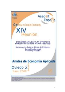
Figure 3: Total export values from Sweden to Germany (in billion SEK) Source: SCB 2011 According to SCB statistics updated in September 2011, Germany is a major exporting partner of Sweden from 2000 until June 2011. In 2010, export value to Germany represented over 10% of total exports of Sweden. The Germany is still the largest and most potential market inside and outside Europe till now. In Berlin on 22nd January 2008, Ewa Björling – Sweden Minister for Trade – emphasized the important role of Germany in Swedish foreign trade and trade policy which was underestimated. Asia are considered to be main markets in the world while Germany is the largest Sweden’s trading partner with higher export values than to all of the 50 Asian countries, including China. Moreover, and perhaps most importantly, Germany is a central political partner in the endeavors to enlarge and deepen Swedish markets. Additionally, in reality, manufacturing of machinery and equipment

21

occupied 44.1% of total Swedish export values in 2010. Consequently it is considered as one of the Swedish largest export items since the end of World War II. Besides, the Figure 3 illustrates the monthly export values from Sweden to Germany from January 2010 to Jun 2011. Although there is an unstable and fluctuated movement of export values during period above, the overall picture still shows an obviously slight increase in the total export value during both period of 2000:2008 and 2008:2011 separately. From 2000 to 2002, Germany used both euro and German mark, denoted DEM, which was converted to euro with the rate of 1.95583 fixed in December 2008 by European Commission. At this time, Swedish exports of goods amounted to around SEK 7 billion in average each month. Comparing to later period from 2002 when Germany started using euro as their official currency, the export went up continuously in value due to either of some changing in trade policy such as tariff, quota, etc. or supporting programs between all members in European Union. The peak value was up to SEK 11.5 billion in the middle of 2008 then dropped dramatically in 2009. From the early 1990s until 2008, Sweden enjoyed a sustained economic upswing fueled by strong exports and rising domestic demand. In the fourth quarter of 2008, Sweden entered a recession. Main export industries of Sweden are autos, telecommunications, construction equipment, and other investment goods. Consequently, there was a sharp decrease in external demand of Sweden due to the economic crisis. According to several economists, compared to Germany and other European countries using euro, the Swedish currency (SEK) was suggested a relatively short recession. From 2010 up to now, the Swedish economy has started to recover with 5.5% increasing in GDP in comparison to the previous year. The strong public sector finances and a reliable exportdriven economy are the main-driven factor for this rising. In this period, the main Swedish exports include machinery and transport equipment, chemical and rubber products, food, clothing, textiles and furniture, and wood products. Exports and investments have been 22

rapidly increasing, and the Swedish export to Germany reached a number of nearly 11 billion kronor in May 2011.

4.2. Bilateral exchange rate 4.2.1. Swedish krona and euro Sweden used krona noted SEK as its official currency as a result of the fact that Scandinavian Monetary Union came into effect in 1873. Regarding the euro, it came into existence on 1 January 1999 and became popular in all European Union member countries including Germany. Sweden joined the European Union in 1995 but the country stayed out of euro. Considering when joining the European Economic and Monetary Union (EMU), J. James Reade & Ulrich Volz (2009) conclude that

the costs and benefits of Sweden, a small

economic market, will lose at least in term of monetary dependence. Moreover, in the 1990s crisis, politicians aimed for stability and therefore tried to keep the exchange rate steady. The attempt failed miserably, and the krona was allowed to float ever since. Since November 1992, the exchange rate of Swedish krona has been officially made floating; this decision has affected greatly the monetary policy in Sweden until now. In spite of the uncertainty that the flexible exchange rate creates in the economy, Swedish government still expect to reach the long term price stability in both of fiscal and monetary policy (Bengt Dennis et al., 1992). As the result of Swedish krona depreciation after the floating free decision, the comparativeness of Swedish industry has improved, and it slows down further decline in the economy. The price of the krona, or the exchange rate, drops then makes Swedish products cheaper for foreigners. Further information of euro is provided in the current paragraph. The euro is implemented with the goal of creating an European economy stability. Looking back at the history of euro, the euro helped improve economic growth across Europe and offered more 23

integration among financial markets. Besides, the euro currency not only strengthens European presence in the global economy through being a reserve currency but also helps ease exchange rate volatility among different European nations. 4.2.2. Exchange rate measurement There is no big concern among researchers on whether nominal or real exchange rate should be used for independent variable and exchange rate volatility measurement. In earlier studies, the group of researchers refer to use the nominal exchange rate (see Hooper & Kohlhagen, 1978; J. G. Thursby & Thursby, 1987) while in recent researches, real exchange rate is used most frequently (McKenzie, 1999; Qian & Varangis, 1994 for example). Bini-Smaghi (1991) points out that the nominal series better capture the volatility driving the uncertainty faced by exporters. The opposite opinions come from Gotur (1985) and Silvana Tenreyro (2003), they argue that the real exchange rate is the most appropriate measure. However, there are no big differences in results of using nominal or real exchange rate measurement (Huchet-Bourdon, M. and J. Korinek, 2011), hence real exchange rate is used in my paper. The real exchange rate is then equal to the nominal exchange rate, multiplied by differences in price levels. Consumer price indexes (CPI) of both Sweden and Germany are used to convert nominal exchange rates into real exchange rates as following formula: Real ER = Nominal ER * CPI Germany / CPI Sweden

24

4.2.3. Exchange rate movement 11.5 Nomality ER Real ER

11

10.5

10

9.5

9

8.5

8 2000

2002

2004

2006

2008

2010

Figure 4: Nominal and real exchange rate development Source: OECD 2011 Based on actual data plotted in the figure 4, the gap between nominal and real exchange rate values is not too high and their patterns are generally similar to each other during 2000 and mid of 2011. The real krona-euro exchange rate movement reflects the depreciation or appreciation of Swedish krona against euro. During 2000:2002, after the euro was established in January 1999, a devaluation of Swedish krona relative to euro was characterized. Since then, the trend tended to be stable during next 6 years up to the second half of 2008. The exchange rate values moved around 9 and 9.4 per euro. Due to the impacts of world financial crisis from 4th quarter 2008 and the Riksbank’s reduction of the interest rate, the euro rapidly appreciated against the Swedish krona by 20% from nearly 9.5 kronor per euro in Sep 2008 to around 11.1 kronor per euro in Mar 2009. According to those figures, this is the worst performance of Swedish economy since 1940 (Peter Garnham, 2009). Later on, in the second half of 2009 and early 2010, the krona started to appreciate then during late 2010 and early

25

2011 it continued to appreciate at a quicker rate. The exchange rate is currently between 8.5-9 kronor per euro.

4.3. Exchange rate volatility 4.3.1. Exchange rate volatility measurement A number of measures of exchange rate volatility have represented for uncertainty and there is no consensus about the appropriateness of one measure relative to others (Huchet-Bourdon, M. and J. Korinek, 2011). The present theoretical analysis has considered three different measures of exchange rate volatility: 

“a short run measure of volatility defined as a 12-month rolling window of the standard deviation in the past monthly real exchange rate” (Bahmani-Oskooee & Wang, n.d.; Mohsen Bahmani-Oskooee & Massomeh Hajilee, 2011; Mohsen Bahmani-Oskooee & Rajarshi Mitra, 2008a)



“a similarly defined measure over 5 years to obtain a long run measure of volatility” (e.g. Huchet-Bourdon, M. and J. Korinek, 2011), and



“a conditional volatility measure estimated from a GARCH mode”l (e.g. Doyle E., 2001). A moving standard deviation over 12 months method has commonly been used in

previous studies (Huchet-Bourdon, M. and J. Korinek, 2011). For each month, this measure is the standard deviation of previous 12 observations ending that current month in the first case. Only empirical results based on 12-month standard deviation are reported in my paper.

26

4.3.2. Exchange rate volatility movement The Swedish krona-euro rate volatility against time is plotted in order to check if volatility is higher around times of sharp appreciations of currencies than it is around times of sharp depreciations. The figure 4 shows that volatility of the real Swedish krona-euro exchange rate was very high around the time of the sharp Swedish krona depreciation between September 2008 and March 2009. The next largest monthly krona appreciations over this period occurred from October 2009 up to the end of 2010. In both cases, real volatility jumped, but not to the unusual extent. Moreover, during the period of 2002 to early 2008, volatility changed little because the magnitude of the Swedish krona appreciation or appreciation against euro was not particularly large. No spike in volatility with the most recent months of 2011 is noted due to stable Swedish and European economies. 0.8

0.7

0.6

Vol

0.5

0.4

0.3

0.2

0.1

0 2002

2004

2006

2008

2010

Figure 5: Evolution of the exchange rate volatility defined as the first method: 12-month rolling window of the standard deviation in the past monthly real exchange rate

27

5. Econometric Methodology The results from equation with the ordinary least squares (OLS) method reveal how much each independent variable influences the dependent variable. Yt and Xt are used as the dependent and independent variable respectively in the following sample model: =

+

+

(1)

The equation (1) is considered as the long run model. In order to find the long run relationship existence by implementing the bounds testing procedure, modeling equation (1) is used as a conditional Auto Regressive Distributed Lag (ARDL) Model: ∆

=

+∑

∆

+∑

∆

+

+

+

(2)

Where c0 is drift component, and ut are white noise errors. This technique suggested by Pesaran, Shin, & Smith (2001) is used for investigating long run relationship between variables based on F-tests or t-tests standard. One more important thing in this technique, they ruled out pre-unit-root testing. The time series data can be stationary I(0), integrated of order one I(1) or mutually co-integrated. This is one of the main advantages of the bounds testing approach because the main variable could be stationary whereas others variables could be non-stationary (Mohsen Bahmani-Oskooee & Rajarshi Mitra, 2008b). This approach is adopted from two main past approaches shown by Engle & Granger (1987) and Johansen (1995) who assume that the variables are integrated of order one I(1) or more. Besides that, following Harris & Sollis (2003), this method provides an unbiased estimation of the long run model and valid t-value even if some of the regressors are endogenous. Finally, the bounds test approach inherits a property that the short run and the long run effects are inferred from the same model.

28

In equation (2), the short run effects are inferred from the estimates of

1

and

2

and

long run effects by the estimate µ2 which is normalized on µ1. A linear combination of the lagged level of all variables, including in equation (2), is commonly referred to an error correction term. Estimating the ARDL model is the first step to carry out either the F test for joining significances of the lag level variables or t-test for the null hypothesis H0: µ1=0. However, many studies including Bahmani-Oskooee & Ardalani (2006) have shown that the F test will be sensitive to the order of lags, thus the choice of lag length is related to important task in the first step. Pesaran et al., (2001) suggests imposing a fixed number of lags on each first differenced variable and using Akaike’s Information Criterion (AIC) to select the optimum lags on each variable. In this paper, different ARDL models are initially estimated for all lags with a maximum of 4 lags by the OLS method, same with proposal of Bahmani-Oskooee & Tankui (2008). With the optimal lags, the F-test (so that H0 : µ1=µ2=0) or t-test (so that H0 : µ1=0) is carried out to investigate the presence of co-integration. Those two separate familiar statistics are employed to the bounds test with new critical values, which are proposed by Pesaran et al. (2001). Two asymptotic critical value bounds provide a test for co-integration when the independent variables are I(d) (where 0 ≤ d ≤1) (see more De Vita & Abbott, 2002). A lower critical value is established by assuming all regressors to be stationary or I(0), and an upper one is established by assuming all variables to be integrated of order one or I(1). If test statistics are located above the respective upper critical values, the existence of a long run relationship will be concluded. If the test statistics fall below the lower critical values, the null hypothesis of no co-integration will be not rejected. Lastly, if the statistics fall within their respective bounds, inference would be inconclusive.

29

In the second step, after confirmation of co-integration existence among those variables in equation (2), the long run and short run model can be derived. Estimation of conditional long run coefficients in equation (1) can be obtained by following formulas (Pesaran, 1999) = -c0/π1 = - π2/π1 Estimate of π1 is used to form an error correction term, say, ECMt-1. When all variables are adjusted toward their long run equilibrium, the gap between the dependent and the independent variables measured by the coefficient associated to ECMt-1 must decrease. In other words, a negative and significant coefficient obtained for ECMt-1 will not only be an indication of adjustment toward equilibrium but also an alternative way of supporting cointegration among variables. The adjustment parameter in absolute value lies between zero and one. The larger the error correction coefficient is, the faster is the economy’s return to its equilibrium after a shock (Huchet-Bourdon, M. and J. Korinek, 2011). Finally, running various diagnostic tests is an important step to detect econometric problems in chosen models. Following previous researches (e.g. Bahmani-Oskooee & Marzieh Bolhasani, 2011; Bahmani-Oskooee & Scott W. Hegerty, 2007; Bahmani-Oskooee & Zohre Ardalani, 2006), the Lagrange Multiplier (LM) statistic to test for non autocorrelation of residuals, the Ramsey’s RESET test for functional misspecification and the Breusch-Pagan test for heteroskedasticity are produced. In addition, to test the stability of short run and long run coefficient estimates, CUSUM and CUSUMSQ tests proposed by Brown, Durbin, & Evans (1975) to the residuals of the error-correction models are applied.

30

6. Econometric Modeling To access the impact of exchange rate variability on Swedish’s export or Germany’s import value, following the previous studies (e.g. Bahmani-Oskooee & Payesteh, 1993; Kenen & Rodrik, 1986), mathematically, the export long run model is formulated as log-linear form in the below equation: =

+

,

+

+

+

,

(3)

Where Xi is the total and 10 biggest groups of commodities export values from Sweden to Germany, IPI is Germany’s real income which is represented by Germany’s industrial production index, ER is for the real bilateral exchange rate, Vol is the measure of exchange rate volatility and Ɛi is an error term. All variables are taken in logarithm forms which allow estimating of elasticity. From the given specifications of equation above, a positive estimation of α1, imply that an increase in Germany’s income or output is considered to boost Germany’s import, is expected. In the opposite point of view, in case of the increasing production of import substitute goods, a decline of Germany import will lead to a decrease in Swedish export, hence a negative sign is estimated

for

α1.

Besides,

a

real

depreciation/appreciation

of

the

euro

(appreciation/depreciation of Swedish krona), reflected by a decrease/increase in real exchange rate, is to lower/boost the Sweden export value. That means the estimate of α2 should be positive. Finally, an estimate of α 3 can be negative or positive depending on whether an increase in the measure of exchange rate sensitivity is to hurt or boost the Sweden exports of commodity i.

31

The estimates of α1- α 3 coefficients would yield the long run effects of the right-hand side variables on the dependent variable. In effort of inferring the short run impacts, long run model should be expressed in an error-correction modeling format as in the equation (4): ∆

= +∑

∑

∆ ∆





+ ∑

,

∆

+

+∑

∆

+

+

,

+

,

,

+

+

,

(4)

(Huchet-Bourdon, M. and J. Korinek, 2011; Mohsen Bahmani-Oskooee & Massomeh Hajilee, 2011 for instance) In equation (4), the short run impacts on export values are inferred by the estimates of −

d 1k – d4k, and estimates of

divided by

reflect the long run effects. In particularly,

the long run coefficients in equation (3) are calculated as following formulas:

=

−

;

=

−

;

=

−

;

=

−



The “bounds testing” approach, explained in econometric methodology, is applied in investigating the existence of the long run relationship. As explained earlier in econometric method, the estimate of

or the error correction

coefficient indicates the speed of the adjustment. The export must adjust to restore the long run equilibrium in the market. Moreover, a negative and highly significant error-correction term is a further evidence of the existence of a long run relationship.

32

7. Empirical results 7.1. Stationary Test Before the presence of long run relationship between export volume and three other variables is determined, pre-unit root testing is applied. Needless to check the stationary for application of the “bounds test”, the orders of integration of all time series are still investigated by means of the Augmented Dickey–Fuller (ADF). This is strongly confirmed by the mixture of I(0) and I(1) series found across the whole period, thus the bounds test pointed out by Pesaran, Shin, & Smith (2001) is the most appropriate method in this case. Table 1: Dickey-Fuller (DF) Test

Variables LNEX LNG07 LNG17 LNG19 LNG20 LNG21 LNG24 LNG26 LNG27 LNG28 LNG29 LNER ∆LNER LNVol ∆LNVol LNIPIge

Coefficient Estimates of first lag of each variable Order of tc tct integration -0,199 (-3,845) -0,443 (-6,181) I(0) -0,235 (-4,167) -0,643 (-7,944) I(0) -0,395 (-5,766) -0,534 (-6,986) I(0) -0,629 (-7,865) -0,636 (-7,895) I(0) -0,476 (-6,557) -0,740 (-8,922) I(0) -0,608 (-7,774) -0,840 (-9,853) I(0) -0,222 (-4,065) -0,407 (-5,851) I(0) -0,537 (-7,247) -0,547 (-7,285) I(0) -0,318 (-5,133) -0,734 (-8,722) I(0) -0,305 (-5,013) -0,601 (-7,640) I(0) -0,364 (-5,513) -0,389 (-5,707) I(0) -0,039 (-1,765) -0,045 (-1,547) I(1) -0,796 (-9,377) -0,803 (-9,401) I(0) -0,022 (-1,116) -0,028 (-1,341) I(1) -0,354 (-5,245) -0,356 (-5,243) I(0) -0,413 (-6,030) -0,552 (-7,206) I(0)

Note: tau values are reported in brackets. Subscripts c, and ct denote, respectively, that there is a constant, and a constant and trend term in the regression. 5% critical DICKEY–FULLER is −2.89 for c & -3.45 for tc. This is adapted from table D.7, p975 (Gujarati, 2002)

According to ADF test, the null hypothesis here is non-stationary. It will be rejected if the absolute computed tau-value exceeds the absolute critical one at the chosen significant 33

level and vice versa. As can be seen in Table 1, except the absolute tau statistics of the exchange rate (LNER) and its volatility (LNVol) series, others reported in brackets are bigger than 2.89 in case of including constant; or 3.45 in case of constant and trend in regressions (at 5% significant level). By taking the first differences of non-stationary time series, stationary ones can be obtained. In conclusion, using all actual observations, the results presented in Table 1 indicate that only logarithm of exchange rate and its volatility appear to be integrated of order one or I(1), rest of series are most likely stationary or I(0).

7.2. Optimal lags Table 2:Optimal lags Industry

∆LNXi

Total export 07 Metal ores 17 Paper and paper products 19 Coke and refined petroleum products 20 Chemicals and chemical products 21 Basic pharmaceutical products and pharmaceutical preparations 24 Basic metals 26 Computer, electronic and optical products 27 Electrical equipment 28 Machinery and equipment 29 Motor vehicles, trailers and semi-trailers

∆LNIPI

∆LNER

∆LNVol

AIC

2 2 2 3 1

3 0 3 1 0

3 2 1 0 3

1 0 3 3 3

-337.435 79.41684 -329.828 217.5063 -61.3161

3

1

1

2

-17.7796

2 3 2 3 3

3 1 1 2 2

2 3 3 3 3

2 3 2 1 3

-115.626 -93.08 -171.035 -192.434 -42.9993

As mentioned in econometric methodology, choosing the optimal lags in ARDL-ECM model is an attributed step to run further regressions. Among all considered possible models, the one with the smallest value of Akaike’s Information Criterion (AIC) is chosen as the best model. Corresponding to the smallest AIC values, values of n1, n2, n3 and n4 in equation (4) are determined then the best models with the optimal lags are identified in Table 2.

34

7.3. Short run analysis In this section, the short run estimates of ARDL models using monthly data over the period 2000-2011 from all estimated industries are provided. Starting with the short run coefficient estimates obtained for the exchange rate volatility (∆ln Vol), other variables such as real exchange rate (∆ln ER) and industrial production index (∆ln IPI) are mentioned later. Firstly, after running regression (4), the results in Table 3 (see Appendix) reveal that short run exchange rate volatilities (∆ln Vol) impact export values in most cases but their effects are complicated. Gathering the information from Table 3 there is at least one significant short run coefficient at the 10% level in 8 of 11 investigated cases. To be exact, these eight industries are coded 17, 20, 21, 24, 26, 27, 28 and total export. These cases in which the coefficients are significant, some industries show the positive effects while others show the negative ones. That means these impacts can move in either directions. These results are consistent with other previous studies concluding that short run effects are not likely to follow a specific pattern (Baek & Koo, 2009; Huchet-Bourdon, M. and J. Korinek, 2011 for instance). Furthermore, the 12-month moving standard deviation to construct the volatility suggests that past information is particularly relevant in order to assess the impact of exchange rate volatility on export values. Secondly, for the real exchange rate, same conclusion with exchange rate volatility variable is presented. The real exchange rate is considered as an important factor determining the export earnings of most industries. The results in table 3 also reveal real exchange rate (∆ln ER) carries the significant coefficients (at the 10% significance level) in most of the cases excluding the industry of coke and refined petroleum products (coded 19). Besides, in majority of industries, the estimates of coefficients are positive, implying that a real depreciation of Swedish krona against euro (or increase in value of exchange rate) will boost export from Sweden to Germany because buying goods from Sweden becomes cheaper for 35

consumers in Germany market. This finding is different with J-curve effect which explains that after a real depreciation, the export values do not change in short run because the exchange rate in current trading contract is already fixed. As for the effects of industrial production index (proxy for Germany income), consistent with many econometric studies, this variable (∆ln IPI) is highly significant in almost cases except for industry of metal ores (coded 07). It means that the foreign income plays an important role in determining domestic exports.

7.4. Long run analysis 7.4.1. Co-integration analysis However, whether these short run effects last in the long run is another big concern in this paper. Following the “bounds test” approach, F-test or t-test can be applied to test the long run relationship. The null hypothesis which is no co-integration will be rejected if the estimated F or t statistic is located above the upper critical value at integrated of order one I(1). This result suggests a long run relationship between 3 independent variables and export values. In other words, the long run results in Table 4 (see Appendix) would be valid if co-integration among the variables is supported either by the F-statistic or by a negative and significant ECMt-1 (tstatistic). Therefore, the long run coefficients’ estimates are indeed meaningful. In actual cases, for the F-test: H0 :

=

=

=

=0

H1 :

≠

≠

≠

≠0

According to F-value shown in table 5 (see Appendix), in the majority of cases, the computed F-statistics at optimal lag are greater than 3.77 which is the upper critical value at 10% level of significance. 7 of total 11 investigated cases (coded 07, 17, 20, 24, 27, 28 and 36

total export) indicate a long run relationship between Germany income, exchange rate, its volatility and export values. For the t-test (checking the negative and significant of ECMt-1 coefficient): H0 :

=0

H1 :