Financial Markets and Instruments FIN 3560 – 01 Professor Michael A. Goldstein, PH.D.
The Effect of Interest Rates on the Euro’s Foreign Exchange Rate
Andrea Canavesio Joseph Hage Chahine Felipe Piedrahita
I
12/5/2011
Table of Contents: Executive Summary…………………………………………………………………………………………………………………………………… Background of the Euro……………………………………………………………………………………………………………………………1 Brief history of the European Union and the Euro……………………………………………………………………….1 The Monetary Snake…………………………………………………………………………………………………….…………….1 The European Monetary System…………………………………………………………………………………….…………..2 The Exchange Rate Mechanism……………………………………………………………………………………….………….3 Euro Convergence Criteria…………………………………………………………………………………………………………..4 Current European Debt Crisis……………………………………………………………………………………………………………………5 Foreign Exchange Rates Theory……………………………………………………………………………………………………….………7 Short-run Exchange Rates…………………………………………………………………………………………………….…….7 Long-run Exchange Rates….………………………………………………………………………………………………………..8 Purpose of Analysis………………………………………………………………………………………………………………….…8 Variables…………………………………………………………………………………………………………………………………….9 EURIBOR………………………………………………………………………………………………………………….……..9 LIBOR……………………………………………………………………………………………………………………..………9 Federal Funds Rate……………………………………………………………………………………………….………..9 Inflation – Real and Expected …………………………………………………………………………………………9 GDP Growth………………………………………………………………………………………………………………….10 Analysis of the Euro-US Dollar exchange rate…………………………………………………………………………………………10 Analysis of Assumptions……………………………………………………………………………………………………………10 P-value…………………………………………………………………………………………………………………………10 1999 – 2011……………………………………………………………………………………………………………………………...11 Best fit………………………………………………………………………………………………………………………….11 Interest rates………………………………………………………………………………………………………………..11
Simple regressions……………………………………………………………………………………………………..…12 2000 – 2006 …………………………………………………………………………………………………………………………..…13 Best fit……………………………………………………………………………………………………………………….…13 Interest rates………………………………………………………………………………………………………………..13 Simple regressions………………………………………………………………………………………………………..14 2007 – 2011………………………………………………………………………………………………………………………………15 Best fit……………………………………………………………………………………………………………………….…15 Interest rates………………………………………………………………………………………………………………..15 Simple regressions……………………………………………………………………………………………………..…16 Conclusion………………………………………………………………………………………………………………………………………….….17 References………………………………………………………………………………………………………………………………………..……18 Exhibits……………………………………………………………………………………………………………………………………………….…19 Regression Outputs………………………………………………………………………………………………………………………………..21 1999 – 2011………………………………………………………………………………………………………………………………21 Simple regressions………………………………………………………………………………………………………..21 Multiple regressions……………………………………………………………………………………………………..23 2000 – 2006………………………………………………………………………………………………………………………………26 Simple regressions………………………………………………………………………………………………………..26 Multiple regressions……………………………………………………………………………………………………..28 2007 – 2011………………………………………………………………………………………………………………………………31 Simple regressions………………………………………………………………………………………………………..31 Multiple regressions…………………………………………………………………………………………………..…33
Executive Summary: In analyzing the Euro we have decided to focus on its history, theory behind short-run and longrun foreign exchange rates, and the factors that affect the foreign exchange rate of the Euro. History has provided us with a basis of understanding as to how the Euro has affected the economy of the Euro zone and it has shown us what the purpose of the creation of this currency was. In order to perform our analysis we also had to have a general understanding of how exactly foreign exchange rates are determined and what are the factors affecting changes in these rates. The purpose of our analysis was to determine if the theory behind foreign exchange rates holds true and to what extent do the variables that theoretically affect exchange rates actually affect them. Along with our analysis of how the theory behind foreign exchange rates holds in the real world we will also be looking at why the Euro is valued higher than Dollar even though the Euro zone economy is in worse shape than the American economy. Analysis of the variables that theoretically affect foreign exchange rates should provide us with an answer as to why the EUR-USD exchange rate has been behaving this way. The variables we believe are the equivalents of EUR-USD exchange rates according to theory are LIBOR, EURIBOR, the Federal Funds rate, Euro zone inflation and Euro zone GDP growth. In order to analyze the effect of each of these variables on the EUR-USD exchange rate we have run several regressions. These regressions have provided us with an answer as to what has the most significant factors of these foreign exchange rates. Our belief is that the Euro is valued higher than the US Dollar because interest rates are much higher than in the US. We believe these higher interest rates are much more attractive to foreign investors. This causes foreign investors to demand the Euro in the foreign exchange market which in turn leads to its appreciation. Through our analysis we will be able to determine if our hypothesis is correct.
Background on the Euro Brief history of the European Union and the Euro The European Union along with the Euro’s conception can be traced back to the founding of the European Community in 1967, an entity comprising of the three main economic pillars of Europe at the time: the European Atomic Energy community, the European Economic Market, and the European Coal and Steel Community. In point of fact, the driving factor behind the creation of the EU was a political move aimed at creating an economic interdependence between European countries, particularly France and Germany, in order to avoid future wars given the disastrous consequences of World War II1. The European Economic Market laid ground for the European Monetary System (EMS) which aimed to create an integrative economic system by eliminating trade barriers, promoting fiscal integration, and reducing trade hindrances related to currency exchange rates fluctuations. By doing this, the EMS would be able to sustain European monetary stability, resulting in the creation of the European Currency Unit (ECU). Even though the ECU was not a currency in circulation, it had clear diversification advantages for foreign investors, particularly since the Bretton Woods Agreement ended the convertibility of the US dollar to gold in 1971 2. The Maastricht Treaty signed in 1992 led to the creation of the formal European Union, constituted of the euro zone and its anteroom, the European Exchange Rate Mechanism (ERM). The ERM’s long term role was to stabilize exchange rates among members of the euro zone and assist in the convergence of their economies in view of the upcoming integration of a unique currency, the Euro. On January 1st 1999, the Euro officially replaced the European Currency Unit at par, 1 Euro being equal to 1 ECU. However, it was not until 2002 that the Euro came into circulation under its fiduciary form. The Monetary Snake Recognizing the fact that they were not only mutual clients, but major reciprocal suppliers as well; Western European countries created the Snake in the Tunnel policy in 1972 in order to strengthen and protect the economic interests that tied them to one another. These countries realized their commercial trades were vulnerable to volatile exchange rates, and could be the target of speculation. The various European currencies involved were able to move ±2.25% relative to their central rate 1
Marc Levine, Francis Kim, and Joel Siegel. The CPA Journal, April 1999 2 Ibid
1
against the US dollar, thus creating a narrow band of fluctuation for the participating currencies, the Tunnel being the US dollar. However, European currencies had fluctuation margins of ±4.5% among one another in relation to the US dollar, and the ever expanding leniency of the bands ultimately brought the Tunnel to collapse 3. Since its very beginning, the economic turmoil from 1972 to 1978 proved the Monetary Snake to be unsustainable. The British Pound had to be withdrawn from the Snake a month after entering it, and never made a comeback, destabilized by the 1973 oil crisis and later hit by the 1976 Sterling crisis. Merely a year after its entry to the Snake in 1973, the Italian Lira had to exit, followed by the French Franc in 1974, and again later in 1976. By 1977, the Deutsche Mark was still following the Snake and dominating the Tunnel, and only three other currencies were able to keep up with the constraints. The necessity to elaborate a new monetary system was clear; a system that would prevent the Deutsche Mark from rising too high by weighting it to the weaker currencies of Germanys’ economic partners 4. The European Monetary System: The European Monetary System (EMS) was introduced in 1979 after the notable failure of the Snake in the Tunnel policy. The EMS brought two main technical modifications building on the malfunctions of the Snake. First, instead of referring to the US Dollar, the currencies of the new system would use the newly created European Currency Unit (ECU) as a benchmark. The ECU was comprised of a weighted basket of currencies determined by the economic size of each participating EC member. Members of the EC could deposit gold and dollar reserves with the European Cooperation Fund for issuance of ECU currency, except for Greece which did not participate in the EMS exchange rate system. This currency composite was used as a reserve unit, an accounting unit, and a unit of settlement for the EMS central banks 5. Second, since the fluctuation of currencies against one another appeared to be untenable, the new variation of ±2.25% (or 1.125 % on either side of the parity exchange rate) would be relative to the basket. Each currency was then expected to float against the average of the other currencies, even though this system allowed room for maneuver since every Central Bank could intervene on its currency as it approached one of the boundaries.
3
Nicholas Moussis. The 1971 Resolution. 4 European Parliament. The historical development of monetary integration. 5 Marc Levine.
2
Nonetheless, one should keep in mind the ECU was not a common currency, but a mere financial instrument deducted daily from the exchange rates of the participating EC members. Given its status of financial instrument, the ECU could also be potentially subject to speculation. In 1992 for example, the Italian Lira and Spanish Peseta are devalued due to speculations on the markets, and the British Pound is forced to withdraw from the EMS by the speculative hedge fund manager George Soros, who massively shorted the Pound believing the UK government would be reluctant to raise its interest rates to the levels required by the EMS. Furthermore in 1993, France sustains important speculative attacks on the Franc 6, and is forced to dig very deeply in its monetary reserves to unsustainable levels, which leads to the establishment of a new fluctuation band of ±15%. The Exchange Rate Mechanism As part of the newly created European Monetary System, the EC introduced the European Exchange Rate Mechanism to stabilize the various European currencies’ rates and soothe the risks associated with currency exchange. In the long run, the ERM was aimed at attenuating inflation and stimulate the economic trades within the European Community zone, in order to create stability and confidence in view of the upcoming adoption of a unique currency. This Exchange Rate Mechanism cut short the pattern in which European countries used to voluntarily devaluate their currency to stimulate their economy and increase their interest rates to encourage foreign investments. In retrospect, these direct interventions proved to be inefficient and inflationist, whereas the EMS supported the EC nations in need by compensating the necessary devaluation. This was the true beginning of the European economic cooperation, in which finance ministers were to officially meet and EC nations were to actively help one another. However, the EMS’s functions would be partly modified in 1992 with the signature of the Maastricht Treaty, which among other initiatives, laid ground to the creation of a European Central Bank. The institutionalization of the ECB would require a few years, and in the meantime National Central Banks were urged to adopt strict budget policies to sustain the long term economic convergence of the various EC members. This explains why the Exchange Rate Mechanism (ERM) would only prove to be entirely beneficial during the last 2 years of the European Monetary System, in 1998 and 1999. In fact, once the status of the European Central Bank has been fully established in 1998, it led to a definitive period during which the ERM would be useful to evaluate the currencies of the countries that 6
John Eisenhammer. The ERM Crisis: Speculation: Soros Moves in on the Franc. The Independent, July 1993.
3
were about to incorporate the Euro 7. Even if the initial purpose of the ERM was somewhat altered given the circumstances, it assisted the European countries in their accession to the upcoming unique currency. Euro Convergence Criteria The aforementioned economic measures integrated among members of the EC would ultimately lead to the creation of the European Union through a series of steps meticulously orchestrated to unfold into a single currency, the Euro. This last step, referred to as the Maastricht Criteria, consists in a series of economic convergence measures that would allow EU members to be on the same economic wavelength in order to integrate the Euro. The Euro Convergence Criteria aim at controlling inflation rates, public debt, public deficit, exchange rates, and long term interest rates, respecting the following characteristics 8: 1. Inflation Rates: should not be greater than 1.5 percentage points above the average of the three best performing members 2. a) Annual Public Debt: the ration of gross government debt to GDP should not exceed 60% at the end of the preceding fiscal year b) Annual Public Deficit: the ration of government deficit to gross GDP should not exceed 3% at the end of the preceding fiscal year 3. Exchange Rates: applicant countries should have joined the ERM II under the EMS for two consecutive years and should not have devalued their currency during that period 4. Long-Term Interest Rates (nominal): should not be more than 2 percentage points above the average of the three lowest inflation member states Following on the footsteps of the Euro Convergence Criteria, members of the European Union that take part in the euro zone adopted the Stability and Growth Pact (SGP) in 1997. The SGP had essentially similar criteria except for adding more flexibility to make the pact more enforceable, while establishing sanctions against countries that deviate excessively. The SGP has never been considered a success and remained fairly discrete on the international scene, since the European Council of Ministers failed to 7
European Commission Eurostat. Exchange Rates and Interest Rates. 8 Europa, Summeries of EU Legislation. Introducing the Euro: Convergence Criteria.
4
apply any sanctions over the years. Punitive measures were undertaken against Portugal in 2002 and Greece in 2005, although sanctions have never been enforced. Same applies to France and Germany, which benefited from their political authority and economic dominance to avoid any sanctions. In 2011 and following the 2010 sovereign debt crisis, the Euro Plus Pact was created as a successor to the SGP, with more stringent rules aimed at reinforcing the competitiveness of the euro zone countries. Nonetheless, the maximum amount of public deficit caped at 3% might be difficult to justify from an economic standpoint, since the criteria that aim to stabilize public deficit are directly related to the debt’s Primary Deficit (which is equal to the Fiscal Deficit – Interest Payments). Therefore, a fixed ceiling of 3% for public deficit does not make economic sense since growth rates and bond rates are variable from one year to another. For instance, Italy reduced its amount of debt while having a public deficit superior to 3% in 2003, and increased its amount of debt by having a public deficit inferior to 3% in 2008 9. By 2009, Finland and Luxemburg were the only two euro zone countries able to respect the 3% criterion. Countries such as Greece, Ireland, and Spain, had public deficits even exceeding 10% of their respective GDP during that same period. Current European Debt Crisis The current European Debt Crisis can be attributed to Greece and Ireland in a broad sense. On one hand, the Greek crisis originates from a massive public deficit, and the fear investors and lenders have concerning Greece’s ability to repay its debt along with its interest due. On the other hand, the case of the Irish public debt originates from private debt, used to bail out the financial institutions during the repercussions of the sub-prime crisis and the global banking crisis of 2008. Because of the nature of the Greek public debt, it will be of greater interest to us in this paper, in a sense that we believe the Greek debt crisis represents in fact the Euro crisis, since without the Euro, there would be no crisis. When the Greek socialist party gained access to power in 2009 with the election of Prime Minister Georges Papandreou, it was hard to realize the actual public deficit was in excess of 12%, a much higher figure compared to the official 6% claimed by the previous government. Despite these catastrophic figures, Papandreou maintains a stimulus package of 2.5 Billion Euros, simply delaying the public deficit crisis to 2011. Investors and lenders were not fooled, and their confidence in Greece’s 9
Monica Issar. Italy – An Atypical Peripheral Country. JP Morgan Asset Management.
5
ability to repay its debt crumbled, further supported by its notes’ downgrade from the various credit rating agencies. The downgrade in rating raised the interest rates at which Greece was able to borrow money, sending Greece on a downward spiral. In May 2010, the European Union formally agreed on a safety plan for Greece consisting of 110 Billion Euros in lending distributed over 3 years, along with austerity measures that would help Greece save up to 30 Billion Euros (10% reductions in public salaries, reform of their pension plan). This plan seemed like a well perceived measure until the Greek people protested and didn’t seem contented by the austerity measures, which again brought down the hopes and confidence of the international community at large, and provoked another market rally. The members of the EU negotiate the new European Financial Stability Facility (FESF) which would be able to borrow as much as 440 Billion Euros on the markets to support the countries at risk of contagion from the Greek crisis, in addition to the 60 Billion Euros of the European Commission and the 250 Billion US dollars provided by the IMF. This fund would primarily provide support to Ireland and Portugal in the first place, possibly extending its reach to Spain and Italy if needs be. Athens vowed to accelerate its privatization program estimated at 50 Billion Euros, and received in return lower interest rates and extended maturities. Alas that was insufficient; Greece’s public deficit decreased to 9.4% in 2010 which is still deemed excessive, and its public debt increased reaching levels above 150% of GDP. Most of the European members, the ECB, and the Greek government, continue to exclude any procedure of debt restructuring, fearing it would cause the collapse of Greek banks due to speculative attacks that would eventually reach the rest of the euro zone. There lies the real problem of the European Debt crisis: what would happen in the event the Greek crisis spreads to other members of the EU, Italy and Spain in particular? Because in the end, the sum of the Greek, Irish, and Portuguese debt combined altogether is not large enough to bring down the French and German Banking system, while the Italian and Spanish debt alone are able to do so 10. That is why the ECB is currently massively purchasing Spanish and Italian bonds, in order to keep their respective bond markets from crumbling, in opposition to simply printing more money. Germany is exercising great political pressure to ensure countries aren’t being bailed-out on printed money, which would hurt the entire euro zone eventually in the long run. In the event the Spanish and Italian bond markets begin to fall apart, the ECB will sooner or later realize it has to print massive amounts of money 10
Robert Wiedemer. The Real Question in the European Debt Crisis.
6
to inject in the market and stabilize the turmoil. The end results would involve printing money one way or another, and it would be in the ECB’s best interest to get the Fed to lend printed money to Europe, through currency swaps for example, considering the repercussions on US banks if the European ones were to be impaired. 11As of November 2011, a program which consists in borrowing money from the Fed through the ECB in exchange for collateral has been further improved. Interest rates were lowered half a percent, and collateral requirements were made much more flexible, thus promoting borrowing money from the Fed. As of December 1st 2011, a Greek bank can borrow money from the Fed cheaper than a US bank can.12As Robert Wiedemer puts it in his article, “yesterday’s historic breakthrough is now, well, yesterday’s news”.
Foreign Exchange Rates Theory Short-run Exchange Rates Currency exchange rates are affected by many different variables in short-run. The main determinant of the exchange rate of one currency versus another is the difference in prices of financial assets in each of the compared countries. Differences in the price of a domestic financial asset compared to the price of a similar foreign financial asset tend to cause appreciation or depreciation of currencies 13. Investors will compare the two similar financial assets and determine which one will give them the best return while taking into account future fluctuations in exchange rates. The financial asset that is expected to give best return will be the most demanded. The currency of the asset that gives the best return is the one that will be the most demanded. Increased demand for a currency will lead it to appreciate versus the currency of the asset that gives a lower return. Another very important factor that affects foreign exchange rates is interest rates. Interest rates are a function of expected real rates of interest and expected inflation. 𝑛 = 𝑖𝑒 + 𝜋𝑒
Interest rates are very important in exchange rates because they are one aspect investors consider when considering an investment opportunity. The higher the interest rate the more attractive the opportunity is to an investor because they will get a higher return. Investors will demand more of a
11
Ibid Ibid 13 Hubbard, R. Glenn. "The Foreign-Exchange Market and Exchange Rates." Money, the Financial System, and the Economy. Boston: Pearson Addison-Wesley, 2007. Print. 12
7
currency where interest rates are higher and this increased demand will cause that country’s currency to appreciate. For example, in 2002 Euro zone short-term rates rose relative to the US leading the Euro to appreciate against the US Dollar 14. Monetary policy is also very important when considering exchange rates. In the short-run, according to uncovered interest rate parity, tightening of monetary policy will cause a currency to appreciate and loosening of monetary will cause a currency to depreciate 15. Tight monetary policy will lead to higher interest rates in order to discourage borrowing and in turn these higher rates will be more attractive to foreign investors causing them to demand the domestic currency. Loose monetary policy will cause the opposite to occur. Long-run Exchange Rates Over the longer-term there are other factors that affect foreign exchange rates. These include productivity and exports. A country’s productivity is very important to take into account. As a country increases productivity prices will fall because of more efficient manufacturing methods and can produce goods for less; this fall in prices will lead to increased demands for its exports. In order to purchase exports buyers have to purchase that country’s currency. The increased demand for the currency will lead to its appreciation. Consumer preferences for domestic versus foreign goods will also a country’s exchange rate because of the effect these preferences will have on the demand for the domestic currency of the product. 16 Purpose of Analysis Considering what we believe are the most important factors that theoretically affect foreign exchange rates (interest rates, inflation and GDP growth) we have decided to focus on the equivalents of these rates for the EUR-USD exchange rate: the EURIBOR, LIBOR, Federal Funds Rate, Euro zone inflation and Euro zone GDP growth. If theory holds true we expect to find significant correlation between all of these variables and the EUR-USD exchange rate.
14
Ibid. Hubbard. 16 Ibid. 15
8
EURIBOR The EURIBOR (Euro Interbank Offered Rate) is the rate at which banks lend unsecured funds to each other in the Euro zone. This rate is used as a base for interest rates on many other financial products in the Euro zone. We have decided to use this because we believe it is the key interest rate that has an effect on the Euro. Changes in this rate affect the demand for the Euro in the foreign exchange market and can therefore lead to its appreciation or depreciation 17. LIBOR LIBOR (London Interbank Offered Rate) is the rate at which banks in London lend to each other for short periods of time. This rate is also used internationally, including in the US, as a base to determine other short-term interest rates (i.e. some loans are made at LIBOR plus a certain amount of points). Since this rate is frequently used in the US we believe it provides a good comparison to the difference of rates between the US and the Euro zone’s EURIBOR 18. Federal Funds Rate The Federal Funds rate is the rate at which banks in the US lend each other funds at the Federal Reserve overnight. We have decided to include this rate because although it is not used as a base for other financial instruments in the US it does directly affect the interest rates banking institutions decide offer their clients on checkable deposits, demand deposits and other financial instruments 19. Inflation – Real and Expected The Euro zone’s rate of inflation is a very important factor to be considered in the evaluation of EUR-USD exchange rate. As inflation increases nominal rates increase making returns more attractive for foreign investors. This will increase the demand for the currency and lead to its appreciation. Expectations of inflation can also significantly affect a currency’s exchange rate because as more
17
" About Euribor®." Euribor-EBF | Home. Web. 27 Nov. 2011. . 18 "London Interbank Offered Rate (LIBOR)." Investopedia.com. Web. 02 Dec. 2011. . 19 Investopedia.
9
inflation is expected the less that currency will demanded since its purchasing power will fall. This will lead to its depreciation. The opposite tends to occur when expectations of inflation fall. GDP Growth (Productivity) We have decided to include GDP growth of the Euro zone in our analysis because it is a major factor in the area’s rate of inflation. As GDP increases inflation tends to increase and central banks intervene and increase key interest which will then lead to increases in nominal interest rates, which as mentioned before, will make returns more attractive for foreign investors. Analysis of the Euro-US Dollar exchange rate Analysis of Assumptions Our analysis of the Euro–US Dollar exchange rate is based on quarterly data from three different time periods: 1999 to 2011, 2000 to 2006, and 2006 to 2008. The rationale behind this separation is to assess how crises affect the exchange rate’s correlation to different rates. We determined this separation by looking at plots of some of the data we collected (inflation, GDP growth, Federal Funds Rate), and confirming that these rates in 1999, 2007, 2008, 2009, appeared to be outliers (Exhibit 1). For our analysis, the benchmark for the three periods is the multiple regression between the Euro–US Dollar exchange rate and all of the data that we collected (inflation, GDP growth, Federal Funds rate, Euribor, Libor) which we will refer to as base rates. Additionally, we have studied the individual relationship between the base rates and the exchange rate. P-value As you may notice from the regression outputs in the exhibits, some variables in the regressions may have p-values greater than 0.1, which may mean that the regression is not significant enough. Therefore, we tested all of our regressions without these variables, and noticed that correlation dropped. Statistically, this means that the removed variables actually had significance, and therefore that the first regression was valid.
10
1999 - 2011 R2 (adjusted)
Variables
Multiple
Libor 1 FFR
Inflation
GDP Growth FFR
Euribor 1 Inflation GDP Growth FFR Euribor 1 Euribor 1 Euribor 3 Euribor 6 Euribor 12 Libor 1 Euribor 1 Euribor 3 Euribor 6 Euribor 12 Libor 1
P-value (< 0.1) P-value (>0.1)
Inflation Libor 3 Euribor 1 Euribor 3 Euribor 3 Libor 3 Libor 3
Euribor 6 GDP Growth Libor 6 Euribor 3 Euribor 1 Euribor 6 Euribor 6 Libor 6 Libor 6
Euribor 12 FFR Libor 12 Libor 1 Euribor 3 Euribor 12 Euribor 12 Libor 12 Libor 12
Average R2 (adjusted)
11.5% 13.4% 37.2% 52.7% 53.1% 55.4% 69.4% 69.8% 76.5% 48.8%
Table 1.1 – Multiple Regressions, 1999-2011 Best fit Table 1.1 shows the variables and the correlation for the regressions that we ran on the past twelve years of data (1999-2011). As you can see, R-Squared adjusted, which measures correlation, tends to increase with the number of variables that the regression takes into account. The regression that records the highest level of correlation, specifically 76.5%, is the one that includes all of the base rates. Therefore, the combination of these rates accounts for 76.5% of the variation in the currency exchange rate. Interest rates The analysis shows that the Euro-US Dollar exchange rate is mostly affected by the Euribor (R-sq adj. 55.4%) rather than the Libor (R-sq adj. 37.2%). Additionally, the shorter-term Euribor (1-month, 3month) have a higher correlation to the Euro compared to the relatively longer-term Euribor (6-month, 12-month). R-Squared adjusted for the one and three-month Euribor is 53.1%, whereas R-Squared adjusted for the six and twelve-month Euribor is only 11.5%.
11
Simple Regressions
Simple
Variables Inflation Euribor 12 GDP Growth Euribor 6 Libor 6 Euribor 3 Libor 3 Libor 12 Libor 1 Euribor 1 FFR
R2 0.1% 8.7% 9.5% 10.2% 11.9% 12.3% 12.8% 13.3% 14.3% 17.4% 17.4%
Low p-value (< 0.1) High p-value (>0.1)
Table 1.2 – Simple regressions, 1999-2011
As we can see from table 1.2, all of our base rates have a low correlation to the exchange rate. This data tells us that, individually, our base rates can explain less than 20% of the Euro’s variations. Nonetheless, we ran these regressions to understand which factors had the most significance in the Euro-US Dollar exchange rate. Based on the past 12 years of data, therefore including the recent crisis, the Federal Funds Rate and the 1-month Euribor have the highest R2 (17.4%), followed by the 1-month Libor (R2 14.3%). Therefore, very short-term interest rates have the highest correlation to the Euro.
12
2000-2006
Multiple
Inflation
R2 (adjusted)
Variables
GDP Growth FFR
Inflation GDP Growth Euribor 6 Libor 1 Libor 3 Libor 6 Euribor 1 Euribor 1 Euribor 3 Euribor 6 Euribor 12 Libor 1 Libor 3 Libor 6 FFR Euribor 1 Euribor 3 Euribor 1 Euribor 3 Euribor 6 Inflation GDP Growth FFR Euribor 1 Euribor 3 Euribor 6 Euribor 1 Euribor 3 Euribor 6 Euribor 12 Libor 1 Libor 3 Libor 6
Low p-value (< 0.1) High p-value (>0.1)
2
FFR Euribor 12 Libor 12 Euribor 3 Libor 12 Libor 1 Euribor 12 Euribor 12 Libor 12
Average R (adjusted)
16.6% 59.8% 70.5% 70.7% 81.8% 82.3% 83.2% 83.6% 87.9% 77.5%
Table 1.3 – Multiple Regressions, 2000-2006 Best fit Table 1.3 shows the variables and the correlation for the regressions that we ran on the base rates from 2000 to 2006. Similarly to the previous analysis (1999-2011), R-Squared adjusted tends to increase with the number of variables that the regression takes into account, and the model that records the highest level of correlation (87.5%), is the one that includes all of the base rates. This correlation is significantly higher than the one we calculated for the past twelve years, which amounted to 76.5%. As a result, correlation in crisis years is lower than in stable years. Interest rates The analysis shows that the Euro-US Dollar exchange rate is mostly influenced by the Euribor (83.2%) rather than the Libor (70.5%). Interestingly, both R-Squared adjusted increased considerably compared to the same rates in the previously mentioned time period (Euribor 55.4% to 83.2%, Libor 37.2% to 70.5%). This surge in R-Squared adjusted tells us that correlation between the Euro and interest rates is higher in years of growth than in years of crisis. As the previously analyzed time period, shorter-term Euribor (1-month, 3-month) have a higher correlation to the Euro compared to the relatively longer-term Euribor (6-month, 12-month).
13
Simple regressions
Simple
Variables
R2
GDP Growth Libor 6 Libor 3 Libor 12 Libor 1 Inflation FFR Euribor 12 Euribor 6
0.0% 2.0% 2.2% 2.3% 4.9% 5.5% 5.8% 54.7% 59.5%
Euribor 3 Euribor 1
64.4% 68.0%
Low p-value (< 0.1) High p-value (>0.1)
Table 1.4 – Simple regressions, 2000-2006
As we can see from Table 1.2, the Euribor are the only rates that have a significant correlation to the Euro. R2 for the Euribor varies from 54.7% for the twelve-month rate to 68% for the one-month rate. Therefore, in stable years, individual European interest rates can explain between 54.7% and 68% of the Euro’s variations. As previously stated, correlation between any of the rates we studied and the Euro is higher in periods of economic growth. In fact, it is much higher considering that the Euribor’s R2 in the previous time period were 17.4% for the one-month Euribor, 12.3% for the three-month Euribor, 10.2% for the six-month Euribor, and 8.7% for the twelve-month Euribor.
14
2007-2011 R2 (adjusted)
Variables
Multiple
Libor 1
Libor 3
Inflation Euribor 1 Euribor 3 Inflation GDP Growth FFR
Inflation
GDP Growth FFR
Euribor 1 Euribor 3 Euribor 6 Euribor 1 Euribor 3 Euribor 6
Euribor 1 FFR Euribor 12 Libor 1 Euribor 12 Libor 1
Low p-value (< 0.1) High p-value (>0.1)
Euribor 3 Euribor 1 Libor 3 Libor 3
Libor 6
Libor 12
Euribor 6 GDP Growth Euribor 6 Euribor 1 Euribor 6 Euribor 3 Libor 6 Libor 6
Euribor 12 FFR Euribor 12 Euribor 3 Euribor 12 Libor 1 Libor 12 Libor 12
Average R2 (adjusted)
3.3% 7.2% 17.0% 26.3% 29.0% 35.5% 48.9% 82.2% 90.8% 42.1%
Table 1.5 – Multiple Regressions, 2007-2011 Best fit Table 1.5 shows the variables and the correlation for the regressions that we ran on the base rates from 2007 to 2011. Just like the previously examined regressions, R-Squared adjusted tends to increase with the number of variables that the regression considers, and the model that records the highest level of correlation (90.8%), is the one that includes all of the base rates. This correlation is slightly higher than the one we calculated for the growth years. This datum would seem to disprove our theory that correlation is highest in stable years, but we do not believe this to be the case. Part of our reasoning relates back to our explanation of the p-value. Statistically, if the p-value is greater than 0.1, the regression loses significance unless its correlation drops once the inadequate variables are removed from the model. We accepted elevated p-values in our models as our regressions’ correlations dropped after eliminating certain variables. In this time period, p-values are high relative to the previously analyzed years. Therefore, we believe that our theory still holds true. In any case, as you can see from Table 1.5, Average R-Squared adjusted for these recent years is 42.1%, which is considerably lower than the growth year Average R-Squared adjusted which amounted to 77.5%. Interest rates Table 1.5 shows that the Euro-US Dollar exchange rate is mostly influenced by the Euribor (26.3%) rather than the Libor (3.3%). Once again, correlation for the same rates has decreased from stable years (Euribor 83.2% and Libor 70.5%, 2000-2006), and shorter-term Euribor (1-month and 3month 29%) have a higher correlation to the Euro compared to the relatively longer-term Euribor (6month
and
12-month,
15
7.2%).
Simple regressions
Simply
Variables GDP Growth Libor 12 Libor 6 Libor 3 FFR Libor 1 Euribor 1 Euribor 6 Euribor 3 Euribor 12 Inflation
R2 0.0% 0.3% 0.5% 0.6% 1.0% 1.1% 13.1% 15.2% 15.8% 15.8% 19.4%
Low p-value (< 0.1) High p-value (>0.1)
Table 1.6 – Simple regressions, 2007-2011
As we can see from Table 1.6, the Euribor and Inflation are the only rates that have a significant correlation to the Euro for these years. However, all of the p-values for these regressions are out of the significant range, which make the models lose considerable significance, especially since they are simple regressions. Nonetheless, there is consistency in the correlation of the Euribor, which had the highest R2 in the previous time periods, thus proving that, taken individually, these rates have the most influence over the Euro-US Dollar exchange rate.
16
Conclusion During the completion of this work, we studied the background of the Euro, the theory governing foreign exchange rates and the Euro-US Dollar foreign exchange rate. The purpose of this analysis was to comprehend the rationale behind a high valuation of the Euro-US Dollar rate. In fact, it is our opinion that, considering the worse Euro zone state compared to the US, the Euro should be trading at a significantly lower price level. Ultimately, we believe that higher interest rates in Europe are the main factor maintaining the Euro-US Dollar exchange rate at its elevated current value of 1.3448. Our analysis of the correlation between the Euro-US Dollar exchange rate and our base rates (Inflation, GDP Growth, Federal Funds Rate, Euribor, and Libor) can be summarized in three conclusions. First, average correlation between the exchange rate and our base rates is directly proportional to the European and American economic state: when the economies are in poor shape, average correlation is low (42.1%) compared to growth years (77.5%). Second, regressions become less significant (high pvalues) in crisis years, consequently adding uncertainty to future valuations of the Euro. Finally, the third conclusion relates to our thesis: considering that, currently, Euribor are higher than Libor, the high correlation between the former and the continental currency is proof of the interest rate’s substantial influence on the high valuation of the Euro.
17
References: •
ECB Statistical Data Warehouse. Web. 30 Nov. 2011. .
•
European Commission Eurostat. Exchange Rates and Interest Rates.
•
European Parliament. The historical development of monetary integration.
•
Europa, Summeries of EU Legislation. Introducing the Euro: Convergence Criteria.
•
"FRB: H.15 Release--Selected Interest Rates--Historical Data." Board of Governors of the Federal Reserve System. Web. 27 Nov. 2011. .
•
"Historical Euribor Rates by Year." Euribor-rates.eu. Web. 2 Dec. 2011. .
•
"Historical Exchange Rates." OANDA. Web. 27 Nov. 2011. .
•
John Eisenhammer. The ERM Crisis: Speculation: Soros Moves in on the Franc. The Independent, July 1993.
•
"LIBOR Rates History (Historical)." Prime Rate. Web. 1 Dec. 2011. .
•
Marc Levine, Francis Kim, and Joel Siegel. The CPA Journal, April 1999
•
Monica Issar. Italy – An Atypical Peripheral Country. January 31, 2011. JP Morgan Asset Management.
•
Nicholas Moussis. The 1971 Resolution.
•
Robert Wiedemer. The Real Question in the European Debt Crisis. November 30, 2011.
18
Exhibits Exhibit 1 Time Series Plot of EUR-USD 1.6 1.5
EUR-USD
1.4 1.3 1.2 1.1 1.0 0.9 0.8 Quarter Q1 Q1 Q1 Q1 Q1 Q1 Q1 Q1 Q1 Q1 Q1 Q1 Q1 Year 1999 2000 2001 2002 2003 2004 2005 2006 2007 2008 2009 2010 2011
Exhibit 2 Time Series Plot of Spread 1-mo, Spread 3-mo, Spread 6-mo, ... Variable Spread 1-mo Spread 3-mo Spread 6-mo Spread 12-mo
2 1
Data
0 -1 -2 -3 -4 Quarter Year
Q1 Q1 Q1 Q1 Q1 Q1 Q1 Q1 Q1 Q1 Q1 Q1 Q1 1999 2000 2001 2002 2003 2004 2005 2006 2007 2008 2009 2010 2011
19
Exhibit 3 Time Series Plot of Inflation, GDP Growth, Fed Funds Rate 0.075
Variable Inflation GDP Growth Fed Funds Rate
0.050
Data
0.025
0.000
-0.025
-0.050 Quarter Year
Q1 Q1 Q1 Q1 Q1 Q1 Q1 Q1 Q1 Q1 Q1 Q1 Q1 1999 2000 2001 2002 2003 2004 2005 2006 2007 2008 2009 2010 2011
20
Regression Outputs 1999 to 2011 Simple Regressions (In ascending order of correlation) Regression Analysis: EUR-USD versus Inflation The regression equation is EUR-USD = 1.19 + 0.62 Inflation Predictor Constant Inflation
Coef 1.18952 0.620
S = 0.198055
SE Coef 0.07868 3.650
R-Sq = 0.1%
T 15.12 0.17
P 0.000 0.866
R-Sq(adj) = 0.0%
Regression Analysis: EUR-USD versus Euribor 12-mo The regression equation is EUR-USD = 1.35 - 0.0484 Euribor 12-mo Predictor Constant Euribor 12-mo
Coef 1.35201 -0.04838
SE Coef 0.07412 0.02233
S = 0.189254
R-Sq = 8.7%
T 18.24 -2.17
P 0.000 0.035
R-Sq(adj) = 6.9%
Regression Analysis: EUR-USD versus GDP Growth The regression equation is EUR-USD = 1.25 - 2.89 GDP Growth Predictor Constant GDP Growth S = 0.188498
Coef 1.24686 -2.891
SE Coef 0.03300 1.277
R-Sq = 9.5%
T 37.79 -2.26
P 0.000 0.028
R-Sq(adj) = 7.6%
Regression Analysis: EUR-USD versus Euribor 6-mo The regression equation is EUR-USD = 1.35 - 0.0507 Euribor 6-mo Predictor Constant Euribor 6-mo S = 0.187705
Coef 1.35193 -0.05066
SE Coef 0.06866 0.02144
R-Sq = 10.2%
T 19.69 -2.36
P 0.000 0.022
R-Sq(adj) = 8.4%
Regression Analysis: EUR-USD versus Libor 6-mo The regression equation is
21
EUR-USD = 1.30 - 0.0327 Libor 6-mo Predictor Constant Libor 6-mo S = 0.185901
Coef 1.30494 -0.03268
SE Coef 0.04765 0.01267
R-Sq = 11.9%
T 27.38 -2.58
P 0.000 0.013
R-Sq(adj) = 10.2%
Regression Analysis: EUR-USD versus Euribor 3-mo The regression equation is EUR-USD = 1.35 - 0.0519 Euribor 3-mo Predictor Constant Euribor 3-mo S = 0.185540
Coef 1.34985 -0.05194
SE Coef 0.06211 0.01982
R-Sq = 12.3%
T 21.73 -2.62
P 0.000 0.012
R-Sq(adj) = 10.5%
Regression Analysis: EUR-USD versus Libor 3-mo The regression equation is EUR-USD = 1.30 - 0.0331 Libor 3-mo Predictor Constant Libor 3-mo S = 0.184954
Coef 1.30218 -0.03311
SE Coef 0.04539 0.01232
R-Sq = 12.8%
T 28.69 -2.69
P 0.000 0.010
R-Sq(adj) = 11.1%
Regression Analysis: EUR-USD versus Libor 12-mo The regression equation is EUR-USD = 1.32 - 0.0361 Libor 12-mo Predictor Constant Libor 12-mo S = 0.184476
Coef 1.32328 -0.03615
SE Coef 0.05123 0.01319
R-Sq = 13.3%
T 25.83 -2.74
P 0.000 0.009
R-Sq(adj) = 11.5
Regression Analysis: EUR-USD versus Libor 1-mo The regression equation is EUR-USD = 1.30 - 0.0346 Libor 1-mo Predictor Constant Libor 1-mo S = 0.183436
Coef 1.30296 -0.03463
SE Coef 0.04369 0.01213
R-Sq = 14.3%
T 29.82 -2.86
P 0.000 0.006
R-Sq(adj) = 12.5%
Regression Analysis: EUR-USD versus Euribor 1-mo The regression equation is EUR-USD = 1.37 - 0.0624 Euribor 1-mo Predictor Constant Euribor 1-mo
Coef 1.37281 -0.06241
SE Coef 0.05886 0.01943
T 23.32 -3.21
P 0.000 0.002
22
S = 0.180067
R-Sq = 17.4%
R-Sq(adj) = 15.7
Regression Analysis: EUR-USD versus Fed Funds Rate The regression equation is EUR-USD = 1.31 - 3.83 Fed Funds Rate Predictor Constant Fed Funds Rate S = 0.180107
Coef 1.30637 -3.826
SE Coef 0.04117 1.193
R-Sq = 17.4%
T 31.73 -3.21
P 0.000 0.002
R-Sq(adj) = 15.7%
Multiple Regressions Regression Analysis: EUR-USD versus Euribor 6-mo, Euribor 12-mo The regression equation is EUR-USD = 1.26 - 0.386 Euribor 6-mo + 0.349 Euribor 12-mo
Predictor Constant Euribor 6-mo Euribor 12-mo
Coef 1.26450 -0.3863 0.3485
SE Coef 0.08593 0.2052 0.2120
S = 0.184524
R-Sq = 15.0%
T 14.72 -1.88 1.64
P 0.000 0.066 0.107
R-Sq(adj) = 11.5%
Regression Analysis: EUR-USD versus Inflation, GDP Growth, Fed Funds Rate The regression equation is EUR-USD = 1.25 + 3.04 Inflation - 1.13 GDP Growth - 3.21 Fed Funds Rate Predictor Constant Inflation GDP Growth Fed Funds Rate S = 0.182538
Coef 1.24595 3.037 -1.133 -3.213
SE Coef 0.08547 3.814 1.891 1.692
R-Sq = 18.6%
T 14.58 0.80 -0.60 -1.90
P 0.000 0.430 0.552 0.064
R-Sq(adj) = 13.4%
Regression Analysis: EUR-USD versus Libor 1-mo, Libor 3-mo, Libor 6-mo, Libor 12-mo The regression equation is EUR-USD = 1.43 + 0.224 Libor 1-mo - 1.42 Libor 3-mo + 2.03 Libor 6-mo - 0.892 Libor 12-mo
23
Predictor Constant Libor 1-mo Libor 3-mo Libor 6-mo Libor 12-mo
Coef 1.42613 0.2242 -1.4174 2.0330 -0.8921
S = 0.155420
SE Coef 0.06291 0.2517 0.6055 0.5598 0.2131
R-Sq = 42.2%
T 22.67 0.89 -2.34 3.63 -4.19
P 0.000 0.378 0.024 0.001 0.000
R-Sq(adj) = 37.2%
Regression Analysis: EUR-USD versus Fed Funds Rate, Euribor 1-mo, ... The regression equation is EUR-USD = 1.28 - 3.58 Fed Funds Rate - 0.882 Euribor 1-mo + 0.833 Euribor 3-mo + 0.0209 Libor 1-mo Predictor Constant Fed Funds Rate Euribor 1-mo Euribor 3-mo Libor 1-mo S = 0.134937
Coef 1.28352 -3.581 -0.8824 0.8326 0.02089
SE Coef 0.04635 9.281 0.1669 0.1656 0.09353
R-Sq = 56.4%
T 27.69 -0.39 -5.29 5.03 0.22
P 0.000 0.701 0.000 0.000 0.824
R-Sq(adj) = 52.7%
Regression Analysis: EUR-USD versus Euribor 1-mo, Euribor 3-mo The regression equation is EUR-USD = 1.29 - 0.935 Euribor 1-mo + 0.869 Euribor 3-mo Predictor Constant Euribor 1-mo Euribor 3-mo S = 0.134287
Coef 1.28858 -0.9352 0.8687
SE Coef 0.04586 0.1386 0.1372
R-Sq = 55.0%
T 28.10 -6.75 6.33
P 0.000 0.000 0.000
R-Sq(adj) = 53.1%
Regression Analysis: EUR-USD versus Euribor 1-mo, Euribor 3-mo, Euribor 6-mo and Euribor 12-mo The regression equation is EUR-USD = 1.31 - 1.02 Euribor 1-mo + 0.629 Euribor 3-mo + 0.815 Euribor 6-mo - 0.493 Euribor 12-mo Predictor Constant Euribor 1-mo Euribor 3-mo Euribor 6-mo Euribor 12-mo
Coef 1.31107 -1.0175 0.6294 0.8153 -0.4932
SE Coef 0.06428 0.1526 0.2499 0.3969 0.2346
S = 0.130921
R-Sq = 59.0%
T 20.40 -6.67 2.52 2.05 -2.10
P 0.000 0.000 0.015 0.046 0.041
R-Sq(adj) = 55.4%
Regression Analysis: EUR-USD versus Inflation, GDP Growth, Fed Funds Rate, Euribor 1mo, Euribor 3-mo, Euribor 6-mo and Euribor 12-mo The regression equation is EUR-USD = 1.30 + 5.38 Inflation + 4.14 GDP Growth - 2.54 Fed Funds Rate - 1.39 Euribor 1-mo + 0.966 Euribor 3-mo + 1.16 Euribor 6-mo - 0.833 Euribor 12-mo
24
Predictor Constant Inflation GDP Growth Fed Funds Rate Euribor 1-mo Euribor 3-mo Euribor 6-mo Euribor 12-mo S = 0.108563
Coef 1.29995 5.379 4.143 -2.538 -1.3946 0.9661 1.1647 -0.8328
SE Coef 0.07413 3.830 1.950 2.034 0.1827 0.2594 0.3395 0.2173
R-Sq = 73.6%
T 17.54 1.40 2.12 -1.25 -7.64 3.72 3.43 -3.83
P 0.000 0.167 0.039 0.219 0.000 0.001 0.001 0.000
R-Sq(adj) = 69.4%
Regression Analysis: EUR-USD versus Euribor 1-mo, Euribor 3-mo, Euribor 6-mo, Euribor 12-mo, LIBOR 1-mo, LIBOR 3-mo, LIBOR 6-mo and LIBOR 12-mo The regression equation is EUR-USD = 1.53 - 0.969 Euribor 1-mo + 0.695 Euribor 3-mo + 0.313 Euribor 6-mo - 0.122 Euribor 12-mo + 0.194 Libor 1-mo - 0.382 Libor 3-mo + 0.745 Libor 6-mo - 0.583 Libor 12-mo Predictor Constant Euribor 1-mo Euribor 3-mo Euribor 6-mo Euribor 12-mo Libor 1-mo Libor 3-mo Libor 6-mo Libor 12-mo
Coef 1.52733 -0.9694 0.6945 0.3135 -0.1221 0.1939 -0.3819 0.7454 -0.5832
SE Coef 0.07257 0.1828 0.2415 0.3499 0.2206 0.1841 0.4471 0.4339 0.1709
S = 0.107757
R-Sq = 74.6%
T 21.05 -5.30 2.88 0.90 -0.55 1.05 -0.85 1.72 -3.41
P 0.000 0.000 0.006 0.375 0.583 0.298 0.398 0.093 0.001
R-Sq(adj) = 69.8%
Regression Analysis: EUR-USD versus Inflation, GDP Growth, Euribor 1-mo, Euribor 3mo, Euribor 6-mo, Euribor 12-mo, LIBOR 1-mo, LIBOR 3-mo, LIBOR 6-mo and LIBOR 12mo The regression equation is EUR-USD = 1.48 + 3.37 Inflation + 2.75 GDP Growth - 14.7 Fed Funds Rate - 1.11 Euribor 1-mo + 0.806 Euribor 3-mo + 0.656 Euribor 6-mo - 0.458 Euribor 12-mo + 0.576 Libor 1-mo - 1.01 Libor 3-mo + 1.14 Libor 6-mo - 0.597 Libor 12-mo Predictor Constant Inflation GDP Growth Fed Funds Rate Euribor 1-mo Euribor 3-mo Euribor 6-mo Euribor 12-mo Libor 1-mo Libor 3-mo Libor 6-mo Libor 12-mo
Coef 1.48332 3.371 2.753 -14.696 -1.1080 0.8058 0.6560 -0.4581 0.5755 -1.0069 1.1427 -0.5975
SE Coef 0.07945 3.659 2.174 9.525 0.1994 0.2457 0.3350 0.2281 0.3014 0.4856 0.4380 0.1654
S = 0.0950755
R-Sq = 81.7%
T 18.67 0.92 1.27 -1.54 -5.56 3.28 1.96 -2.01 1.91 -2.07 2.61 -3.61
P 0.000 0.363 0.213 0.131 0.000 0.002 0.057 0.052 0.064 0.045 0.013 0.001
R-Sq(adj) = 76.5%
25
2000 – 2006 Simple Regressions Regression Analysis: EUR-USD_1 versus GDP Growth_1 The regression equation is EUR-USD_1 = 1.09 + 0.03 GDP Growth_1 Predictor Constant GDP Growth_1 S = 0.163374
Coef 1.09095 0.033
SE Coef 0.06417 2.680
R-Sq = 0.0%
T 17.00 0.01
P 0.000 0.990
R-Sq(adj) = 0.0%
Regression Analysis: EUR-USD_1 versus Libor 6-mo_1 The regression equation is EUR-USD_1 = 1.13 - 0.0121 Libor 6-mo_1 Predictor Constant Libor 6-mo_1 S = 0.161589
Coef 1.13376 -0.01212
SE Coef 0.06328 0.01595
R-Sq = 2.2%
T 17.92 -0.76
P 0.000 0.454
R-Sq(adj) = 0.0%
Regression Analysis: EUR-USD_1 versus Libor 12-mo_1 The regression equation is EUR-USD_1 = 1.14 - 0.0129 Libor 12-mo_1 Predictor Constant Libor 12-mo_1
Coef 1.13903 -0.01289
SE Coef 0.06723 0.01630
S = 0.161443
R-Sq = 2.3%
T 16.94 -0.79
P 0.000 0.436
R-Sq(adj) = 0.0%
Regression Analysis: EUR-USD_1 versus Libor 1-mo_1 The regression equation is EUR-USD_1 = 1.15 - 0.0165 Libor 1-mo_1 Predictor Constant Libor 1-mo_1 S = 0.160073
Coef 1.14655 -0.01655
SE Coef 0.06081 0.01590
R-Sq = 4.0%
T 18.85 -1.04
P 0.000 0.308
R-Sq(adj) = 0.3%
Regression Analysis: EUR-USD_1 versus Inflation_1 The regression equation is EUR-USD_1 = 1.42 - 15.1 Inflation_1
26
Predictor Constant Inflation_1
Coef 1.4219 -15.12
S = 0.158787
SE Coef 0.2692 12.25
R-Sq = 5.5%
T 5.28 -1.23
P 0.000 0.228
R-Sq(adj) = 1.9%
Regression Analysis: EUR-USD_1 versus Fed Funds Rate_1 The regression equation is EUR-USD_1 = 1.16 - 2.00 Fed Funds Rate_1 Predictor Constant Fed Funds Rate_1 S = 0.158552
Coef 1.15583 -2.002
SE Coef 0.05886 1.580
R-Sq = 5.8%
T 19.64 -1.27
P 0.000 0.216
R-Sq(adj) = 2.2%
Regression Analysis: EUR-USD_1 versus Euribor 12-mo_1 The regression equation is EUR-USD_1 = 1.48 - 0.121 Euribor 12-mo_1 Predictor Constant Euribor 12-mo_1 S = 0.109943
Coef 1.48414 -0.12107
SE Coef 0.07305 0.02160
R-Sq = 54.7%
T 20.32 -5.60
P 0.000 0.000
R-Sq(adj) = 53.0%
Regression Analysis: EUR-USD_1 versus Euribor 6-mo_1 The regression equation is EUR-USD_1 = 1.49 - 0.128 Euribor 6-mo_1 Predictor Constant Euribor 6-mo_1 S = 0.103986
Coef 1.49204 -0.12769
SE Coef 0.06771 0.02067
R-Sq = 59.5%
T 22.03 -6.18
P 0.000 0.000
R-Sq(adj) = 57.9%
Regression Analysis: EUR-USD_1 versus Euribor 3-mo_1 The regression equation is EUR-USD_1 = 1.50 - 0.134 Euribor 3-mo_1 Predictor Constant Euribor 3-mo_1
Coef 1.50489 -0.13356
SE Coef 0.06298 0.01946
S = 0.0974427
R-Sq = 64.4%
T 23.90 -6.86
P 0.000 0.000
R-Sq(adj) = 63.1%
Regression Analysis: EUR-USD_1 versus Euribor 1-mo_1 The regression equation is EUR-USD_1 = 1.51 - 0.138 Euribor 1-mo_1 Predictor Constant Euribor 1-mo_1
Coef 1.51366 -0.13818
SE Coef 0.05935 0.01857
T 25.50 -7.44
P 0.000 0.000
27
S = 0.0923597
R-Sq = 68.0%
R-Sq(adj) = 66.8%
Multiple Regressions Regression Analysis: EUR-USD_1 versus Inflation_1, GDP Growth_1 and Fed Funds Rate The regression equation is EUR-USD_1 = 1.21 - 4.8 Inflation_1 + 11.8 GDP Growth_1 - 8.24 Fed Funds Rate_1 Predictor Constant Inflation_1 GDP Growth_1 Fed Funds Rate_1 S = 0.146394
Coef 1.2128 -4.77 11.770 -8.237
SE Coef 0.2765 12.13 5.340 3.216
R-Sq = 25.9%
T 4.39 -0.39 2.20 -2.56
P 0.000 0.698 0.037 0.017
R-Sq(adj) = 16.6%
Regression Analysis: EUR-USD_1 versus Euribor 6-mo_1, Euribor 12-mo_1 The regression equation is EUR-USD_1 = 1.47 - 0.349 Euribor 6-mo_1 + 0.221 Euribor 12-mo_1 Predictor Constant Euribor 6-mo_1 Euribor 12-mo_1
S = 0.101622
Coef 1.47013 -0.3488 0.2207
SE Coef 0.06779 0.1497 0.1480
R-Sq = 62.8%
T 21.69 -2.33 1.49
P 0.000 0.028 0.148
R-Sq(adj) = 59.8%
Regression Analysis: EUR-USD_1 versus Libor 1-mo_1, Libor 3-mo_1, Libor 6-mo and Libor 12-mo The regression equation is EUR-USD_1 = 1.31 - 1.28 Libor 1-mo_1 + 0.61 Libor 3-mo_1 + 1.57 Libor 6-mo_1 - 0.958 Libor 12-mo_1 Predictor Constant Libor 1-mo_1 Libor 3-mo_1 Libor 6-mo_1 Libor 12-mo_1 S = 0.0870669
Coef 1.31229 -1.2761 0.611 1.5743 -0.9584
SE Coef 0.05622 0.4849 1.022 0.7700 0.2382
R-Sq = 74.9%
T 23.34 -2.63 0.60 2.04 -4.02
P 0.000 0.015 0.556 0.053 0.001
R-Sq(adj) = 70.5%
Regression Analysis: EUR-USD_1 versus Euribor 1-mo_1, Euribor 3-mo_1 The regression equation is EUR-USD_1 = 1.50 - 0.558 Euribor 1-mo_1 + 0.418 Euribor 3-mo_1 Predictor Constant Euribor 1-mo_1 Euribor 3-mo_1
Coef 1.50065 -0.5579 0.4185
SE Coef 0.05614 0.2005 0.1991
T 26.73 -2.78 2.10
P 0.000 0.010 0.046
28
S = 0.0868326
R-Sq = 72.8%
R-Sq(adj) = 70.7%
Regression Analysis: EUR-USD_1 versus Euribor 1-mo, Euribor 3-mo_1, Euribor 6-mo_1, Euribor 12-mo_1, Libor 1-mo_1, Libor 3-mo_1, Libor 6-mo_1 and Libor 12-mo_1 The regression equation is EUR-USD_1 = 1.66 - 0.01 Euribor 1-mo_1 - 1.03 Euribor 3-mo_1 + 1.40 Euribor 6-mo_1 - 0.546 Euribor 12-mo_1 + 0.200 Libor 1-mo_1 - 0.184 Libor 3-mo_1 + 0.159 Libor 6-mo_1 - 0.148 Libor 12-mo_1 Predictor Constant Euribor 1-mo_1 Euribor 3-mo_1 Euribor 6-mo_1 Euribor 12-mo_1 Libor 1-mo_1 Libor 3-mo_1 Libor 6-mo_1 Libor 12-mo_1 S = 0.0683158
Coef 1.6579 -0.013 -1.031 1.397 -0.5460 0.1998 -0.1839 0.1593 -0.1482
SE Coef 0.1005 1.026 1.406 1.416 0.7233 0.5789 0.8817 0.7263 0.3451
R-Sq = 87.2%
T 16.50 -0.01 -0.73 0.99 -0.75 0.35 -0.21 0.22 -0.43
P 0.000 0.990 0.472 0.336 0.460 0.734 0.837 0.829 0.672
R-Sq(adj) = 81.8
Regression Analysis: EUR-USD_1 versus Fed Funds Ra, Euribor 1-mo_1, Euribor 3-mo_1 and Libor 1-mo_1 The regression equation is EUR-USD_1 = 1.72 + 52.2 Fed Funds Rate_1 - 0.540 Euribor 1-mo_1 + 0.299 Euribor 3-mo_1 - 0.477 Libor 1-mo_1 Predictor Constant Fed Funds Rate_1 Euribor 1-mo_1 Euribor 3-mo_1 Libor 1-mo_1 S = 0.0673587
Coef 1.72129 52.25 -0.5399 0.2992 -0.4766
SE Coef 0.08056 18.60 0.3441 0.3419 0.1867
R-Sq = 85.0%
T 21.37 2.81 -1.57 0.88 -2.55
P 0.000 0.010 0.130 0.391 0.018
R-Sq(adj) = 82.3%
Regression Analysis: EUR-USD_1 versus Euribor 1-mo, Euribor 3-mo, Euribor 6-mo_1 and Euribor 12-mo_1 The regression equation is EUR-USD_1 = 1.62 - 1.01 Euribor 1-mo_1 - 0.13 Euribor 3-mo_1 + 2.15 Euribor 6-mo_1 - 1.17 Euribor 12-mo_1 Predictor Constant Euribor 1-mo_1 Euribor 3-mo_1 Euribor 6-mo_1 Euribor 12-mo_1 S = 0.0656736
Coef 1.62030 -1.0096 -0.130 2.1519 -1.1697
SE Coef 0.05052 0.5994 1.166 0.8283 0.2745
R-Sq = 85.7%
T 32.07 -1.68 -0.11 2.60 -4.26
P 0.000 0.106 0.913 0.016 0.000
R-Sq(adj) = 83.2%
Regression Analysis: EUR-USD_1 versus Inflation_1, GDP Growth_1, Fed Funds Rate_1, Euribor 1-mo, Euribor 3-mo, Euribor 6-mo_1 and Euribor 12-mo_1 29
The regression equation is EUR-USD_1 = 1.58 + 0.03 Inflation_1 + 4.20 GDP Growth_1 - 0.52 Fed Funds Rate_1 - 0.609 Euribor 1-mo_1 - 0.42 Euribor 3-mo_1 + 1.89 Euribor 6-mo_1 - 1.03 Euribor 12-mo_1 Predictor Constant Inflation_1 GDP Growth_1 Fed Funds Rate_1 Euribor 1-mo_1 Euribor 3-mo_1 Euribor 6-mo_1 Euribor 12-mo_1 S = 0.0648469
Coef 1.5836 0.035 4.201 -0.519 -0.6094 -0.419 1.8899 -1.0281
SE Coef 0.1292 5.471 2.722 2.318 0.7045 1.193 0.8637 0.3297
R-Sq = 87.9%
T 12.26 0.01 1.54 -0.22 -0.86 -0.35 2.19 -3.12
P 0.000 0.995 0.138 0.825 0.397 0.729 0.041 0.005
R-Sq(adj) = 83.6%
Regression Analysis: EUR-USD_1 versus Inflation_1, GDP Growth_1, Fed Funds Rate_1, Euribor 1-mo, Euribor 3-mo, Euribor 6-mo_1, Euribor 12-mo_1, Libor 1-mo_1, Libor 3mo_1, Libor 6-mo_1 and Libor 12-mo_1 The regression equation is EUR-USD_1 = 1.70 + 0.25 Inflation_1 + 2.44 GDP Growth_1 + 111 Fed Funds Rate_1 - 3.59 Euribor 1-mo_1 + 5.49 Euribor 3-mo_1 - 2.00 Euribor 6-mo_1 - 0.043 Euribor 12-mo_1 - 2.45 Libor 1-mo_1 + 0.745 Libor 3-mo_1 + 1.16 Libor 6-mo_1 - 0.600 Libor 12-mo_1 Predictor Constant Inflation_1 GDP Growth_1 Fed Funds Rate_1 Euribor 1-mo_1 Euribor 3-mo_1 Euribor 6-mo_1 Euribor 12-mo_1 Libor 1-mo_1 Libor 3-mo_1 Libor 6-mo_1 Libor 12-mo_1
S = 0.0558701
Coef 1.6952 0.247 2.443 110.83 -3.591 5.486 -2.000 -0.0433 -2.452 0.7447 1.1563 -0.6002
SE Coef 0.1254 5.440 2.610 40.80 1.627 2.664 1.649 0.6204 1.061 0.8299 0.7064 0.3217
R-Sq = 92.8%
T 13.52 0.05 0.94 2.72 -2.21 2.06 -1.21 -0.07 -2.31 0.90 1.64 -1.87
P 0.000 0.964 0.363 0.015 0.042 0.056 0.243 0.945 0.034 0.383 0.121 0.080
R-Sq(adj) = 87.9%
30
2007 – 2011 Simple Regressions Regression Analysis: EUR-USD_2 versus GDP Growth_2 The regression equation is EUR-USD_2 = 1.39 + 0.008 GDP Growth_2 Predictor Constant GDP Growth_2 S = 0.0825738
Coef 1.39316 0.0078
SE Coef 0.01923 0.6918
R-Sq = 0.0%
T 72.43 0.01
P 0.000 0.991
R-Sq(adj) = 0.0%
Regression Analysis: EUR-USD_2 versus Libor 12-mo_2 The regression equation is EUR-USD_2 = 1.39 + 0.0024 Libor 12-mo_2 Predictor Constant Libor 12-mo_2 S = 0.0824635
Coef 1.38741 0.00244
SE Coef 0.03307 0.01145
R-Sq = 0.3%
T 41.96 0.21
P 0.000 0.833
R-Sq(adj) = 0.0%
Regression Analysis: EUR-USD_2 versus Libor 6-mo_2 The regression equation is EUR-USD_2 = 1.39 + 0.0029 Libor 6-mo_2 Predictor Constant Libor 6-mo_2 S = 0.0823769
Coef 1.38697 0.00289
SE Coef 0.02886 0.01011
R-Sq = 0.5%
T 48.06 0.29
P 0.000 0.779
R-Sq(adj) = 0.0%
Regression Analysis: EUR-USD_2 versus Libor 3-mo_2 The regression equation is EUR-USD_2 = 1.39 + 0.00313 Libor 3-mo_2 Predictor Constant Libor 3-mo_2 S = 0.0823152
Coef 1.38699 0.003130
SE Coef 0.02676 0.009562
R-Sq = 0.6%
T 51.83 0.33
P 0.000 0.747
R-Sq(adj) = 0.0%
Regression Analysis: EUR-USD_2 versus Fed Funds Rate_2 The regression equation is EUR-USD_2 = 1.39 + 0.386 Fed Funds Rate_2 Predictor
Coef
SE Coef
T
P
31
Constant Fed Funds Rate_2 S = 0.0821784
1.38721 0.3865
0.02396 0.9540
R-Sq = 1.0%
57.89 0.41
0.000 0.690
R-Sq(adj) = 0.0%
Regression Analysis: EUR-USD_2 versus Libor 1-mo_2 The regression equation is EUR-USD_2 = 1.39 + 0.00412 Libor 1-mo_2 Predictor Constant Libor 1-mo_2
Coef 1.38571 0.004123
S = 0.0821090
SE Coef 0.02541 0.009382
R-Sq = 1.1%
T 54.54 0.44
P 0.000 0.666
R-Sq(adj) = 0.0%
Regression Analysis: EUR-USD_2 versus Euribor 1-mo_2 The regression equation is EUR-USD_2 = 1.36 + 0.0169 Euribor 1-mo_2 Predictor Constant Euribor 1-mo_2
Coef 1.35544 0.01686
SE Coef 0.02949 0.01054
S = 0.0769847
R-Sq = 13.1%
T 45.97 1.60
P 0.000 0.128
R-Sq(adj) = 8.0%
Regression Analysis: EUR-USD_2 versus Euribor 6-mo_2 The regression equation is EUR-USD_2 = 1.34 + 0.0190 Euribor 6-mo_2 Predictor Constant Euribor 6-mo_2
Coef 1.34229 0.01899
SE Coef 0.03402 0.01089
S = 0.0760589
R-Sq = 15.2%
T 39.45 1.74
P 0.000 0.099
R-Sq(adj) = 10.2%
Regression Analysis: EUR-USD_2 versus Euribor 3-mo_2 The regression equation is EUR-USD_2 = 1.35 + 0.0178 Euribor 3-mo_2 Predictor Constant Euribor 3-mo_2
Coef 1.34938 0.017850
SE Coef 0.03006 0.009989
S = 0.0757645
R-Sq = 15.8%
T 44.89 1.79
P 0.000 0.092
R-Sq(adj) = 10.9%
Regression Analysis: EUR-USD_2 versus Euribor 12-mo_2 The regression equation is EUR-USD_2 = 1.33 + 0.0204 Euribor 12-mo_2 Predictor Constant Euribor 12-mo_2 S = 0.0757790
Coef 1.33454 0.02037
SE Coef 0.03718 0.01142
R-Sq = 15.8%
T 35.89 1.78
P 0.000 0.092
R-Sq(adj) = 10.8%
32
Regression Analysis: EUR-USD_2 versus Inflation_2 The regression equation is EUR-USD_2 = 1.33 + 3.08 Inflation_2 Predictor Constant Inflation_2
Coef 1.33289 3.084
S = 0.0741546
SE Coef 0.03437 1.527
R-Sq = 19.4%
T 38.79 2.02
P 0.000 0.059
R-Sq(adj) = 14.6%
Multiple Regressions Regression Analysis: EUR-USD_2 versus Libor 1-mo_2, Libor 3-mo_2, Libor 6-mo_2 and Libor 12-mo_2 The regression equation is EUR-USD_2 = 1.48 + 0.317 Libor 1-mo_2 - 0.794 Libor 3-mo_2 + 0.843 Libor 6-mo_2 - 0.385 Libor 12-mo_2 Predictor Constant Libor 1-mo_2 Libor 3-mo_2 Libor 6-mo_2 Libor 12-mo_2
Coef 1.48439 0.3173 -0.7937 0.8427 -0.3846
S = 0.0789120
SE Coef 0.07465 0.1675 0.4475 0.4724 0.2189
R-Sq = 24.8%
T 19.88 1.89 -1.77 1.78 -1.76
P 0.000 0.079 0.098 0.096 0.101
R-Sq(adj) = 3.3%
Regression Analysis: EUR-USD_2 versus Euribor 6-mo_2, Euribor 12-mo_2 The regression equation is EUR-USD_2 = 1.29 - 0.117 Euribor 6-mo_2 + 0.143 Euribor 12-mo_2 Predictor Constant Euribor 6-mo_2 Euribor 12-mo_2 S = 0.0772951
Coef 1.29463 -0.1167 0.1429
SE Coef 0.07828 0.2002 0.2105
R-Sq = 17.5%
T 16.54 -0.58 0.68
P 0.000 0.568 0.507
R-Sq(adj) = 7.2%
Regression Analysis: EUR-USD_2 versus Inflation_2, GDP Growth_2, Fed Funds Rate_2 The regression equation is EUR-USD_2 = 1.30 + 4.75 Inflation_2 - 1.33 GDP Growth_2 + 0.48 Fed Funds Rate_2 Predictor Constant Inflation_2 GDP Growth_2 Fed Funds Rate_2 S = 0.0731064
Coef 1.29936 4.746 -1.3251 0.4772
SE Coef 0.04058 1.875 0.8487 0.9998
R-Sq = 30.8%
T 32.02 2.53 -1.56 0.48
P 0.000 0.023 0.139 0.640
R-Sq(adj) = 17.0
33
Regression Analysis: EUR-USD_2 versus Euribor 1-mo_2, Euribor 3-mo_2, Euribor 6mo_2, Euribor 12-mo_2 The regression equation is EUR-USD_2 = 1.21 - 0.342 Euribor 1-mo_2 + 0.249 Euribor 3-mo_2 - 0.056 Euribor 6-mo_2 + 0.170 Euribor 12-mo_2 Predictor Constant Euribor 1-mo_2 Euribor 3-mo_2 Euribor 6-mo_2 Euribor 12-mo_2 S = 0.0688697
Coef 1.2073 -0.3419 0.2495 -0.0560 0.1700
SE Coef 0.1043 0.1513 0.1596 0.3176 0.1989
R-Sq = 42.7%
T 11.57 -2.26 1.56 -0.18 0.85
P 0.000 0.040 0.140 0.863 0.407
R-Sq(adj) = 26.3%
Regression Analysis: EUR-USD_2 versus Euribor 1-mo_2, Euribor 3-mo_2 The regression equation is EUR-USD_2 = 1.32 - 0.282 Euribor 1-mo_2 + 0.289 Euribor 3-mo_2 Predictor Constant Euribor 1-mo_2 Euribor 3-mo_2
Coef 1.31630 -0.2822 0.2888
SE Coef 0.03040 0.1220 0.1175
S = 0.0676070
R-Sq = 36.9%
T 43.30 -2.31 2.46
P 0.000 0.034 0.026
R-Sq(adj) = 29.0%
Regression Analysis: EUR-USD_2 versus Inflation_2, GDP Growth_2, Fed Funds Rate_2, Euribor 1-mo_2, Euribor 3-mo_2, Euribor 6-mo_2 and Euribor 12-mo_2 The regression equation is EUR-USD_2 = 1.26 + 1.82 Inflation_2 + 2.10 GDP Growth_2 + 0.87 Fed Funds Rate_2 - 0.769 Euribor 1-mo_2 + 0.596 Euribor 3-mo_2 + 0.325 Euribor 6-mo_2 - 0.186 Euribor 12-mo_2 Predictor Constant Inflation_2 GDP Growth_2 Fed Funds Rate_2 Euribor 1-mo_2 Euribor 3-mo_2 Euribor 6-mo_2 Euribor 12-mo_2 S = 0.0644663
Coef 1.2575 1.822 2.100 0.868 -0.7688 0.5957 0.3250 -0.1860
SE Coef 0.1291 5.522 2.449 3.655 0.2768 0.2658 0.3495 0.2476
R-Sq = 60.6%
T 9.74 0.33 0.86 0.24 -2.78 2.24 0.93 -0.75
P 0.000 0.748 0.409 0.817 0.018 0.047 0.372 0.468
R-Sq(adj) = 35.5%
Regression Analysis: EUR-USD_2 versus Fed Funds Rate_2, Euribor 1-mo_2 and Euribor 3-mo_2, Libor 1-mo_2 The regression equation is EUR-USD_2 = 1.31 + 15.3 Fed Funds Rate_2 - 0.170 Euribor 1-mo_2 + 0.233 Euribor 3-mo_2 - 0.191 Libor 1-mo_2 Predictor Constant
Coef 1.31237
SE Coef 0.02595
T 50.58
P 0.000
34
Fed Funds Rate_2 Euribor 1-mo_2 Euribor 3-mo_2 Libor 1-mo_2 S = 0.0573884
15.301 -0.1698 0.2328 -0.19125
5.621 0.1391 0.1236 0.06695
R-Sq = 60.2%
2.72 -1.22 1.88 -2.86
0.017 0.242 0.081 0.013
R-Sq(adj) = 48.9%
Regression Analysis: EUR-USD_2 versus Euribor 1-mo_2, Euribor 3-mo_2, Euribor 6mo_2 and Euribor 12-mo_2, Libor 1-mo_2, Libor 3-mo_2, Libor 6-mo_2 and Libor 12-mo_2 The regression equation is EUR-USD_2 = 1.37 - 0.283 Euribor 1-mo_2 + 0.383 Euribor 3-mo_2 + 0.104 Euribor 6-mo_2 - 0.158 Euribor 12-mo_2 + 0.311 Libor 1-mo_2 - 0.367 Libor 3-mo_2 - 0.067 Libor 6-mo_2 + 0.086 Libor 12-mo_2
Predictor Constant Euribor 1-mo_2 Euribor 3-mo_2 Euribor 6-mo_2 Euribor 12-mo_2 Libor 1-mo_2 Libor 3-mo_2 Libor 6-mo_2 Libor 12-mo_2 S = 0.0338246
Coef 1.36615 -0.2829 0.3832 0.1040 -0.1583 0.31088 -0.3668 -0.0665 0.0855
SE Coef 0.06566 0.2005 0.1050 0.1765 0.1135 0.08581 0.2528 0.2407 0.1204
R-Sq = 90.1%
T 20.81 -1.41 3.65 0.59 -1.39 3.62 -1.45 -0.28 0.71
P 0.000 0.189 0.004 0.569 0.194 0.005 0.177 0.788 0.494
R-Sq(adj) = 82.2%
Regression Analysis: EUR-USD_2 versus Inflation_2, GDP Growth_2, Fed Funds Rate_2, Euribor 1-mo_2, Euribor 3-mo_2, Euribor 6-mo_2 and Euribor 12-mo_2, Libor 1-mo_2, Libor 3-mo_2, Libor 6-mo_2 and Libor 12-mo_2 The regression equation is EUR-USD_2 = 1.23 + 8.15 Inflation_2 - 5.09 GDP Growth_2 + 4.57 Fed Funds Rate_2 - 0.164 Euribor 1-mo_2 + 0.092 Euribor 3-mo_2 + 0.096 Euribor 6-mo_2 - 0.015 Euribor 12-mo_2 + 0.312 Libor 1-mo_2 - 0.058 Libor 3-mo_2 - 0.495 Libor 6-mo_2 + 0.213 Libor 12-mo_2 Predictor Constant Inflation_2 GDP Growth_2 Fed Funds Rate_2 Euribor 1-mo_2 Euribor 3-mo_2 Euribor 6-mo_2 Euribor 12-mo_2 Libor 1-mo_2 Libor 3-mo_2 Libor 6-mo_2 Libor 12-mo_2 S = 0.0242783
Coef 1.22597 8.155 -5.088 4.565 -0.1638 0.0925 0.0958 -0.0151 0.3121 -0.0579 -0.4955 0.2129
SE Coef 0.06237 5.351 1.979 5.247 0.1713 0.1297 0.1364 0.1482 0.1999 0.3079 0.2353 0.1140
R-Sq = 96.4%
T 19.66 1.52 -2.57 0.87 -0.96 0.71 0.70 -0.10 1.56 -0.19 -2.11 1.87
P 0.000 0.171 0.037 0.413 0.371 0.499 0.505 0.922 0.162 0.856 0.073 0.104
R-Sq(adj) = 90.8%
35
“The authors of this paper hereby give permission to Professor Michael Goldstein to distribute this paper by hard copy, to put it on reserve at Horn Library at Babson College, or to post a PDF version of this paper on the internet”.
“I pledge my honor that I have neither received nor provided any unauthorized assistance during the completion of this work”
36