THE DEMAND ELASTICITY ON TOLLED MOTORWAYS

Anna Matas. Departament d’Economia Aplicada, Universitat Autònoma de Barcelona, 08193 Bellaterra, Barcelona, Spain. Corresponding author ([email protected]) José-Luis Raymond. Departament d’Economia i Història Econòmica, Universitat Autònoma de Barcelona, 08193 Bellaterra, Barcelona, Spain.

1

KEYWORDS: Demand elasticity, tolled motorways, private transport.

ABSTRACT This paper analyses the elasticities of demand in tolled motorways in Spain with respect to the main variables influencing it. The demand equation is estimated using a panel data set where the cross-section observations correspond to the different Spanish tolled motorways sections, and the temporal dimension ranges from the beginning of the eighties until the end of the nineties. The results show a high elasticity with respect to the economic activity level. The average elasticity with respect to petrol price falls around -0.3, while toll elasticities clearly vary across motorway sections. These motorway sections are classified into four groups according to the estimated toll elasticity with values that range from -0.21 for the most inelastic to –0.83 for the most elastic. The main factors that explain such differences are the quality of the alternative road and the length of the section. The long-term effect is about 50 per cent higher than the short term one; however, the period of adjustment is relatively short.

2

1. Introduction Tolls have increasingly become an attractive option to finance road investments as public budget constraints have been tightened. As a consequence, better knowledge of demand behaviour is essential in order to evaluate pricing policies and future investment needs. More precisely, it is necessary to know how demand reacts to price variations as well as its evolution over time as income rises. Besides those variables, traffic on a tolled motorway also depends on the price and quality of the alternative routes or modes. The presence of tolled roads in a network may lead to inefficient traffic allocations that need to be considered when its costs and benefits are evaluated. The magnitude of traffic distortion will depend, among other factors, on the pricesensitiveness of the users. Empirical evidence of demand elasticity on tolled motorway is limited due to the relatively scarce number of tolled roads in the world. Besides, most of the studies provide average elasticities for specific short road sections, tunnels or bridges, which are highly dependent on site-specific factors, such as the degree of congestion or the availability of alternative modes. Because of this, it is difficult to transfer the results to other contexts. The objective of this paper is to provide new and robust evidence on demand elasticity in tolled motorways with respect to the main variables influencing it. The use of a purposely-built panel data set allows us to estimate different toll elasticities according to the characteristics of the motorway and the alternative road. Besides, we are able to identify some of the main variables having an effect on toll elasticities. The data set has been gathered from the Spanish motorway system. In appendix A a brief account of the process of tolled motorway construction in Spain can be found. The paper is divided into the following sections. The next section provides a review of demand elasticity with respect to toll; the model specification and some econometric relevant issues are discussed in section 3. In section 4 we present the information used and in section 5 we turn to the model estimation and the results. Section 6 concludes the paper.

3

2. Review of the literature There exists a general consensus that on average transport demand is fairly inelastic with respect to price. The empirical evidence gathered on toll elasticities, presented in table 1, seems to confirm this consensus. The most frequent values fall around -0.2 and -0.3 with a range between -0.03 and -0.50. These values correspond to average demand elasticities. Unfortunately the potential sources of variation are not taken into account in a formal manner. Nevertheless, some authors identify the characteristics that will have an impact on the elasticity value. The lowest values of toll elasticities are usually observed for bridges in highly congested metropolitan areas in the US. This result can be explained because of the low level of the toll fee compared with other components of private car cost, such as parking fees (Harvey, 1994). Wuestefield and Regan (1981) find that the response varies according to the purpose of the trips, frequency, existence of a toll-free alternative and length of the trip and Hirschman et al. (1995) state that demand is more sensitive in the case of those infrastructures with a good untolled alternative road. Finally, some authors prove that traffic is sensitivity to time-varying pricing schemes. Grifford and Talkington (1996) find evidence of demand complementarity between days of the week. Burris et al. (2001) show that travellers respond to the off-peak toll discount implemented in two county bridges in Florida. Besides, they show that demand elasticities calculated across different off-peak periods varies considerably. These results suggest that the implementation of time-varying pricing schemes can encourage a more efficient use of motorways compared with a uniform toll along the day. 3. Model specification 3.1. The demand equation The methodology employed to estimate the demand function is the panel data approach, where the cross-section observations correspond to motorway sections. The temporal dimension allows modelling the adjustment pattern of the individuals to changes in

4

transport policy, while the analysis for different sections brings variability to the sample. It thus solves the problem of lack of variability in tolls per kilometre that appears when only time-series data are used. The estimated elasticity value therefore captures the diversity of prices among the different sections as well as its temporal variation in a given section. Besides, the panel data used contains a sufficient number of observations in order to estimate efficiently the parameters of the model. The volume of traffic can be assumed to depend on the monetary and time costs of the motorway and on those of the alternative route and modes. Monetary cost is defined as the sum of three components: toll, petrol cost and other vehicle operating costs. Besides, given that demand for transport is a derived demand, other variables that have an effect on traffic should also be included in the equation. In this case, traffic volume in a specific motorway section is assumed to depend on the capacity of traffic generation and attraction of origins and destinations. Finally, the level of economic activity influences traffic demand over time. The model can therefore be expressed as follows: Yit = β 0 + β1i GDPt + β 2i PPt + β 3i MTitm + β 4i OCitm + β 5TCitm + β 6i OCito + β 7i TCito + β 8i Oi + β 9i Di + uit (1)

where: Yit = traffic volume at the motorway section i and period t GDPt = level of economic activity in period t PPt = petrol price in period t MTitm = motorway toll in section i and period t OCjit= other vehicle operating costs, j=m, o refer to motorway and alternative modes, respectively TCjit = time costs in section i and period t Oi = generation factor in section i Di = attraction factor in section i However, in the context where this estimation takes place it can be safely assumed that other vehicle operating costs and time costs remain constant over time1. Thus, it is assumed that OCjit=OCji and TCjit=TCji for j= m and o. Nonetheless, the study has tried

5

to capture the most significant changes in the network by using dummy variables. For example, the opening of a substituting or complementary freeway parallel to a motorway section is captured with a dummy variable that takes unit value since the opening year. Therefore, after substitution, we get:

[

]

Yit = β o + β 4i OC im + β 5TCim + β 6i OC io + β 7i TCio + β 8i Oi + β 9i Di + β 1i GDPt + β 2i PPt + β 3i MTitm + γ ' Z it + uit (2)

where Zit is the vector of dummy variables which accounts for major changes in the network (interventions) and γ′ is the row vector of the corresponding coefficients. The advantage to use a panel data set is that this methodology permits to capture all the effects that remain fixed over time but are specific of the different toll sections using the so called individual fixed effects, αi,. Thus, the demand equation can be re-written as: Yit = α i + β 1i GDPt + β 2i PPt + β 3i MTitm + γ ' Z it + u it

(3)

where αi captures the terms in brackets in equation (2). The appropriateness of the hypothesis that some factors remain relatively constant over time is validated by the structural constancy of the estimated coefficients which results when recursive least squares are applied2. This result guarantees the reliability of the estimation of the remaining parameters of the equation. In order to increase the degrees of freedom, we also assume that demand elasticities with respect to the level of economic activity and petrol price are the same for each one of the motorway sections. This assumption leads to the estimation of average income and petrol price elasticities. In the case of toll elasticities, which are our main parameters of interest, a variation among different motorway sections is permitted. Therefore, we will estimate different toll coefficients for each cross-section unit, which will depend on the characteristics of the motorway and of the alternative routes. Thus, the equation to be estimated is:

6

Yit = α i + β 1GDPt + β 2 PPt + β 3i MTitm + γ ' Z it + u it

(4)

The traffic volume at the motorway section i and period t, depends on the individual fixed effects, the level of economic activity, the petrol price and the level of toll. It has to be noted that only two components of generalised costs –toll and petrol price- enter in the demand equation; the effect of the other factors –time costs and vehicle operating costs- is captured by the individual fixed effects. As previously mentioned, even for this more parsimonious version of the model, the use of recursive estimation techniques does not reject the temporal stability of the coefficients. 3.2. Some econometric issues The demand equation is estimated taking first differences of the logarithms of the variables, which approximately corresponds to the series’ growth rates. A lagged dependent variable is included to take the dynamic effects into account. The equation to be estimated can therefore be expressed as follows: ∆ ln(Yit ) = β 1 ∆ ln(GDPt ) + β 2 ∆ ln( PPt ) + β 3i ∆ ln( MTitm ) + ϕ∆ ln(Yit −1 ) + γ ' ∆Z it + ε it

(5)

In order to reach this final specification, the first issue that was taken into account was if the series were stationary or integrated3. Using integrated series (unit roots series) is not a problem if the considered variables are cointegrated, given that in this case the cointegration property guarantees that the estimates are both consistent and efficient. However, if the variables are not cointegrated, the spurious regression problem can arise. Available econometric literature does not offer a clear guide about the way of dealing with this issue when panel data is used. In this study, in spite of the short time span of the series (maximum 18 years), the traditional unit root tests (Augmented Dickey Fuller and Phillips Perron) were used in order to test if the variables used were stationary or integrated. Those tests were applied to each motorway section. The null hypothesis of unit root was always non-rejected at the usual significance levels of the tests. However, the same tests indicated the stationarity of the variables in first differences. The 7

following step was an analysis of the series’ cointegration. This was carried out using the Engle-Granger and the Cointegration Equation Durbin-Watson tests4. In this case in almost all regressions estimated in levels, the null hypothesis of no cointegration was also non-rejected. On the basis of this evidence, and following standard econometric practice, all the estimations were carried out using first differences of the variables. It must be stressed that using first differences of the variables eliminates the fixed effects from the estimated equation. In other words, the different intercepts that appear in the model expressed in levels, which capture the unobservable characteristics that remain fixed in time and are specific of each motorway section, vanish from the finally estimated equation. Secondly, in order to allow for dynamic effects, the starting specification includes lags of the dependent and the explanatory variables. The search for the final specification has followed a general-to-specific process. After simplifying the model with restrictions that were not rejected by the data, a partial adjustment equation was selected. Therefore, in the final model both exogenous and the lagged dependent variables appear as explanatory variables. Finally, in order to discriminate between the linear or the logarithmic functional form for the demand equation, and given that there are no theoretical arguments that can contribute to the choice, we proceeded to select the most appropriate form on the basis of the goodness of fit of the models. The selection criteria used indicated that the loglinear functional form was superior to the linear one. The criteria used are explained in appendix B. 4. The data All the Spanish tolled motorways formed the sample. With the objective of guaranteeing the highest reliability of the results it was required that the traffic mix observed in each motorway section could be considered homogeneous at cross section level as well as along time. Every observation, thus, corresponds to the shortest

8

motorway section allowed by data collection processes. The average length of the motorway sections is 14.7 kilometres. As regards the time period used, a motorway section is included in the sample only when a long enough part of the whole motorway to which it belongs has been constructed. In this way we try to avoid the inclusion in the data set of changes in traffic density that may be due to progressive enlargement of the motorway, which can distort the estimation. Besides, few numbers of sections were excluded due to several reasons. Basically, those sections that face significant changes on alternative transport modes, those that partially admit toll-free traffic and those with open tolls were taken out of the sample. The final sample was a panel data of 72 road sections spanning over the 1981-1998 period, although this temporal span is not available for all cross-section units. The total number of observations was 11355. The estimation relies on annual data. The dependent variable is the annual average traffic intensity of cars in each section, defined as the number of vehicles-kilometres run per year divided by the length of the section and by the number of days6. The explanatory variables are defined as follows: Gross Domestic Product (GDP) is the macroeconomic variable used to capture the global evolution of the economic activity; given that trips on motorways are due to leisure purposes as well as to business and work, we have preferred to use GDP rather than disposable income. The monetary cost of the trips is reflected by the petrol price and the toll paid per kilometre run in the motorway, both deflated by the Consumer Price Index (CPI). Working with short sections of the motorway has permitted a quite precise estimation of the unit price. GDP and petrol prices are defined at national level and so take the same value for all the sections in the sample, but, as we are working with a panel data set, different values for each year of the sample. Finally, a set of dummy variables was included in order to capture the most important changes in the road network. These variables are defined in appendix C. Table 2 summarises the main descriptive statistics of the variables.

9

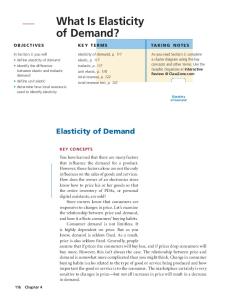
Previously to the estimation of the demand equation, the main variables of the study traffic intensity and toll per kilometre- were examined with the purpose of identifying their evolution through time and the particular characteristics of each section. In the following paragraphs the main facts are highlighted. With respect to traffic intensity, a clear relation with the evolution of GDP is observed, even though it is subject to specific changes occurred in each motorway. Figure 1 shows the synchronism between the rates of growth of GDP and traffic intensity for the whole motorway network. It is also interesting to observe the behaviour of the traffic intensity and the GDP cycles7. As it can be seen in Figure 2, the traffic cycle clearly overreacts to the GDP cycle. Therefore, in periods of economic expansion, the cyclical components of the traffic intensity surpass the corresponding components of the GDP, while the opposite happens during recession. When specific motorway sections are looked at, a significant difference is observed in the traffic intensity among the different motorways as well as among sections of the same motorway. The daily average traffic intensity ranges from 1,689 vehicles per day in the section and year with the lowest intensity to 63,741 vehicles per day in the section and year with the highest one. Finally, it can be pointed out that toll rates are set in such a way that revenue in each motorway has to cover construction and operating costs. This criterion creates an extensive range of prices that vary according to the construction costs and the traffic level in each motorway. This variation permits a more reliable estimation of price elasticity8. For the whole period, at prices of 1992, the lowest price paid per km. was around 0.037 euros whereas the highest was around 0.22 euros. 5. Results The results of the estimated model –equation 5 above- show that all the coefficients have the expected sign and that most of them have been estimated with a high degree of reliability as measured by the t-statistic9. Given that heteroscedasticity was observed in the error term, the model was estimated using Weighted Least Squares. This maintains

10

the estimates’ values while their standard errors decrease. With relation to the toll coefficients a significant variation across motorway sections was observed. A Chisquare test allowed us to clearly reject the null hypothesis of equality of toll coefficients across all sections10. On the other hand, from the analysis of the toll coefficients –which given the model specification correspond to the short term elasticity- it was apparent that they follow certain patterns. First, adjacent sections in the same motorway present very similar elasticities; second, the more inelastic sections are located on corridors with a high traffic density -mainly the motorways along the Mediterranean coast- and thirdly, demand show to be more elastic where a good road alternative exists. For instance, the toll elasticity in the sections of a same motorway -in absolute value- is directly related to the quality of the alternative road. The observed results suggested the possibility of grouping the motorway sections according to their estimated values for the toll elasticities. The model was reestimated introducing cross-equation constraints and classifying the motorway sections into the following groups: 1- Low short term elasticity. Between 0 and -0.3. 2- Middle-low short term elasticity. Between -0.3 and -0.4. 3- Middle-high short term elasticity. Between -0.4 and -0.6. 4- High short term elasticity. Larger than -0.6 in absolute value. Thus, four different coefficients for toll elasticities are now estimated. The detailed results of this final model are presented in Table A.1 of the appendix D and correspond to the estimation by Weighted Least Squares. The application of a Chi-square test did not reject the hypothesis of grouping the motorway sections into four groups according to their estimated toll elasticity11. The estimation of a demand equation from a panel of observations that covers a wide spectrum of motorways and, as a consequence, provides a large degree of variability in the sample, has proved that the traffic on tolled motorways is clearly sensitive to the variables considered a priori. Again, the high degree of reliability of all estimated

11

coefficients should be stressed. This is a sound support for the conclusions derived from the analysis. With respect to the toll coefficients, significant differences among them can be observed, according to the grouping by sections mentioned above. All the dummy variables take the expected sign; it should be noted that the inclusion of these variables increased the statistical significance of toll variable estimates without modifying their value in any way. Table 3 summarises the estimated elasticities. Traffic on tolled motorways is very sensitive to the evolution of economic activity and the figures showed in table 3 are fully in agreement with the visual impression that figures 1 and 2, previously described, provide. Demand elasticity with respect to GDP is estimated to be 0.89 in the short term and 1.41 in the long term. The elasticity with respect to petrol price equals –0.34 in the short run and –0.53 in long run. Our results are consistent with those reported in the literature12 although they are closer to the maximum reported values. This higher sensitivity of tolled motorway users, compared to other estimations carried out for freeways, can be explained by the fact that the former has the untolled roads as an alternative. Besides, the results also clearly show that individuals react to toll variations. Given the high precision with which the elasticities have been estimated this study brings evidence against the rigidity of the demand with regard to the motorway price. However, there is a clear difference among groups of motorways. For the first group that has been defined, the elasticity takes quite low values. However, for the rest of the groups, the elasticity increases and for the fourth one it reaches really high values with a short-term elasticity close to -0.8 and a long-term value above unity. These differences point out the importance of the characteristics of the transport supply when measuring the response of the individuals to the toll variations. In relation to the dynamic structure of traffic demand, the long-term price and income effects are about 50 per cent higher than in the short term, reflecting a wider range of opportunities and available options open to individuals in a longer time span. However, the period of adjustment is relatively short, with the changes being practically completed in a couple of years.

12

In order to explain the variability across the low, middle-low, middle-high and high categories of toll elasticities an ordered probit model has been estimated. The dependent variable is the category where the tolled section falls, ranging from 1 to 4. The set of the explanatory variables is composed of the following. Two variables that capture the quality of the alternative road: average speed and percentage of heavy vehicles with respect to total traffic; length of the section and a dummy variable that equals 1 when tourist traffic represents a significant share of total traffic in the motorway section. The underlying idea is that, as the alternative route becomes less attractive, the price elasticity of the demand becomes more rigid. Let us consider the speed of the alternative route as an example. As the speed of the free route is reduced, the cost in terms of time for not using the motorway will increase and therefore the price elasticity will decrease. However, to the extent that price elasticity is estimated as a discrete variable that can be located in four categories, an ordered probit, or logit, model is the standard way to deal with the problem. In fact, from an economic point of view it is irrelevant which of the two models is selected. We have used as a first option the probit approach because the normality hypothesis has a long econometric tradition13. The total number of observations was reduced from 72 to 52, as we could not collect all the required information for 20 sections. Table 4 shows the main estimation results while the full model is presented in table A.2 of the appendix D. The estimation shows that demand is more sensitive to price when the free alternative road has a better quality. That is, the higher the speed on the alternative road and the lower the percentage of heavy vehicles, the more elastic demand is. Besides, elasticities seem to depend on the length of the section and on the presence of tourist traffic on the motorways. That is, foreign visitors, due to lack of information, could be less sensitive to price than other motorway users. 6. Conclusions The estimation of a demand function on tolled motorways allows us to identify the behavioural responses of their users to changes in the explanatory variables. First of all,

13

traffic on the tolled motorways is shown to be strongly correlated with the economic activity level in such a way that during expansions traffic growth clearly exceeds GDP growth and the opposite occurs during recessions. Travel demand is also shown to be sensitive to monetary costs. The elasticity with respect to petrol price is around -0.3, whereas significant differences appear in toll elasticities across motorway sections. The model results prove that a unique aggregate elasticity cannot be considered as a valid one in order to evaluate behavioural responses to toll changes. According to the individual estimations, the sections have been grouped in four categories for which the short-term elasticity ranges from -0.21 on the most inelastic sections to -0.83 on the most elastic ones. This range of variation can be best explained by those variables related to the quality of the alternative roads, the length of the motorway section and the presence of tourist traffic. The more congested the alternative roads are, the higher the time benefits of using the tolled motorway will be, and so the more rigid is the demand. The findings of this study show that there might be a wide range of policy opportunities to influence the pattern of travel demand. On the one hand, pricing will have important consequences in terms of traffic allocation between roads, with its cumulative effects increasing over time. In those cases where tolls are exclusively used to raise revenue in order to finance motorway construction and maintenance, pricing the motorway will shift demand from the tolled to the untolled alternative. The tolled motorway will be under-used whereas traffic will shift to the free alternative with the consequent increase in maintenance, congestion and environmental costs. Given that demand elasticities in the tolled road can be rather high in some specific contexts, the costs of traffic distortions will be significant, so will be the possible negative impact on welfare. Verhoef et al. (1996) show the crucial importance of demand elasticities when evaluating the efficiency of one-route tolling. Besides, it should be noted that the effects take place at network level -for example, a toll reduction may increase the congestion in the roads feeding the motorway and therefore this should be taken into account when evaluating changes in toll rates.

14

Moreover, investment on alternative transport roads or modes will imply a more elastic demand for motorway users, as they will face a wider range of behavioural possibilities. Therefore, the decisions about the toll level on the motorways are not independent from the investment policy in transport infrastructure. For the same reason the social benefits derived from the toll motorway construction are lower when there is a good alternative. Nevertheless, such findings should be treated with caution given that we have only taken into account some of the factors that affect the variability of toll elasticity. Motorist’s response to changes in price depends on multiple circumstances among which an important one should be pointed at: Individuals’ preferences are not usually as similar as it is assumed in an aggregate demand equation, and in particular they depend on their value of time. If heterogenity in value of time were accounted for in estimating the demand model, we would find a range of elasticities values instead of an average value. But at aggregate level, and given the available information, only average values can be obtained, and it is in this way that our estimates must be interpreted. Acknowledgments This study has had the inestimable co-operation of Alvaro Angeriz as a research assistant. We also must thank Javier Asensio and three anonymous referees for their helpful suggestions and comments. We are also grateful to Mark Burris for providing some references about toll elasticities in the US. Financial support for this study was provided by the Spanish Ministerio de Fomento and the CICYT programme (project SEC97-1333). The authors gratefully acknowledge the support received from the Ministerio de Fomento, from the Asociación de Sociedades Españolas Concesionarias de Autopistas and from the concessionary companies.

Notes 1

This assumption was made after an analysis of the transport supply in Spain. Those motorway sections for which the previous hypothesis did not hold were excluded from the sample. However, this only affected a very small number of sections, mainly those located around urban areas. 2 The recursive least squares technique consists of estimating the model adding new temporal observations in a progressive way, which makes it possible to test the stability of the coefficient vector. If the coefficient displays significant variation as more data is added to the estimating equation, it is a strong indication of instability. 3 For a standard reference about unit root and cointegration tests see Hamilton (1994). All the results of the applied test are available from request. 4 The Johansen test was not applied to test cointegration because this test assumes the existence of a feedback between all the variables. In our case, variables like petrol price, toll and GDP must be considered as weakly exogenous in a model that tries to explain the motorway traffic intensity. 5 Given that the equation is estimated in first differences of the logarithms and that it includes the lagged dependent variable, the final number of observations is reduced to 990.

15

6

It has to be noted that the dependent variable is an aggregate of different types of traffics of different length and purpose. Therefore, the estimated elasticity for each section has to be understood as an average value. 7 The cycles of both variables were obtained through the application of the Hodrick-Prescot filter to the log of the series and calculating the difference between the observed values and the trend values. 8 The way in which tolls are fixed in the opening year could create an endogeneity problem as long as in more intensively travelled road sections the toll is lower. Nonetheless, this problem does not arise in our estimation given that the variables are expressed in first difference of the logarithm and the criteria used to allow for price changes is not related in any way to changes in traffic volume. We must thank an anonymous referee for this comment. 9 The output of this estimation is not reported here because, given the high number of estimated coefficients, it would be too cumbersome and it does not add anything to the final results. Nonetheless, it is available from the authors on request. 10 The calculated Chi-square statistic was 113.12, while the tabulated value for 71 degrees of freedom (d.f) at a significance level of 5 per cent is 52.0. 11 The calculated Chi-square statistic was 13.27, while the tabulated value for 68 d.f. at a significance level of 5 per cent is 49.0. 12 For a literature review of such findings see Goodwin (1992), Oum et al. (1992), Johannson and Shipper (1997), Espey (1998) and de Jong (2001). 13 When an ordered logit model was used, the following results were obtained: Variable Coefficient t-statistic Speed in the alternative road 0.0558 3.064 Heavy vehicles on the alternative road -0.0855 -2.936 Motorway section length 0.0395 2.230 Tourist dummy -2.134 -3.326 However, as is well known, the estimated coefficients of the logit and probit model are not directly comparable. The usual way to compare both formulations is in terms of calculating the marginal response of the probability facing an increase of the explanatory variables, evaluating such probabilities taking 0.5 as starting point. To achieve this, the logit coefficients must be multiplied by 0.25, and the probit coefficients by 0.40. After this transformation, the marginal effects of each explanatory variable in both formulations, are the following: Marginal effects in both formulations Variable Probit Logit Speed in the alternative road 0.01277 0.01395 Heavy vehicles on the alternative road 0.02106 0.02138 Motorway section length 0.00962 0.00987 Tourist dummy -0.49102 -0.53355

16

Appendix A In Spain, the toll motorway construction policy started in the sixties by granting concessions to private companies for both their construction and operation. As a result of such policy 1,800 kilometres of tolled motorways, called “autopistas”, were in service by the end of the seventies, which served demand along two main traffic corridors. Once the main traffic corridors had been concessioned and, simultaneously, the Spanish economy was suffering the effects of the energy crisis, private capital was no longer interested in the construction of “autopistas”. Since the mid seventies the concession of the planned motorways was increasingly difficult, some of them were postponed and finally the whole policy was abandoned at the end of the decade. In the eighties the need for a significant expansion of the road network was evident and the government’s decision was to finance it through national tax revenue and approximately some 5,500 kilometres of untolled motorways were constructed until 1998 which mostly fill in the national network. The main exceptions were the concessions granted by the regional government of Catalonia to construct and operate some tolled motorways. By 1998 the Spanish national highway network consisted of 9,637 kilometres of which 2,072 correspond to tolled motorways, 6,185 to untolled motorways and 1,380 to double lane freeways. In the last years, and due to severe public budget constraints, a new programme of private tolled motorways is in progress; nevertheless the scope for private tolled roads in Spain is nowadays limited. Appendix B In order to compare the goodness of fit of the linear and the log-linear functional forms, a way to proceed is to compare the sum of squares of residuals (SSR) of both models after establishing an appropriate correction. That is, the residuals of the linear model have to be divided by the value of the dependent variable in order to obtain a residual sum of squares that can be properly compared with that of the log linear model. In the case we have equations Y = X´α + u and lnY = (lnX´)β + e, in order to compare homogeneous magnitudes, the SSR of ê must be compared with the SSR of û/Y, because ) in the log-linear model ê directly approximates the difference (Y − Y ) / Y . Box and Cox (1962) suggest a more formal criterion based on the likelihood function. In this case, the log of the likelihood function of the linear model can be compared with the log of the likelihood function of the log-linear model, but refereeing both log likelihood to the levels of the dependent variable. As it is well known, under standard hypothesis, the log of the likelihood function of the linear model is given by: ln (Likelihood linear model) = Const.- (T/2)·ln(SSR linear model/T), where T is the sample size and SSR the residual sum of squares. In the case that the Data Generating Process corresponds to the log-linear model, the log-likelihood function referred to the levels of the dependent variable could be expressed as: T ln(Likelihood log-linear model) = Const.-(T/2)·ln(SSR log-linearmodel)- ∑1 ln(Y), where Y is the dependent variable.

17

The problem of selecting the more adequate functional form is solved comparing the values that both log-likelihood functions reach.

Appendix C Definition of the dummy variables included in the estimated demand equation. These variables take the value 1 in the reported period and 0 otherwise. Dummy variables D(1) to D(4)

Period

Comment

1994-1998

They reflect the negative impact on the traffic of the four sections of motorway A(2) derived from the capacity and quality improvements on the alternative free road. D(5) to D(7) 1992 They account for the positive impact on the three sections of motorway A(4) derived from the Sevilla World Exhibition in 1992. D(8) to D(11) 1995-1998 They reflect the negative impact on the traffic of four sections of motorway A(7) as a consequence of the enlargement of an alternative tollway. D(12), D(14) and 1993-1998 They reflect the negative impact on the traffic of three sections of D(16) motorway A(7) derived from the opening of an alternative free motorway. D(13), D(15) and 1990-1998 They account for the positive impact on the traffic of ten sections of D(17) to D(24) motorway A(7) due to an enlargement of this motorway. D(25) 1996-1998 It reflects changes in the motorway network around the first section of motorway A(19). D(26), D(27) and 1994-1998 They account for the positive impact on the traffic of the three sections D(28) of motorway A(66) as a consequence of the improvement and enlargement of the motorway. Note: In Spain the motorways (autopistas) are named with an A followed of a number in brackets.

18

Appendix D Table A.1. Table A.2.

References Box GEP & Cox DR (1962) An analysis of transformations. Journal of the Royal Statistical Society, Series B: 211-243. Burris MW, Cain A & Pendyala RM (2001) Impact of variable pricing on temporal distribution of travel demand. Transportation Research Record, 1747: 36-43. Gifford JL & Talkington SW (1996) Demand elasticity under time-varying prices: case study of day-of-week varying tolls on Golden Gate Bridge. Transportation Research Record, 1558: 55-59. Hamilton JD (1994) Time series analysis, Princeton University Press, New Jersey Harvey G (1994) Transportation pricing behavior. In Curbing Gridlock: Peak-Period Fees to Relieve Traffic Congestion, 2 (pp 89-114). Transportation Research Board, Special Report 242, National Academy Press. Hirschman I, McNight C, Pucher J, Paaswell RE & Berechman J (1995) Bridge and tunnel toll elasticities in New York. Some recent evidence. Transportation, 22: 97113. Jones P & Hervik A (1992) Restraining car traffic in European cities: an emerging role for road pricing. Transportation Research-A, 26: 133-145. Mauchan A & Bonsall P (1995) Model predictions of the effects of motorway charging in West Yorkshire. Traffic, Engineering and Control, 36: 206-212. May AD (1992) Road pricing: an international perspective. Transportation, 19: 313333. Ministerio de Fomento Memoria. Delegación del Gobierno en las Sociedades Concesionarias de Autopistas de Peaje, Secretaria de Estado de Infraestructuras y Transportes, Ministerio de Fomento, Madrid. Ministerio de Fomento El tráfico en las autopistas de peaje. Dirección General de Carreteras, Ministerio de Fomento, Madrid.

19

Oum TH, Waters WG & Yong JS (1992) Concepts of price elasticities of transport demand and recent empirical estimates. Journal of Transport Economics and Policy, 26: 139-154. Ribas E, Raymond JL & Matas A (1988) Estudi sobre la elasticitat preu de la demanda de tràfic per autopista. Departament de Política Territorial i Obres Públiques, Generalitat de Catalunya, Barcelona. TRACE Consortium (1998) Deliverable 1: Outcomes of Review on Elasticities and Values of Time. TRACE Consortium, The Hague. UTM (2000) Traffic responses to toll increases remains inelastic. The Urban Transport Monitor, 14 (10), Lawley Publications. Verhoef E, Nijkamp P & Rietveld P (1996) Second-Best Congestion Pricing: The Case of an Untolled Alternative. Journal of Urban Economics, 40: 279-302. Weustefield NH & Regan EJ (1981) Impact of rate increases on toll facilities. Traffic Quarterly, 34: 639-55.

20

Table 1. Elasticity of traffic level with respect to toll. Authors Results Weustefield and Regan (1981)

Context

Roads between -0.03 and –0.31 Bridges between -0.15 and –0.31 Average value -0.21 White (1984), quoted in Oum et Peak hours between -0.21 and -0.36 al. (1992) Off-peak hours between -0.14 and 0.29 Goodwin (1988), quoted in May Average value -0.45 (1992)

Sixteen tolled infrastructures in the US (roads, bridges and tunnels) Bridge in Southampton.UK.

Ribas, Raymond and Matas Between -0.15 and -0.48 (1988)

Three intercity motorways in Spain

Jones and Hervik (1992)

Toll ring schemes. Norway.

Harvey (1994)

Oslo –0.22 Alesund -0.45 Bridges between –0.05 and –0.15 Roads –0.10

Literature review of a number of previous studies

Golden Gate Bridge, San Francisco Bay Bridge and Everett Turnpike in New Hampshire. US. Hirschman, McNight, Pucher, Between –0.09 and -0.50 Six bridges and two tunnels in Paaswell and Berechman (1995) Average value -0.25 (only significant New York City area. US. values quoted) Mauchan and Bonsall (1995)

Whole motorway network -0.40 Intercity motorways -0.25

Simulation model of motorway charging in West Yorkshire. UK Gifford and Talkington (1996) Own-elasticity of Friday-Saturday Golden Gate Bridge, San traffic –0.18 Francisco. US. Cross-elasticity of Monday-Thursday traffic with respect to Friday toll -0.09 INRETS (1997), quoted in Between –0.22 and –0.35 French motorways for trips TRACE (1998) longer than 100 kilometres UTM (2000) -0.20 New Jersey Turnpike. US. Burris, Cain and Pendyala Off-peak period elasticity with respect Lee County, Florida. US. (2001) to off-peak toll discount between –0.03 and –0.36

21

Table 2. Descriptive statistics. Variables

Average

Maximum

Minimum

Std. Dev.

Observations

11,490

63,741

1,689

8,821

1135

0.091

0.224

0.037

0.035

1135

0.619

0.867

0.486

0.139

19

219,311

275,869

174,149

33,619

19

14.7

43.0

2.0

8.2

72

Daily traffic intensity Toll (euros per km.)

1 1

Petrol price (euros per litre) 1

GDP (millions of euros) Section length (kms) 1

The base year for those variables expressed in monetary units is 1992.

Table 3. Estimated elasticities on short and long term by groups of motorways1. VARIABLE

SHORT TERM tLONG TERM tELASTICITY statistic ELASTICITY statistic GDP-elasticity 0.890 21.76 1.405 27.85 Petrol price elasticity -0.336 -22.01 -0.531 -18.50 Toll elasticity group 1 -0.209 -11.77 -0.330 -11.42 Toll elasticity group 2 -0.371 -25.21 -0.585 -21.71 Toll elasticity group 3 -0.445 -19.80 -0.702 -17.66 Toll elasticity group 4 -0.828 -9.80 -1.307 -9.81 1 Groupe 1 includes 21 sections; group 2, 25 sections; group 3, 21 sections and group 4, 5 sections.

Table 4: Main results of the estimated ordered probit model. Dependent variable: Category of toll elasticity (from 1 to 4) Variable

Coefficient

t-statistic

Speed in the alternative road

0.032

3.121

Heavy vehicles on the alternative road

-0.053

-3.042

Motorway section length

0.024

2.516

Tourist dummy

-1.227

-3.433

22

Figure 1. Rate of growth of GDP and traffic intensity 0.06 0.04 0.15 0.02

0.10 0.05

0.00

0.00

-0.02

-0.05 -0.10 80

82

84

86

88

90

D(LTRAFFIC), left scale

92

94

96

D(LGDP), right scale

Figure 2. GDP cycle and traffic cycle 0.15 0.10 0.05 0.00 -0.05 -0.10 -0.15 80

82

84

GDP cycle

86

88

90

92

94

96

TRAFFIC cycle

23

Table A.1. Estimated demand equation Dependent variable: D(LTRAFFIC) Estimation Method: Weighted Least Squares Total system (unbalanced) observations 990 Sample: 1981 1998 Number of cross-sections used: 72 Variable

Coefficient

Std. Error

t-Statistic

Prob.

D(LGDP) 0.890193 D(LPETROL) -0.336743 D(LTRAFFIC(-1)) 0.365883 D(LTOLL1) -0.209230 D(LTOLL2) -0.370693 D(LTOLL3) -0.444932 D(LTOLL4) -0.828583 D(1) -0.051684 D(2) -0.068902 D(3) -0.071780 D(4) -0.051897 D(5) 0.154926 D(6) 0.168991 D(7) 0.119571 D(8) -0.067818 D(9) -0.062270 D(10) -0.065594 D(11) -0.042454 D(12) -0.054993 D(13) 0.074554 D(14) -0.033741 D(15) 0.062609 D(16) -0.035954 D(17) 0.049779 D(18) 0.044454 D(19) 0.040371 D(20) 0.052885 D(21) 0.169750 D(22) 0.081240 D(23) 0.082155 D(24) 0.137853 D(25) -0.136566 D(26) 0.086360 D(27) 0.075056 D(28) 0.045058 0.74 R2 (average for the motorway sections) First order autocorrelation coefficient 0.019 (average for the motorway sections)

0.040909 0.015303 0.015807 0.017712 0.014682 0.022471 0.084395 0.025947 0.023940 0.024600 0.026283 0.039587 0.036369 0.058307 0.021852 0.020069 0.028630 0.022716 0.024980 0.025104 0.020086 0.020228 0.018751 0.018879 0.019199 0.015294 0.013367 0.043344 0.016342 0.020701 0.018653 0.048787 0.017716 0.017495 0.020577

21.76049 -22.00499 23.14699 -11.81297 -25.24832 -19.80068 -9.817902 -1.991921 -2.878151 -2.917925 -1.974532 3.913600 4.646551 2.050702 -3.103508 -3.102872 -2.291089 -1.868884 -2.201487 2.969813 -1.679843 3.095231 -1.917461 2.636744 2.315442 2.639679 3.956290 3.916315 4.971190 3.968585 7.390278 -2.799232 4.874603 4.290238 2.189731

0.0000 0.0000 0.0000 0.0000 0.0000 0.0000 0.0000 0.0467 0.0041 0.0036 0.0486 0.0001 0.0000 0.0406 0.0020 0.0020 0.0222 0.0619 0.0279 0.0031 0.0933 0.0020 0.0555 0.0085 0.0208 0.0084 0.0001 0.0001 0.0000 0.0001 0.0000 0.0052 0.0000 0.0000 0.0288

Note: All the variables are defined in first differences of the logarithm. GDP: Gross Domestic Product; PETROL: petrol price; TRAFFIC: average traffic intensity, TOLL1: toll low elasticity group; TOLL2: toll low-medium elasticity group, TOLL3: toll medium-high elasticity group; TOLL4: toll high elasticity group; D(1) to D(28): dummy variables to account for changes in the road network.

24

Table A.2. Explanatory ordered probit model of toll elasticities differences across groups of motorways Dependent variable: Category of toll elasticity (from 1 to 4) Variable Coefficient Std. Error t-statistic Speed in the alternative road 0.032 0.0102 3.1212 Percentage of heavy vehicles on the alternative road -0.053 0.0173 -3.0419 Motorway section length 0.024 0.0096 2.5160 Tourist dummy -1.227 0.3576 -3.433 Limit_1 0.919 0.8624 1.066 Limit_2 2.393 0.9202 2.601 Limit_3 3.666 0.9622 3.810 Observations 52 Likelihood ratio-statistic 25.60 (critical value at 5 %: 9.49)

Prob. 0.0018 0.0024 0.0119 0.0006 0.2865 0.0093 0.0001

25