The Stokes Theorem. (Sect. 16.7)
I
The curl of a vector field in space.
I
The curl of conservative fields.
I
Stokes’ Theorem in space.
I
Idea of the proof of Stokes’ Theorem.
The curl of a vector field in space. Definition The curl of a vector field F = hF1 , F2 , F3 i in R3 is the vector field
� curl F = (∂2 F3 − ∂3 F2 ), (∂3 F1 − ∂1 F3 ), (∂1 F2 − ∂2 F1 ) .
Remark: Since the following formula holds, i j k curl F = ∂1 ∂2 ∂3 F 1 F 2 F 3 curl F = (∂2 F3 − ∂3 F2 ) i − (∂1 F3 − ∂3 F1 ) j + (∂1 F2 − ∂2 F1 ) k, then one also uses the notation curl F = ∇ × F.
The curl of a vector field in space. Example Find the curl of the vector field F = hxz, xyz, −y 2 i. Solution: Since curl F = ∇ × F, we get, i j k ∂z = ∇ × F = ∂x ∂y xz xyz −y 2 � � � ∂y (−y 2 )−∂z (xyz) i− ∂x (−y 2 )−∂z (xz) j + ∂x (xyz)−∂y (xz) k, � � � = −2y − xy i − 0 − x j + yz − 0 k, We conclude that ∇ × F = h−y (2 + x), x, yzi.
The Stokes Theorem. (Sect. 16.7)
I
The curl of a vector field in space.
I
The curl of conservative fields.
I
Stokes’ Theorem in space.
I
Idea of the proof of Stokes’ Theorem.
C
The curl of conservative fields. Recall: A vector field F : R3 → R3 is conservative iff there exists a scalar field f : R3 → R such that F = ∇f .
Theorem If a vector field F is conservative, then ∇ × F = 0.
Remark: I
This Theorem is usually written as ∇ × (∇f ) = 0.
I
The converse is true only on simple connected sets. That is, if a vector field F satisfies ∇ × F = 0 on a simple connected domain D, then there exists a scalar field f : D ⊂ R3 → R such that F = ∇f .
Proof of the Theorem: ∇×F =
� � �� ∂y ∂z f − ∂z ∂y f , − ∂x ∂z f − ∂z ∂x f , ∂x ∂y f − ∂y ∂x f
The curl of conservative fields. Example Is the vector field F = hxz, xyz, −y 2 i conservative? Solution: We have shown that ∇ × F = h−y (2 + x), x, yzi. Since ∇ × F 6= 0, then F is not conservative.
C
Example Is the vector field F = hy 2 z 3 , 2xyz 3 , 3xy 2 z 2 i conservative in R3 ? Solution: Notice that i j k ∂y ∂z ∇ × F = ∂x y 2 z 3 2xyz 3 3xy 2 z 2
� = (6xyz 2 − 6xyz 2 ), −(3y 2 z 2 − 3y 2 z 2 ), (2yz 3 − 2yz 3 ) = 0. Since ∇ × F = 0 and R3 is simple connected, then F is conservative, that is, there exists f in R3 such that F = ∇f .
C
The Stokes Theorem. (Sect. 16.7)
I
The curl of a vector field in space.
I
The curl of conservative fields.
I
Stokes’ Theorem in space.
I
Idea of the proof of Stokes’ Theorem.
Stokes’ Theorem in space. Theorem The circulation of a differentiable vector field F : D ⊂ R3 → R3 around the boundary C of the oriented surface S ⊂ D satisfies the equation I ZZ F · dr = C
(∇ × F) · n dσ, S
where dr points counterclockwise when the unit vector n normal to S points in the direction to the viewer (right-hand rule). n S
C r’ (t)
r (t)
Stokes’ Theorem in space. Example Verify Stokes’ Theorem for the field F = hx 2 , 2x, z 2 i on the ellipse S = {(x, y , z) : 4x 2 + y 2 6 4, z = 0}. I ZZ Solution: We compute both sides in F · dr = (∇ × F) · n dσ. C
We start computing the circulation 2 integral on the ellipse x 2 + y22 = 1. We need to choose a counterclockwise parametrization, hence the normal to S points upwards. We choose, for t ∈ [0, 2π],
z
−1
S
−2
2
C
S
y
1
x
z n −1
−2
r(t) = hcos(t), 2 sin(t), 0i.
S
2
C
y
Therefore, the right-hand rule normal n to S is n = h0, 0, 1i.
1
x
Stokes’ Theorem in space. Example Verify Stokes’ Theorem for the field F = hx 2 , 2x, z 2 i on the ellipse S = {(x, y , z) : 4x 2 + y 2 6 4, z = 0}. I ZZ Solution: Recall: F · dr = (∇ × F) · n dσ, with C
S
r(t) = hcos(t), 2 sin(t), 0i, t ∈ [0, 2π] and n = h0, 0, 1i. The circulation integral is: I Z 2π F(t) · r0 (t) dt F · dr = 0
C
Z =
2π
hcos2 (t), 2 cos(t), 0i · h− sin(t), 2 cos(t), 0i dt.
0
I
Z F · dr =
C
0
2π �
� − cos2 (t) sin(t) + 4 cos2 (t) dt.
Stokes’ Theorem in space. Example Verify Stokes’ Theorem for the field F = hx 2 , 2x, z 2 i on the ellipse S = {(x, y , z) : 4x 2 + y 2 6 4, z = 0}. I Z 2π � � Solution: F · dr = − cos2 (t) sin(t) + 4 cos2 (t) dt. 0
C
The substitution on the first term u = cos(t) and du = − sin(t) dt, Z 2π Z 1 2 − cos (t) sin(t) dt = u 2 du = 0. implies 0
1
I
Z
2π
Z
2
F · dr =
2π
� � 2 1 + cos(2t) dt.
4 cos (t) dt = 0
C
0
2π
Z Since
I F · dr = 4π.
cos(2t) dt = 0, we conclude that 0
C
Stokes’ Theorem in space. Example Verify Stokes’ Theorem for the field F = hx 2 , 2x, z 2 i on the ellipse S = {(x, y , z) : 4x 2 + y 2 6 4, z = 0}. I Solution: F · dr = 4π and n = h0, 0, 1i. C
We now compute the right-hand side in Stokes’ Theorem. z
ZZ
n −1
(∇ × F) · n dσ.
I =
S
S
−2
2
C
y
1
x
i j ∇ × F = ∂x ∂y x 2 2x S is the flat surface {x 2 +
k ∂z z 2 y2 22
⇒
∇ × F = h0, 0, 2i.
6 1, z = 0}, so dσ = dx dy .
Stokes’ Theorem in space. Example Verify Stokes’ Theorem for the field F = hx 2 , 2x, z 2 i on the ellipse S = {(x, y , z) : 4x 2 + y 2 6 4, z = 0}. I Solution: F · dr = 4π, n = h0, 0, 1i, ∇ × F = h0, 0, 2i, and C
dσ = dx dy . ZZ Z Then, (∇ × F) · n dσ =
1
−1
S
Z
√ 2 1−x 2
h0, 0, 2i √ −2 1−x 2
· h0, 0, 1i dy dx.
The right-hand side above is twice the area of the ellipse. Since we know that an ellipse x 2 /a2 + y 2 /b 2 = 1 has area πab, we obtain ZZ (∇ × F) · n dσ = 4π. S
This verifies Stokes’ Theorem.
C
Stokes’ Theorem in space. Remark: Stokes’ Theorem implies that for any smooth field F and any two surfaces S1 , S2 having the same boundary curve C holds, ZZ ZZ (∇ × F) · n1 dσ1 = (∇ × F) · n2 dσ2 . S1
S2
Example Verify Stokes’ Theorem for the field F = hx 2 , 2x, z 2 i on any y2 z2 2 half-ellipsoid S2 = {(x, y , z) : x + 2 + 2 = 1, z > 0}. 2 a Solution: (The previous example was the case a → 0.) We must verify Stokes’ Theorem on S2 , I ZZ F · dr = (∇ × F) · n2 dσ2 .
z n2
n2
a
S2
2
C 1
x
S1
y
C
S2
Stokes’ Theorem in space. Example Verify Stokes’ Theorem for the field F = hx 2 , 2x, z 2 i on any y2 z2 half-ellipsoid S2 = {(x, y , z) : x 2 + 2 + 2 = 1, z > 0}. 2 a I
ZZ
Solution:
F · dr = 4π, ∇ × F = h0, 0, 2i, I = C
(∇ × F) · n2 dσ2 . S2
z
S2 is the level surface F = 0 of
n2
n2
a
S2
2
C 1
y2 z2 F(x, y , z) = x + 2 + 2 − 1. 2 a 2
y
S1
x
∇F n2 = , |∇F|
|∇F| |∇F| = 2z/a2 |∇F · k|
dσ2 =
2z/a2 (∇ × F) · n2 = 2 . |∇F|
y 2z E ∇F = 2x, , 2 , 2 a D
⇒
(∇ × F) · n2 dσ2 = 2.
Stokes’ Theorem in space. Example Verify Stokes’ Theorem for the field F = hx 2 , 2x, z 2 i on any y2 z2 2 half-ellipsoid S2 = {(x, y , z) : x + 2 + 2 = 1, z > 0}. 2 a I F · dr = 4π and (∇ × F) · n2 dσ2 = 2. Solution: C
Therefore, ZZ
ZZ (∇ × F) · n2 dσ2 =
2 dx dy = 2(2π). S1
S2
ZZ (∇ × F) · n2 dσ2 = 4π, no matter what is
We conclude that the value of a > 0.
S2
C
The Stokes Theorem. (Sect. 16.7)
I
The curl of a vector field in space.
I
The curl of conservative fields.
I
Stokes’ Theorem in space.
I
Idea of the proof of Stokes’ Theorem.
Idea of the proof of Stokes’ Theorem. S
Split the surface S into n surfaces Si , for i = 1, · · · , n, as it is done in the figure for n = 9. C
I F · dr = C
n I X
F · dri
Ci
' =
i=1 n I X
F · d˜ri
˜ i=1 C i n ZZ X
Zi=1 Z
˜i the border of small rectangles); (C
(∇ × F) · ni dA (Green’s Theorem on a plane);
˜i R
(∇ × F) · n dσ.
' S
The Divergence Theorem. (Sect. 16.8)
I
The divergence of a vector field in space.
I
The Divergence Theorem in space.
I
The meaning of Curls and Divergences. Applications in electromagnetism:
I
I I
Gauss’ law. (Divergence Theorem.) Faraday’s law. (Stokes Theorem.)
The divergence of a vector field in space. Definition The divergence of a vector field F = hFx , Fy , Fz i is the scalar field div F = ∂x Fx + ∂y Fy + ∂z Fz .
Remarks: I
It is also used the notation div F = ∇ · F.
I
The divergence of a vector field measures the expansion (positive divergence) or contraction (negative divergence) of the vector field.
I
A heated gas expands, so the divergence of its velocity field is positive.
I
A cooled gas contracts, so the divergence of its velocity field is negative.
The divergence of a vector field in space. Example Find the divergence and the curl of F = h2xyz, −xy , −z 2 i. Solution: Recall: div F = ∂x Fx + ∂y Fy + ∂z Fz . ∂x Fx = 2yz,
∂y Fy = −x,
∂z Fz = −2z.
Therefore ∇ · F = 2yz − x − 2z, that is ∇ · F = 2z(y − 1) − x. Recall: curl F = ∇ × F. i j k ∂y ∂z = h(0 − 0), −(0 − 2xy ), (−y − 2xz)i ∇ × F = ∂x 2xyz −xy −z 2 We conclude: ∇ × F = h0, 2xy , −(2xz + y )i.
C
The divergence of a vector field in space. Example
r Find the divergence of F = 3 , where r = hx, y , zi, and ρ p ρ = |r| = x 2 + y 2 + z 2 . (Notice: |F| = 1/ρ2 .) y z x F = , F = . , y z ρ3 ρ3 ρ3 � �−3/2 � ∂x Fx = ∂x x x 2 + y 2 + z 2
Solution: The field components are Fx =
∂x Fx = x 2 + y 2 + z 2
�−3/2
�−5/2 3 − x x2 + y2 + z2 (2x) 2
1 y2 1 x2 ∂x Fx = 3 − 3 5 ⇒ ∂y Fy = 3 − 3 5 , ρ ρ ρ ρ
1 z2 ∂z Fz = 3 − 3 5 . ρ ρ
3 (x 2 + y 2 + z 2 ) 3 ρ2 3 3 ∇·F= 3 −3 = − 3 = − . ρ ρ5 ρ3 ρ5 ρ 3 ρ3 We conclude: ∇ · F = 0.
C
The Divergence Theorem. (Sect. 16.8)
I
The divergence of a vector field in space.
I
The Divergence Theorem in space.
I
The meaning of Curls and Divergences. Applications in electromagnetism:
I
I I
Gauss’ law. (Divergence Theorem.) Faraday’s law. (Stokes Theorem.)
The Divergence Theorem in space. Theorem The flux of a differentiable vector field F : R3 → R3 across a closed oriented surface S ⊂ R3 in the direction of the surface outward unit normal vector n satisfies the equation ZZ ZZZ F · n dσ = (∇ · F) dV , S
V
where V ⊂ R3 is the region enclosed by the surface S.
Remarks: I
The volume integral of the divergence of a field F in a volume V in space equals the outward flux (normal flow) of F across the boundary S of V .
I
The expansion part of the field F in V minus the contraction part of the field F in V equals the net normal flow of F across S out of the region V .
The Divergence Theorem in space. Example Verify the Divergence Theorem for the field F = hx, y , zi over the sphere x 2 + y 2 + z 2 = R 2 . ZZ ZZZ F · n dσ = (∇ · F) dV . Solution: Recall: S
V
We start with the flux integral across S. The surface S is the level surface f = 0 of the function f (x, y , z) = x 2 + y 2 + z 2 − R 2 . Its outward unit normal vector n is n=
∇f , |∇f |
∇f = h2x, 2y , 2zi,
p |∇f | = 2 x 2 + y 2 + z 2 = 2R,
1 hx, y , zi, where z = z(x, y ). R |∇f | R Since dσ = dx dy , then dσ = dx dy , with z = z(x, y ). |∇f · k| z We conclude that n =
The Divergence Theorem in space. Example Verify the Divergence Theorem for the field F = hx, y , zi over the sphere x 2 + y 2 + z 2 = R 2 . 1 R Solution: Recall: n = hx, y , zi, dσ = dx dy , with z = z(x, y ). R ZZ � z ZZ � 1 F · n dσ = hx, y , zi · hx, y , zi dσ. R S S ZZ ZZ ZZ � 1 2 2 2 F · n dσ = x + y + z dσ = R dσ. R S S S The integral on the sphere S can be written as the sum of the integral on the upper half plus the integral on the lower half, both integrated on the disk R = {x 2 + y 2 6 R 2 , z = 0}, that is, ZZ ZZ R F · n dσ = 2R dx dy . S R z
The Divergence Theorem in space. Example Verify the Divergence Theorem for the field F = hx, y , zi over the sphere x 2 + y 2 + z 2 = R 2 . ZZ ZZ R F · n dσ = 2R dx dy . Solution: z S R Using polar coordinates on {z = 0}, we get ZZ Z 2π Z R R2 √ r dr dθ. F · n dσ = 2 R2 − r 2 S 0 0 The substitution u = R 2 − r 2 implies du = −2r dr , so, ZZ
F · n dσ = 4πR 2
Z
u −1/2
R2
S
ZZ
0
F · n dσ = 2πR 2
S
�
R 2 � 1/2 2u 0
(−du) = 2πR 2 2 ZZ ⇒
Z
R2
u −1/2 du
0
F · n dσ = 4πR 3 .
S
The Divergence Theorem in space. Example Verify the Divergence Theorem for the field F = hx, y , zi over the sphere x 2 + y 2 + z 2 = R 2 . ZZ F · n dσ = 4πR 3 . Solution: S ZZZ We now compute the volume integral ∇ · F dV . The V
divergence of F is ∇ · F = 1 + 1 + 1, that is, ∇ · F = 3. Therefore ZZZ ZZZ �4 � 3 ∇ · F dV = 3 dV = 3 πR 3 V V ZZZ We obtain ∇ · F dV = 4πR 3 . V
We have verified the Divergence Theorem in this case.
C
The Divergence Theorem in space. Example
r across the boundary of the region ρ3 between the spheres of radius R1 > R0 > 0, where r = hx, y , zi, p 2 and ρ = |r| = x + y 2 + z 2 . Find the flux of the field F =
Solution: We use the Divergence Theorem ZZ ZZZ F · n dσ = (∇ · F) dV . S
V
ZZZ Since ∇ · F = 0, then
(∇ · F) dV = 0. Therefore V
ZZ F · n dσ = 0. S
The flux along any surface S vanishes as long as 0 is not included in the region surrounded by S. (F is not differentiable at 0.) C
The Divergence Theorem. (Sect. 16.8)
I
The divergence of a vector field in space.
I
The Divergence Theorem in space.
I
The meaning of Curls and Divergences. Applications in electromagnetism:
I
I I
Gauss’ law. (Divergence Theorem.) Faraday’s law. (Stokes Theorem.)
The meaning of Curls and Divergences. Remarks: The meaning of the Curl and the Divergence of a vector field F is best given through the Stokes and Divergence Theorems. I 1 I ∇ × F = lim F · dr, S →{P } A(S) C
I
where S is a surface containing the point P with boundary given by the loop C and A(S) is the area of that surface. ZZ 1 ∇ · F = lim F · ndσ, R →{P } V (R) S where R is a region in space containing the point P with boundary given by the closed orientable surface S and V (R) is the volume of that region.
The Divergence Theorem. (Sect. 16.8)
I
The divergence of a vector field in space.
I
The Divergence Theorem in space.
I
The meaning of Curls and Divergences. Applications in electromagnetism:
I
I I
Gauss’ law. (Divergence Theorem.) Faraday’s law. (Stokes Theorem.)
Applications in electromagnetism: Gauss’ Law. Gauss’ law: Let q : R3 → R be the charge density in space, and E : R3 → R3 be the electric field generated by that charge. Then ZZZ ZZ q dV = k E · n dσ, R
S
that is, the total charge in a region R in space with closed orientable surface S is proportional to the integral of the electric field E on this surface S. The Divergence Theorem relates Zsurface ZZ Z Z integrals with volume integrals, that is, E · n dσ = (∇ · E) dV . S
R
Using the Divergence Theorem we obtain the differential form of Gauss’ law, 1 ∇ · E = q. k
Applications in electromagnetism: Faraday’s Law. Faraday’s law: Let B : R3 → R3 be the magnetic field across an orientable surface S with boundary given by the loop C , and let E : R3 → R3 measured on that loop. Then ZZ I d B · n dσ = − E · dr, dt S C that is, the time variation of the magnetic flux across S is the negative of the electromotive force on the loop. The Stokes I Theorem Z Zrelates line integrals with surface integrals, that is, E · dr = (∇ × E) · n dσ. C
S
Using the Stokes Theorem we obtain the differential form of Faraday’s law, ∂t B = −∇ × E.
Review for Exam 4.
I
Sections 16.1-16.5, 16.7, 16.8.
I
50 minutes.
I
5 problems, similar to homework problems.
I
No calculators, no notes, no books, no phones.
I
No green book needed.
Review for Exam 4.
I
(16.1) Line integrals.
I
(16.2) Vector fields, work, circulation, flux (plane).
I
(16.3) Conservative fields, potential functions.
I
(16.4) The Green Theorem in a plane.
I
(16.5) Surface area, surface integrals.
I
(16.7) The Stokes Theorem.
I
(16.8) The Divergence Theorem.
Line integrals (16.1). Example Integrate the function f (x, y ) = x 3 /y along the plane curve C given by y = x 2 /2 for x ∈ [0, 2], from the point (0, 0) to (2, 2). Z Solution: We have to compute I = f ds, by that we mean C
Z
t1
Z f ds =
� f x(t), y (t) |r0 (t)| dt,
t0
C
where r(t) = hx(t), y (t)i for t ∈ [t0 , t1 ] is a parametrization of the path C . In this case the path is given by the parabola y = x 2 /2, so a simple parametrization is to use x = t, that is, D t2 E r(t) = t, , 2
t ∈ [0, 2]
⇒
r0 (t) = h1, ti.
Line integrals (16.1). Example Integrate the function f (x, y ) = x 3 /y along the plane curve C given by y = x 2 /2 for x ∈ [0, 2], from the point (0, 0) to (2, 2). D t2 E Solution: r(t) = t, for t ∈ [0, 2], and r0 (t) = h1, ti. 2 Z 2 3 p Z Z t1 � 0 t 1 + t 2 dt, f ds = f x(t), y (t) |r (t)| dt = 2 /2 t 0 C t0 Z
Z f ds =
2
2t
p
Z
5
1 + t 2 dt,
u = 1 + t 2,
du = 2t dt.
0
C
Z
� 2 3/2 5 2 3/2 f ds = u du = u = 5 − 1 . 3 3 1 C 1 Z � 2 √ We conclude that f ds = 5 5 − 1 . 3 C 1/2
C
Review for Exam 4.
I
(16.1) Line integrals.
I
(16.2) Vector fields, work, circulation, flux (plane).
I
(16.3) Conservative fields, potential functions.
I
(16.4) The Green Theorem in a plane.
I
(16.5) Surface area, surface integrals.
I
(16.7) The Stokes Theorem.
I
(16.8) The Divergence Theorem.
Vector fields, work, circulation, flux (plane) (16.2). Example Find the work done by the force F = hyz, zx, −xy i in a moving particle along the curve r(t) = ht 3 , t 2 , ti for t ∈ [0, 2]. Solution: The formula for the work done by a force on a particle moving along C given by r(t) for t ∈ [t0 , t1 ] is Z Z t1 W = F · dr = F(t) · r0 (t) dt. C
t0
In this case r0 (t) = h3t 2 , 2t, 1i for t ∈ [0, 2]. We now need to evaluate F along the curve, that is, � F(t) = F x(t), y (t), z(t) = h(t 2 )t, t(t 3 ), −(t 3 )t 2 i We obtain F(t) = ht 3 , t 4 , −t 5 i.
Vector fields, work, circulation, flux (plane) (16.2). Example Find the work done by the force F = hyz, zx, −xy i in a moving particle along the curve r(t) = ht 3 , t 2 , ti for t ∈ [0, 2]. Solution: F(t) = ht 3 , t 4 , −t 5 i and r0 (t) = h3t 2 , 2t, 1i for t ∈ [0, 2]. The Work done by the force on the particle is Z 2 Z t1 ht 3 , t 4 , −t 5 i · h3t 2 , 2t, 1i dt W = F(t) · r0 (t) dt = 0
t0
Z
2 5
5
3t + 2t − t
W =
5
�
2
Z dt =
0
4 6 2 2 6 4t dt = t = 2 . 6 0 3 5
0
We conclude that W = 27 /3.
Vector fields, work, circulation, flux (plane) (16.2). Example Find the flow of the velocity field F = hxy , y 2 , −yzi from the point (0, 0, 0) to the point (1, 1, 1) along the curve of intersection of the cylinder y = x 2 with the plane z = x. Solution: The flow (also called circulation) of the field F along a curve C parametrized by r(t) for t ∈ [t0 , t1 ] is given by Z Z t1 F · dr = F(t) · r0 (t) dt. C
t0
We use t = x as the parameter of the curve r, so we obtain r(t) = ht, t 2 , ti,
t ∈ [0, 1]
F(t) = ht(t 2 ), (t 2 )2 , −t 2 (t)i
⇒ ⇒
r0 (t) = h1, 2t, 1i. F(t) = ht 3 , t 4 , −t 3 i.
Vector fields, work, circulation, flux (plane) (16.2). Example Find the flow of the velocity field F = hxy , y 2 , −yzi from the point (0, 0, 0) to the point (1, 1, 1) along the curve of intersection of the cylinder y = x 2 with the plane z = x. Solution: r0 (t) = h1, 2t, 1i for t ∈ [0, 1] and F(t) = ht 3 , t 4 , −t 3 i. Z Z t1 Z 1 F · dr = F(t) · r0 (t) dt = ht 3 , t 4 , −t 3 i · h1, 2t, 1i dt, t0
C
0
Z
Z
1 3
5
t + 2t − t
F · dr = 0
C
3
�
Z dt = 0
1
2 6 1 2t dt = t . 6 0 5
Z We conclude that
1 F · dr = . 3 C
C
Vector fields, work, circulation, flux (plane) (16.2). Example Find the flux of the field F = h−x, (x − y )i across loop C given by the circle r(t) = ha cos(t), a sin(t)i for t ∈ [0, 2π]. Solution: The flux (also normal flow) of the field F = hFx , Fy i across a loop C parametrized by r(t) = hx(t), y (t)i for t ∈ [t0 , t1 ] is given by I Z t1 � � F · n ds = Fx y 0 (t) − Fy x 0 (t) dt. t0
C
Recall that n =
1 hy 0 (y ), −x 0 (t)i and ds = |r0 (t)| dt, therefore 0 |r (t)|
� 1 0 0 F · n ds = hFx , Fy i · 0 hy (y ), −x (t)i |r0 (t)| dt, |r (t)| � � so we obtain F · n ds = Fx y 0 (t) − Fy x 0 (t) dt. �
Vector fields, work, circulation, flux (plane) (16.2). Example Find the flux of the field F = h−x, (x − y )i across loop C given by the circle r(t) = ha cos(t), a sin(t)i for t ∈ [0, 2π]. I Z t1 � � Solution: F · n ds = Fx y 0 (t) − Fy x 0 (t) dt. t0
C
We evaluate F along the loop, � � F(t) = h−a cos(t), a cos(t) − sin(t) i, and compute r0 (t) = h−a sin(t), a cos(t)i. Therefore, I
2π �
Z
� � −a cos(t)a cos(t) − a cos(t) − sin(t) (−a) sin(t) dt
F · n ds = 0
C
I
2π �
Z
� −a2 cos2 (t) + a2 sin(t) cos(t) − a2 sin2 (t) dt
F · n ds = 0
C
Vector fields, work, circulation, flux (plane) (16.2). Example Find the flux of the field F = h−x, (x − y )i across loop C given by the circle r(t) = ha cos(t), a sin(t)i for t ∈ [0, 2π]. Solution: I Z F · n ds =
2π �
� −a2 cos2 (t) + a2 sin(t) cos(t) − a2 sin2 (t) dt.
0
C
I F · n ds = a
2
� −1 + sin(t) cos(t) dt,
0
C
I
2π �
Z
Z
2π h
i 1 F · n ds = a −1 + sin(2t) dt. 2 C 0 Z 2π I Since sin(2t) dt = 0, we obtain F · n ds = −2πa2 . 0
2
C
C
Review for Exam 4.
I
(16.1) Line integrals.
I
(16.2) Vector fields, work, circulation, flux (plane).
I
(16.3) Conservative fields, potential functions.
I
(16.4) The Green Theorem in a plane.
I
(16.5) Surface area, surface integrals.
I
(16.7) The Stokes Theorem.
I
(16.8) The Divergence Theorem.
Conservative fields, potential functions (16.3). Example Is the field F = hy sin(z), x sin(z), xy cos(z)i conservative? If “yes”, then find the potential function. Solution: We need to check the equations ∂y Fz = ∂z Fy ,
∂x Fz = ∂z Fx ,
∂x Fy = ∂y Fx .
∂y Fz = x cos(z) = ∂z Fy , ∂x Fz = y cos(z) = ∂z Fx , ∂x Fy = sin(z) = ∂y Fx . Therefore, F is a conservative field, that means there exists a scalar field f such that F = ∇f . The equations for f are ∂x f = y sin(z),
∂y f = x sin(z),
∂z f = xy cos(z).
Conservative fields, potential functions (16.3). Example Is the field F = hy sin(z), x sin(z), xy cos(z)i conservative? If “yes”, then find the potential function. Solution: ∂x f = y sin(z), ∂y f = x sin(z), ∂z f = xy cos(z). Integrating in x the first equation we get f (x, y , z) = xy sin(z) + g (y , z). Introduce this expression in the second equation above, ∂y f = x sin(z) + ∂y g = x sin(z)
⇒
∂y g (y , z) = 0,
so g (y , z) = h(z). That is, f (x, y , z) = xy sin(z) + h(z). Introduce this expression into the last equation above, ∂z f = xy cos(z) + h0 (z) = xy cos(z) ⇒ h0 (z) = 0 ⇒ h(z) = c. We conclude that f (x, y , z) = xy sin(z) + c.
C
Conservative fields, potential functions (16.3). Example Z Compute I =
y sin(z) dx + x sin(z) dy + xy cos(z) dz, where C C
given by r(t) = hcos(2πt), 1 + t 5 , cos2 (2πt)π/2i for t ∈ [0, 1]. Solution: We know that the field F = hy sin(z), x sin(z), xy cos(z)i conservative, so there exists f such that F = ∇f , or equivalently df = y sin(z) dx + x sin(z) dy + xy cos(z) dz. We have computed f already, f = xy sin(z) + c. Since F is conservative, the integral I is path independent, and Z I =
(1,2,π/2) �
y sin(z) dx + x sin(z) dy + xy cos(z) dz
�
(1,1,π/2)
I = f (1, 2, π/2) − f (1, 1, π/2) = 2 sin(π/2) − sin(π/2) ⇒ I = 1.