Aalto University School of Electrical Engineering Degree Programme in Automation and Systems Technology
Tuomas Miettinen
Synchronized Cooperative Simulation: OPC UA Based Approach
Master’s Thesis Espoo, February 9, 2012 Supervisor: Instructor:
Kari Koskinen, Prof. Tommi Karhela, D.Sc.(Tech.)
Aalto University School of Electrical Engineering ABSTRACT OF Degree Programme in Automation and Systems Technology MASTER’S THESIS Author:
Tuomas Miettinen
Title:
Synchronized Cooperative Simulation: OPC UA Based Approach
Date:
February 9, 2012
Pages: xiv + 93
Professorship:
Information and Computer Systems in Automation
Code:
Supervisor:
Kari Koskinen, Prof.
Instructor:
Tommi Karhela, D.Sc.(Tech.)
AS-116
Most simulation tools excel at only one technical domain. For efficient simulation of multi-domain systems, cooperative simulation (co-simulation) can be used. In co-simulation, a simulation model is divided into smaller submodels to allow each of the submodels to be simulated with a purpose-made simulator. The connectivity between the multiple simulators is a key factor in the performance of a co-simulation. In this work, the OPC UA standard was chosen as the communication interface between the different simulators. OPC UA is considered an effective communication interface and, moreover, the versatility of OPC UA allows the same interface to be utilized by the user to control and configure the co-simulation. In this thesis, the core functionalities of an effective and scalable synchronized co-simulation environment were designed and implemented. As an important part of the work, a novel solution for OPC UA based synchronization in continuous dynamic co-simulation is proposed. The evaluation conducted on the implementation confirms that both the synchronization solution and the OPC UA interface are suitable for being used in co-simulation of real-world systems. Keywords:
co-simulation, process simulation, scalability, Apros, OpenModelica
Language:
English
ii
Aalto-yliopisto S¨ahk¨otekniikan korkeakoulu Automaation- ja systeemitekniikan tutkinto-ohjelma Tekij¨a:
Tuomas Miettinen
Ty¨on nimi:
Synkronoitu yhteissimulointi:
¨ DIPLOMITYON ¨ TIIVISTELMA
OPC UA -pohjainen ratkaisu P¨aiv¨ays:
9. helmikuuta 2012
Sivum¨aa¨ r¨a: xiv + 93
Professuuri:
Automaation tietotekniikka
Koodi:
Valvoja:
Kari Koskinen, Prof.
Ohjaaja:
Tommi Karhela, TkT
AS-116
Useimmat simulointity¨okalut toimivat hyvin vain tietyll¨a tekniikan osa-alueella. J¨arjestelmi¨a, jotka koostuvat osasista useilta eri tekniikan aloilta, on siten usein tehotonta simuloida k¨aytt¨am¨all¨a vain yht¨a simulointiohjelmistoa. Yhteissimulointi tarjoaa ratkaisun t¨ah¨an ongelmaan. Yhteissimuloinnissa simulointimalli jaetaan osiin, joista kukin simuloidaan parhaiten tarkoitukseen sopivalla simulaattorilla. Erityisen t¨arke¨a tekij¨a yhteissimuloinnissa on yhteys simulaattoreiden v¨alill¨a. T¨ass¨a ty¨oss¨a k¨aytettiin OPC UA -standardin mukaista rajapintaa simulaattoreiden v¨aliseen kommunikointiin. Sen lis¨aksi, ett¨a OPC UA on verraten tehokas kommunikointirajapinta, sen monik¨aytt¨oisyyden ansiosta sit¨a voidaan k¨aytt¨aa¨ my¨os ulkoisena rajapintana yhteissimulointiin. T¨ass¨a ty¨oss¨a suunniteltiin ja toteutettiin tehokas ja skaalautuva synkronoitu yhteissimulointiymp¨arist¨o. T¨arke¨an¨a osana ty¨ot¨a esitell¨aa¨ n uusi OPC UA:han pohjautuva synkronointiratkaisu k¨aytett¨av¨aksi jatkuvaan dynaamiseen yhteissimulointiin. Toteutuksen pohjalta suoritetut testit osoittavat, ett¨a sek¨a luotu synkronointiratkaisu ett¨a OPC UA -rajapinta soveltuvat k¨aytett¨av¨aksi todellisten j¨arjestelmien yhteissimuloinnissa. Asiasanat:
co-simulointi, prosessisimulointi, skaalautuvuus, Apros, OpenModelica
Kieli:
Englanti
iii
Preface Even the ancient Romans had a Latin expression that clearly explains what writing a master’s thesis is all about: “cacoethes scribendi”. In this writing spree I got the most invaluable help from my instructor Tommi Karhela – thank you. I would also like to thank my supervisor Kari Koskinen for his help and comments on my thesis. Romanes eunt domus; thanks, Miika, for proof-reading and LATEX helpdesk. Si hoc legere potes nimium eruditionis habes. Finally, I would like to thank all my fellow students for all the support over the past almost six years.
Espoo, February 9, 2012
Tuomas Miettinen
iv
Abbreviations and Acronyms AAA Adda ADI COM DASSL DCOM DCS DI DLL ERP FDI HMI HW/SW IEC I/O MES OLE OMI OPC OPC DA OPCDAKit OPC DX OPC UA OPC XML-DA OPCXMLKit OSMC PDES PI PLC
Authentication, authorization, and accounting Advanced data access Analyzer Device Integration Component Object Model Differential Algebraic System Solver Distributed Component Object Model Distributed control system OPC UA for Devices, OPC UA Device Integration Dynamic-link library Enterprise resource planning Field Device Integration Human machine interface Hardware / software International Electrotechnical Commission Input/output Manufacturing execution system Object Linking and Embedding OpenModelica Interactive Open connectivity via open standards (formerly OLE for Process Control) OPC Data Access OPC DA implementation of Apros OPC Data eXchange OPC Unified Architecture OPC XML-Data Access OPC XML-DA implementation of Apros Open Source Modelica Consortium Parallel discrete-event simulation Proportional-integral Programmable logic controller v
SC SCADA SDK SOA TCP/IP URL WS XML xPAT
Simulation Control Supervisory control and data acquisition Software development kit Service-oriented architecture Transmission Control Protocol / Internet Protocol Uniform resource locator Web services Extensible Markup Language eXtended Process Analytical Technology
vi
Glossary Notation
Description
classic OPC
The set of OPC interfaces based on Microsoft technologies (OLE, COM, DCOM).
configuration client
An OPC UA client application which can be used to configure a connection between a pair of OPC UA servers.
co-simulation
A simulation in which the simulation model is composed of multiple submodels which are built using different simulation software applications. The submodels together form the whole simulation model. [1]
DXConnection
An object defining the connection between one source and one target item.
frontend
That part of a software application that is closest to the user.
soft real-time constraint
A quality of a system which requires that response times of the system must be deterministic yet missing an occasional deadline can be tolerated.
subscribee
The server of which variable values are subscribed by a server in the co-simulation cluster.
subscriber
The server which subscribes to a server in the co-simulation cluster. vii
sync interval
The time period, in simulation time, between two adjacent sync points.
sync point
A point in simulation time, in which the data communication between the separate simulations takes place.
topology
In this thesis: the set of interconnections between the simulators in a co-simulation.
UA Native
A protocol which defines a binary representation for transferred information in OPC UA.
viii
Contents 1 Introduction 1.1 Motivation . . . . . . . . . . 1.2 Goal and Scope of the Thesis 1.3 Methods . . . . . . . . . . . 1.4 Structure of the Thesis . . .
. . . .
. . . .
. . . .
. . . .
. . . .
. . . .
. . . .
. . . .
. . . .
. . . .
. . . .
. . . .
2 Computer Simulation Technology 2.1 Computer Simulation in General . . . . . . . . . 2.2 Categories of Simulation . . . . . . . . . . . . . . 2.2.1 Dynamic vs. Steady-state Simulation . . . 2.2.2 Continuous vs. Discrete-event Simulation 2.2.3 Process Simulation . . . . . . . . . . . . . 2.2.4 Parallel and Distributed Simulation . . . . 2.2.5 Cooperative Simulation . . . . . . . . . . 2.3 Synchronization . . . . . . . . . . . . . . . . . . . 2.4 Simulation Tools Used in This Work . . . . . . . . 2.4.1 The Modelica Language . . . . . . . . . . 2.4.2 OpenModelica . . . . . . . . . . . . . . . . 2.4.3 Apros . . . . . . . . . . . . . . . . . . . . . 2.4.4 Comparison . . . . . . . . . . . . . . . . .
. . . .
. . . . . . . . . . . . .
. . . .
. . . . . . . . . . . . .
. . . .
. . . . . . . . . . . . .
. . . .
. . . . . . . . . . . . .
. . . .
. . . . . . . . . . . . .
. . . .
. . . . . . . . . . . . .
. . . .
. . . . . . . . . . . . .
. . . .
. . . . . . . . . . . . .
. . . .
1 2 2 3 4
. . . . . . . . . . . . .
5 5 6 6 7 7 8 8 9 12 12 14 16 17
3 OPC Interfaces 3.1 Classic OPC . . . . . . . . . . . . . . . . . . . . . . . . . . . . . . 3.1.1 Basis and Applications . . . . . . . . . . . . . . . . . . . . 3.1.2 OPC Data eXchange . . . . . . . . . . . . . . . . . . . . . 3.2 OPC Unified Architecture . . . . . . . . . . . . . . . . . . . . . . 3.2.1 Technical Differences between the Classic OPC and OPC UA 3.2.2 Advantages and Uses . . . . . . . . . . . . . . . . . . . . . 3.2.3 Disadvantages and Criticism . . . . . . . . . . . . . . . . . 3.2.4 Status and Future Development . . . . . . . . . . . . . . .
ix
18 18 19 20 22 23 24 26 28
3.3 Functionalities of OPC UA – a Detailed View 3.3.1 Address Space Model . . . . . . . . . . 3.3.2 Services . . . . . . . . . . . . . . . . . . 3.3.3 Exchanging Data . . . . . . . . . . . .
. . . .
. . . .
. . . .
. . . .
. . . .
. . . .
30 30 33 34
4 Research Approach 4.1 Design and Implementation . . . . . . . . . . . . . . . . . . . . . 4.2 Tests . . . . . . . . . . . . . . . . . . . . . . . . . . . . . . . . . . . 4.3 Tools . . . . . . . . . . . . . . . . . . . . . . . . . . . . . . . . . .
36 36 37 38
5 Design 5.1 Qualitative Goals of the Design . . . . . . . . . . . . . . . . . 5.2 Architecture of the OPC UA Server . . . . . . . . . . . . . . . 5.3 Synchronization . . . . . . . . . . . . . . . . . . . . . . . . . . 5.4 OPC UA Client and Connection Configuration Management .
. . . .
39 39 40 42 45
. . . . . . . . .
47 47 47 48 49 52 56 57 59 60
. . . . .
61 61 61 64 72 73
6 Implementation 6.1 OPC UA Interface in OpenModelica and Apros . . . . 6.1.1 Adda Interface . . . . . . . . . . . . . . . . . . . 6.1.2 OpenModelica Frontend . . . . . . . . . . . . . 6.1.3 Implementation Details of the OPC UA Server 6.2 Technical Details of the Synchronization Mechanism . 6.3 Connection Configuration Management . . . . . . . . 6.3.1 Address Space . . . . . . . . . . . . . . . . . . . 6.3.2 Configuring the Connection via OPC UA . . . . 6.3.3 Storing the Configuration . . . . . . . . . . . . 7 Testing and Evaluation 7.1 Tests . . . . . . . . . . . . . . . . . . . . . . 7.1.1 Basic Control Model Co-simulation 7.1.2 Scalability . . . . . . . . . . . . . . 7.1.3 Different Topologies . . . . . . . . 7.2 Discussion . . . . . . . . . . . . . . . . . .
. . . . .
. . . . .
. . . . .
. . . . .
. . . . .
. . . . .
. . . . .
. . . .
. . . . . . . . .
. . . . .
. . . .
. . . . . . . . .
. . . . .
. . . .
. . . . . . . . .
. . . . .
. . . .
. . . . . . . . .
. . . . .
. . . .
. . . .
. . . . . . . . .
. . . . .
8 Conclusions
75
Bibliography
77
A Methods for Connection Configuration
86
B connectionconfig.xsd Schema
90
x
C ConnectionConfig.xml Example
92
xi
List of Tables 7.1 Simulation time without synchronization . . . . . . . . . . . . . 7.2 The synchronization time of co-simulations lasting 10 seconds . 7.3 The synchronization overhead in real-time co-simulation in percentages . . . . . . . . . . . . . . . . . . . . . . . . . . . . . . . . . 7.4 The longest sync intervals with a 1000 items in communication . 7.5 The longest sync intervals with 3000 items in communication . . 7.6 Elapsed real time with and without interference . . . . . . . . . .
xii
67 68 69 70 71 71
List of Figures 2.1 The sequence diagram of the synchronization mechanism in the study by Santos et al. . . . . . . . . . . . . . . . . . . . . . . . . . 3.1 Software applications are connected to hardware devices using either special purpose drivers or the classic OPC. . . . . . . . . . 3.2 OPC DX adds horizontal server–server connection capability to the classic OPC. . . . . . . . . . . . . . . . . . . . . . . . . . . . . 3.3 A connection between a source and a target item is established between classic OPC DX and OPC DA servers. . . . . . . . . . . . 3.4 A typical information system of a company integrated with OPC UA 3.5 The 13 parts of the OPC UA specification . . . . . . . . . . . . . . 3.6 A node in the OPC UA address space model belongs to one of the node classes and has a fixed set of attributes depending on the node class. . . . . . . . . . . . . . . . . . . . . . . . . . . . . . . . 3.7 The address space of the thermometer example . . . . . . . . . . 5.1 The static solution: Both OpenModelica and Apros incorporate an OPC UA server. Optionally, they can be connected to the OPC DA, OPC XML-DA, or the Simulation Control interfaces via the OPC kits. . . . . . . . . . . . . . . . . . . . . . . . . . . . . . . . . . . . 5.2 The dynamic solution can utilize the static OPC UA interface in communication between the dynamic OPC UA server and OpenModelica simulations. . . . . . . . . . . . . . . . . . . . . . 5.3 The sequence diagram of the synchronization mechanism . . . . 6.1 6.2 6.3 6.4
An example OPC UA address space . . . . . . . . . . . . . . . . . Delay in detecting a change in the real system . . . . . . . . . . . OPC UA server subscription thread activity diagram . . . . . . . Synchronization mechanism activity diagram. The method parameters are left out of the notation. . . . . . . . . . . . . . . . .
xiii
11
20 21 22 25 28
31 32
41
42 44 50 51 54 55
6.5 The simulations marked with M are masters in the co-simulation cluster. . . . . . . . . . . . . . . . . . . . . . . . . . . . . . . . . . 6.6 The DX branch of the address space in a classic OPC DX server . 6.7 An example address space of the DX object . . . . . . . . . . . .
56 57 58
7.1 A PI controller controls a valve. . . . . . . . . . . . . . . . . . . . 7.2 The step response of the simulation with the whole model simulated in Apros . . . . . . . . . . . . . . . . . . . . . . . . . . . . . 7.3 The step response of the simulation with the process simulated in Apros and the PI controller in OpenModelica . . . . . . . . . . . 7.4 The first scalability test consists of two identical OpenModelica simulations. The outputs of the sine signal generators are written into the other simulation. . . . . . . . . . . . . . . . . . . . . . . . 7.5 The tested co-simulation topologies . . . . . . . . . . . . . . . . .
66 72
A.1 A.2 A.3 A.4 A.5 A.6 A.7
86 87 87 87 88 89 89
SetTickLength . . . . . Source server: Add . . . Source server: Modify . Source server: Delete . DxConnection: Add . . DxConnection: Modify DxConnection: Delete .
. . . . . . .
. . . . . . .
. . . . . . .
. . . . . . .
. . . . . . .
xiv
. . . . . . .
. . . . . . .
. . . . . . .
. . . . . . .
. . . . . . .
. . . . . . .
. . . . . . .
. . . . . . .
. . . . . . .
. . . . . . .
. . . . . . .
. . . . . . .
. . . . . . .
. . . . . . .
. . . . . . .
. . . . . . .
. . . . . . .
. . . . . . .
. . . . . . .
62 63 64
Chapter 1
Introduction Technical systems of today have become large, highly complex, and mathematically difficult. When it comes to building and controlling such systems, conventional tools are becoming obsolete. The exponentially growing computational speed paves the way for modeling and simulation tools development. Compared with performing experiments on real systems, modeling is costeffective, fast, and safe. In addition, to control and modify a model is much easier than to modify a real-world system. Modeling and simulation tools have thus become essential in constructing such systems. Simulation software applications usually excel at only one technical domain. Modeling and simulating a technical system which consists of parts from different domains can thus be ineffective if only one simulation tool is utilized. Dividing a simulation model into smaller submodels allows the submodels to be simulated separately using different purpose-made simulators. This technique is called cooperative simulation, or co-simulation for short. With co-simulation, improved performance, more accurate results, and easier modeling can be achieved. The two main problems in co-simulation are how the multiple simulators communicate with each other and how they are run synchronously. These two problems are studied in this work. To study simulator synchronization, the various synchronization techniques used in literature are surveyed in this thesis. Based on the survey, a novel OPC UA based synchronization mechanism is developed for the two simulation software applications used in this work, Apros and OpenModelica. The communication between the multiple simulators is based on the OPC UA (OPC Unified Architecture) communication interface. OPC UA is a standard interface with all the necessary features for efficient and versatile data exchange. Using OPC UA allows also the environment to be later expanded to meet its future needs. As a by-product to the usage in synchronization, the OPC UA
CHAPTER 1. INTRODUCTION
2
implementation provides the simulators with a means of general purpose I/O (input/output) as well. Even though OPC UA has not yet established as large a user base as its predecessor, the so-called classic OPC, there is great potential that the classic OPC will be superseded by OPC UA as the next widely used communication standard in industrial automation.
1.1
Motivation
This thesis has two main motivations: First, a connectivity between OpenModelica and Apros is implemented to allow synchronized co-simulation between the two simulators. Secondly, as a by-product, the two simulators are enabled to communicate with other OPC UA compliant software and hardware. The first main motivation, creating a co-simulation environment for Apros and OpenModelica, has the following benefits: As said, dividing a simulation model into smaller submodels enables exploiting the strong points of the two simulators. These strong points are further discussed in Section 2.4. Additionally, the division of the model enables parallelizing the computation of a simulation. Large process simulation models in particular would benefit from running in parallel due to the achieved faster simulation. The simulation parallelization is not an actual goal of this thesis and is thus not discussed further. The other main motivation for implementing the OPC UA server to the simulators is to allow them to be connected more tightly to third party software and hardware components via OPC UA. Such components include, for instance, PLCs (programmable logic controller), DCSs (distributed control system), and simulated DCSs. This feature has applications in, for example, automation design, automation testing, and operator training. The benefits of the OPC UA interface implementation are covered more comprehensively in Chapter 3.
1.2
Goal and Scope of the Thesis
The main objective of this thesis is to create a co-operative simulation environment based on a standard communication method. To achieve the main objective, the core components needed for synchronized communication are implemented into Apros and OpenModelica. The key quality attributes of the implementation are viewed later in Section 5.1. As an important part of the work, the operation of the implementation is evaluated. The main objective of this thesis can be divided into the following subtasks.
CHAPTER 1. INTRODUCTION
3
• Implementing the OPC UA interfaces Prior to the synchronization mechanism can be developed, the communication interface is implemented. The OPC UA server implementation equips the simulators with an interface for data acquisition and simulation control features to be used by external applications. The OPC UA client implementation allows the simulators to utilize the OPC UA servers of each other. • Solving the synchronization problem In this work, the target is to create a synchronization mechanism with a deterministic response. In other words, the result of all co-simulation experiments made of a simulation model shall yield identical results. In addition, the target is to create a mechanism which could be used in applications with soft real time constraints. • Connection configuration management system development The connection configuration management system is developed to handle the connection configuration information; that is, what data items are exchanged between the simulations. In addition, the OPC UA server is enhanced with an interface to enable modifying the configuration. • Performance evaluation The evaluation of the implementation aims at validating that the core functionalities of the implementation can be used in real, large applications. As a by-product, the tests are used to draw conclusions of the performance of the plain OPC UA connectivity of the simulators. The tests with their results are presented in Chapter 7. In addition to the OPC UA interface, OpenModelica is equipped with the classic OPC DA (Data Access) interface as well. Reusing the already existing OPC DA implementation of Apros enables obtaining the classic OPC DA interface as a by-product. Embedding the classic OPC DA interface to OpenModelica is only a minor goal of this work and is thus not discussed thoroughly.
1.3
Methods
This thesis is composed of the following segments: First, a literature survey is made to study the topic. Secondly, the co-simulation environment developed is presented. Thirdly, the evaluation of the co-simulation environment implementation is discussed.
CHAPTER 1. INTRODUCTION
4
In the literature survey, the two main subjects of the thesis are presented. Computer simulation and the OPC UA interface are discussed in general to give the reader a broader view to the subjects. Co-simulation and problems related to that subject are discussed in a more detailed fashion based on theory and applications. OPC UA as well is studied to the extent that is required for this work. In addition, the state-of-the-art of both co-simulation and OPC UA are presented. Subsequent to the literature study, the core design of the co-simulation environment is presented on a higher level, with alternative solutions contemplated and the chosen approaches justified. After that, the implementation is discussed in a more detailed fashion: the synchronization mechanism is explained in detail and the functionalities available through the OPC UA interface implementation are introduced. Lastly, the tests to evaluate the design and implementation of the cosimulation environment are introduced and their results are presented. Finally, the test results are analyzed and reflected against the objectives of the thesis.
1.4
Structure of the Thesis
The structure of this thesis is as follows: • Chapter 2: The basics of computer simulation are presented, a variety of co-simulation techniques are viewed, and the simulation tools used in this thesis are introduced. • Chapter 3: The OPC interfaces are presented: their relevance is discussed, and the details of OPC UA are viewed from a technical viewpoint. • Chapter 4: The research approach of the experimental part of this thesis is presented. • Chapter 5: The high level architectural choices for the implementation are presented and justified. • Chapter 6: A more detailed view to the implementation is given. • Chapter 7: The tests conducted to evaluate the design and implementation of the work are presented with their results analyzed. • Chapter 8: Conclusions of this thesis are drawn and potential development plans pondered.
Chapter 2
Computer Simulation Technology In this chapter, computer simulation technology is discussed. The topic is very broad and wide and thus only the very basics of the subject are discussed. A more detailed view is given on the concepts that are relevant to what is designed and implemented in the scope of this work. First, the term computer simulation is defined and its importance is explained. Secondly, different categories of computer simulation that are relevant for this work are discussed shortly. Thirdly, a variety of synchronization techniques used in computer simulation are studied. Finally, the simulation software applications used in the experimental part of this thesis are introduced.
2.1
Computer Simulation in General
Technical systems of today have become large, highly complex, and mathematically difficult. When designing any large technical system, testing its correct operation by running an experiment with the actual physical components of the system is generally not a reasonable solution. In many cases the best solution to start the designing process is to create a mathematical model to represent the physical system. As these systems tend to be rather complex by nature, validating their correct operation is typically impossible by using analytical tools only. Computer simulation is commonly seen as the technique to use. This work examines the computer simulation technology from a computational engineering viewpoint, in contrast to scientific computing. Therefore, the following definition for the term computer simulation applies in this thesis: A model of the physical real-world system is evaluated numerically using a computer. The numerical evaluation yields an estimation of the effect that inputs have on 5
CHAPTER 2. COMPUTER SIMULATION TECHNOLOGY
6
outputs in the model. Hence, the result of the simulation estimates the behavior of the real-world physical system. [1] In addition to the designing phase, computer simulation aids in a number of other activities. These activities include, but are not limited to, the following: • A simulation can be used to gain knowledge of a real-world system. For instance, the operation of the system with given inputs can be examined without a risk of affecting the real system. • Model-based control schemes can be utilized: the output of the real system can be predicted at run-time and this knowledge can be utilized in the control. • Operators can be trained with a simulator before they start operating the real system. • The operation of a real-world system with a part of the system missing can be studied by simulating the lacking part.
2.2
Categories of Simulation
Computer simulation techniques can be categorized in numerous ways. In this thesis, the focus is on system simulation in particular. This section presents a few types of system simulation to explain the key terminology of this thesis. Both of the simulators used in the experimental part of this work are primarily both dynamic and continuous. Hence, these two concepts are explained more closely than their counterparts, which are also viewed briefly to give a broader view to the subject.
2.2.1
Dynamic vs. Steady-state Simulation
A system simulation can be labeled as either a steady-state or dynamic simulation. Steady-state simulation is simulation with no time-dependency. It can be used to depict a snap-shot of a system in a particular time. In addition, steady-state simulation can be used to simulate systems which are not time-dependent. In contrast, dynamic simulation can be used for systems which have properties that change over time. [1] Steady-state simulation can be seen as a special case of dynamic simulation: all time-derivatives equal to zero. On the other hand, dynamic simulation can be seen as sequential steady-state simulations with changing parameter values. Hence, it is obvious that dynamic simulations are much more complex than
CHAPTER 2. COMPUTER SIMULATION TECHNOLOGY
7
steady-state simulations: they require more sophisticated solvers and longer computation times to simulate. Dynamic simulation is needed in a vast variety of applications. Examples of such applications include modeling unstable systems and using predictive control. In addition, transients, such as start-up or shut-down, of an otherwise stable system can be modeled with dynamic simulation.
2.2.2
Continuous vs. Discrete-event Simulation
Like steady-state is opposite to dynamic, so is usually continuous to discreteevent. In continuous simulation, the state changes continuously. In discrete-event simulation, the state of the simulation can change only at specific points in time. The definitions of these two types of simulation do not include any information about the system that is modeled; a continuous system can be simulated with a discrete-event simulation and vice versa. [1] In continuous simulation, the state changes are usually defined as a set of differential equations between the state variables; given an initial condition, the differential equations, and inputs it is possible to define the state of the simulation model at any time. Numerical methods, such as Runge-Kutta and DASSL (Differential Algebraic System Solver), are typically used to calculate the simulation incrementally further in time in a step-by-step manner. [1] In discrete-event simulation, the state of the simulation can change only at discrete points in time, namely when an event occurs. The simulation advances from the initial state to the time when the most imminent event is scheduled to occur, then to the next event, and so on. At each event, the future event times are also determined. Time steps between events are typically variable length, even though a fixed step size may be used as well. [1]
2.2.3
Process Simulation
The term process has a variety of definitions. In this context, the term is used to denote such a series of events which aims at manufacturing products. Typical examples of such processes include manufacturing chemical compounds, polymers, or food, and refining oil; that is, products are formed out of their raw ingredients. Processes can be either continuous or batch processes. [2] A process simulation can be either steady-state or dynamic and either discreteevent or continuous. Usually process simulation is adopted in chemical processes but also in power plants and similar facilities. A chemical process in its equilibrium, for example, can often be modeled with a steady-state process simulation,
CHAPTER 2. COMPUTER SIMULATION TECHNOLOGY
8
whereas the operation of a power plant may need to be modeled with a dynamic simulation.
2.2.4
Parallel and Distributed Simulation
Traditionally, simulations have been computed sequentially which implies that there is no parallelization inside a time step. The concept that the computation could be distributed was introduced in 1977 [3]. Distributing the workload between multiple units leads to shorter simulation times. In addition, it is a reasoned methodology since parallelism is often present also in many real-life systems [4]. Especially nowadays when parallel computing in regular PCs has become a commonplace, parallel simulation has become essential to fully utilize the processors. Even though parallel and distributed simulations are quite similar, they have a few differences. For the literature uses these terms ambiguously, the most often used definitions for these subjects are applied in this thesis: The term parallel simulation is used to denote a single simulation which is run on multiple processors in a “parallel” fashion. The term distributed simulation is used to denote multiple interconnected simulation executables which jointly form the complete simulation experiment and are run on separate machines. Most research around parallel and distributed simulation applies to discreteevent simulation. Such simulations are often referred as parallel discrete-event simulations (PDES). Studies around parallel and distributed simulation for dynamic simulations have been minor to and less universal than the research around PDES simulation. Not nearly as much basic theory has been published and the few studies available tend to be tailored for specific purpose simulations.
2.2.5
Cooperative Simulation
Cooperative simulation, or co-simulation for short, denotes to simulating a model composed of multiple submodels which are built using different simulation software applications. The submodels together form the whole simulation model. [1] Co-simulation as such is generally not parallel simulation: the multiple software applications may as well be run in a sequential fashion on one CPU (central processing unit). The difference between co-simulation and distributed simulation is that a co-simulation does not necessarily run on multiple machines and a distributed simulation is not necessarily executed using different simulation tools. Many simulation tools have the ability to utilize external simulation libraries or other units built with other simulators or programming languages. For
CHAPTER 2. COMPUTER SIMULATION TECHNOLOGY
9
instance, a MATLAB [5] block can be included in a Vensim [6] simulation and a LabVIEW [7] simulation can be enhanced with a Python script. Examples of larger co-simulation systems include various HW/SW (hardware / software) cosimulation frameworks and distributed interactive simulation environments (for example SIMNET [8]). Even some generally applicable theory has been published of co-simulation: a methodology to interconnect multiple simulators or even multiple co-simulator clusters has been presented in the study by Wainer, Liu, and Jafer [9]. The study presents detailed descriptions of the whole co-simulation framework for PDES simulations.
2.3
Synchronization
The key problem in parallel, distributed, and co-operative simulation is to manage how the multiple simulators can be run synchronously with each other. In this section, a variety of synchronization techniques used in literature are presented. The usefulness of these techniques for cooperative dynamic simulation is also considered. In addition, issues that arise when designing a synchronization scheme are presented. In this thesis, the following definitions apply: In general, a co-operative simulation has synchronization points, or sync points for short. A sync point is a point in simulation time in which the separate simulators exchange data. The time period, in simulation time, between two adjacent sync points is called a sync interval. If all the sync intervals have a constant length, the co-simulation can be called a fixed-step simulation, even when the individual simulations may vary their internal step length within a sync interval. The most straightforward synchronization technique is to run the simulations in a sequential manner: One simulation at a time proceeds one sync interval ahead after which it emits its data to other simulations. The sequential approach has the benefit that the result of one iteration in one simulation can be utilized by other simulations before they have proceeded to the same sync point. In a study ¨ conducted by Wunsche et al. [10] in 1997, two simulators were coupled together to study static and dynamic characteristics of integrated circuits. In their study, one of the simulators acted as a master and the other one as a slave. The master chose the length of the simulation time step and made convergence estimation. The simulation was sequential; one simulator calculated one step further using the results from the other one after which the other simulator repeated the same procedure. The communication method between the simulators was to write results in a file where the other simulator could read them from.
CHAPTER 2. COMPUTER SIMULATION TECHNOLOGY
10
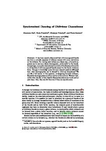
Parallelization has been studied broadly among discrete-event simulation. Basically, PDES parallelization techniques can be divided into optimistic and conservative techniques. To be effective, optimistic techniques, such as the Time Warp mechanism [11], typically require the assumption that communication is needed only rarely. In dynamic simulation, the derivatives of the variables in communication are usually non-zero and thus communication is usually needed in all sync points. Therefore, optimistic techniques fit poorly for dynamic simulation. Conservative techniques do not have this precondition, but their performance is poorer and less robust to changes in the simulation model. [1] Hence, it is not well advised to try to adapt any fine-grained parallelization technique designed for PDES to dynamic simulation. Common to most of the studies around parallel and distributed simulation for dynamic simulations is that there is a scheduler, coordinator, or some other central orchestrating unit apart from the simulators. This unit controls the execution of the simulations and typically mediates data between the simulations as well. In a study by Krzhizhanovskaya et al. [12], for instance, a job manager system monitors the utilization rates of each processor and gives jobs for idling processors. In a study by Brailsford et al. [13], a distributed simulation is coordinated by a middleware software component, through which all communication between the simulations occurs. A study by Santos et al. [14] presents a problem similar to the one in this thesis: a dynamic process simulation model is divided into multiple submodels which are simulated in a distributed fashion. In the study, a server–client architecture is used between a coordinating unit and the simulators, as is shown in Figure 2.1. The coordinating unit is waiting that all the simulators have reached the sync point, after which it transmits the variables in communication by using reads and writes. When a simulator has received the write command from the coordinator, it can start executing to the next sync point. The framework uses DCOM as the communication technology. The barrier synchronization technique used in parallel computing in general can be used also in synchronous simulation. In barrier synchronization, the multiple simulators run independently until they reach a common sync point which they may not pass before all of the simulators have reached that barrier. This technique as such does not specify a method for the communication between the processes. An example of barrier synchronization in simulation can be found in a study by Nicol and Liu [15]. The study presents a PDES framework with a hybrid synchronization mechanism with the barrier approach being one of the techniques used.
CHAPTER 2. COMPUTER SIMULATION TECHNOLOGY
11
Figure 2.1: The sequence diagram of the synchronization mechanism in the study by Santos et al. [14]
A co-simulation conducted in a parallel fashion leads to internal delays. This is well illustrated in Figure 2.1: A simulation does not obtain the result of the other until both of them have reached the sync point; this is contrary to a sequential co-simulation or any simulation with no parallelization. This delay can become an issue, for instance, in model based control: each output from the controller is given as input to the process model with a delay of one sync interval. This delay leads to error in the responses of the simulations and may lead to oscillation or, at worst, to the divergence of the whole co-simulation. In a study by Garcia-Osorio and Ydstie [16], a co-simulation synchronization mechanism is presented to tackle this problem: after the simulators have advanced to the sync
CHAPTER 2. COMPUTER SIMULATION TECHNOLOGY
12
point, the magnitude of the error is calculated. If the error is above a predefined maximum level, the iteration is re-run with a shorter sync interval. The error estimation and correction in detail is out of the scope of this thesis, though, and is thus not studied further. The time advance mechanism in a simulator is not necessarily always able to advance exactly to the next sync point but instead to some near point after the sync point. Interpolation is one technique that can be used to overcome this issue: the sync point value of a variable can be estimated with numerical techniques. [17] If, however, the time steps of the multiple simulations can be chosen to be multiples of each other, this issue can be avoided by choosing the sync interval accordingly.
2.4
Simulation Tools Used in This Work
In this section, the simulation environments used in this work are introduced and their real-life application areas discussed. First, a modeling language called Modelica is presented. Secondly, OpenModelica, an open source simulation environment for the Modelica language, is presented. Thirdly, the dynamic process simulator Apros is presented. Finally, the two simulators are compared with each other.
2.4.1
The Modelica Language
Modelica is an open standard modeling and simulation language developed in an international effort started in 1996. The Modelica Association, an international non-profit organization, has been developing the open standard since then. [18] The Modelica language is intended to be used in modeling the dynamic behavior of technical systems which consist of components from different domains. It can be used especially to model large, complex, and heterogeneous systems. It is an object-oriented high level language which can be used with systems that need high computational performance. [19] The Modelica language has three key differences with regard to most other simulation languages. These features are discussed in the following. First, in typical programming, modeling, and simulation languages, the functionality of a program is described with assignment sentences. When talking about physical equations, information is lost with such an approach. Modelica, however, is a declarative language using equations instead. The equations can be algebraic, differential, or discrete. As an example, the first order differential equation x˙ = −ax, a = 1 can be written in Modelica as is shown in the following:
CHAPTER 2. COMPUTER SIMULATION TECHNOLOGY
13
model SampleModel parameter Real a = 1; Real x; equation der(x) = -a * x; end SampleModel; To use equations implies that real-world physical objects can be modeled as such in the language. Therefore, the modeler does not have to consider in which way the equations are used, which would have to be done with languages allowing mere assignment. The generalization of the equations yields both simpler models and more efficient simulation. [19] [20] Secondly, most modeling languages are good at only a few technology domains. Modelica, however, can be used to model systems of different kinds. Systems such as electrical, mechanical, thermodynamic, hydraulic, biological, control, event, and real-time can be modeled and connected to each other to construct hybrid models. Moreover, Modelica is well suited for both low and high level numerical algorithms [21]. [19] Thirdly, Modelica is an object-oriented language with a general class concept. Added with the equation-based approach, it allows creating physically relevant and easy-to-use model components which are employed to support hierarchical structuring, reusability of components, and interoperability of ready-made model blocks. In other words, the class concept facilitates reusing and exchanging models and model libraries. [19] There are numerous implementations of the Modelica language available. The commercial Modelica simulation environments include Dymola, Vertex, Converge, The Modelica SDK, MOSILAB, SimulationX, AMESim, MapleSim, MathModelica, and Modelica Physical Modeling Toolbox for MATLAB. In addition to the commercial simulation environments, a number of non-commercial implementations exist as well. These include JModelica.org, Modelicac, OpenModelica, and SimForge. [18] In this thesis, only OpenModelica is discussed more deeply, even though the uses of some of the other environments are viewed in this subsection. As a general domain modeling language, the Modelica language can be used to model various types of technical systems. Industries applying the various Modelica environments include, but are not limited to, the following [22] [23] [24] [25]: • automotive, • shipbuilding, • aerospace,
CHAPTER 2. COMPUTER SIMULATION TECHNOLOGY
14
• robotics and mechatronics, • precision instrument development, • machine design, • electronics, • power plant industry, • oil and gas industry, • medical science, • system biology, and • education. A few examples of technical domains in which Modelica has been used are listed to give a scope of the divergence of the application area of Modelica. The examples are picked from customer references of Modelica tools [22] [24] [25] and are as follows: • electronic circuit simulation, • optimizing process control, • improving energy efficiency, • dynamic models development and analysis, • improve fault location techniques, • 3-D biomechanical modeling, and • evaluating different operation strategies.
2.4.2
OpenModelica
OpenModelica is an open-source environment, the purpose of which is to provide tools for building, compiling, and simulating models made using the Modelica language. It is intended to respond to both industrial and academic demands. The development and promotion of OpenModelica is supported by the nonprofit organization Open Source Modelica Consortium (OSMC). [26] [27] The OpenModelica system has both short-term and long-term goals. The short-term goals include developing an efficient interactive computational environment for the Modelica language and a rather complete implementation of the
CHAPTER 2. COMPUTER SIMULATION TECHNOLOGY
15
language. The main long-term goal is to have a complete reference implementation of the Modelica language, including simulation of equation based models and additional facilities in the programming environment. The long-term goals also include convenient facilities for research and experimentation in language design or other research activities. To achieve the performance and quality of the commercial products is not a goal of OpenModelica, though. [21] OpenModelica can be utilized as such to build and simulate Modelica models. In addition, since being free software, OpenModelica or parts of it can be integrated into existing systems as plugins or developed further by the user to better fit for the target system [21]. In the Simantics software platform, for instance, this sort of a plugin approach is utilized [28]. Scalability has been a key point in the development of OpenModelica for a couple of years [29] [30] [31]. The better the scalability, the larger models can be simulated. One goal of the experimental part of this thesis is a well-scalable implementation for both the OPC UA server and the synchronization of the server–server connection. Prior to the OPC interfaces implementation in OpenModelica, the OpenModelica Interactive (OMI) interface has been the solution for I/O in OpenModelica. The interface is very simple enabling only the most basic communication. After the initiation sequence, the OMI interface provides only the following functionalities: the simulation can be started, interrupted, stopped, or rewound to a specific time and parameter values of the simulation can be changed. In addition, OMI sends the values of the monitored parameters to the client after every simulation step. No browsing can be done through OMI, nor does it provide any metadata. Even though OMI utilizes TCP/IP protocol (Transmission Control Protocol / Internet Protocol), it uses strings of characters for all data. Thus, the performance of OMI is fairly poor if larger amounts of data must be transferred. [32] The importance of OpenModelica in industry is only starting to grow and is not nearly at the same level as its commercial counterparts. OpenModelica has been adopted in a larger scale only in academic usage. At the end of 2010 there were 18 members from industry and 14 from universities in OSMC [27]. As the amount of company members in the OMSC has been growing steadily [29] [30] [31], it could be predicted that industry will be increasingly adopting OpenModelica in the future. A couple of case examples in which OpenModelica has been used are as follows: • interactive simulations of technical systems in a virtual reality environment [33], • dynamic simulation of chemical engineering systems [34],
CHAPTER 2. COMPUTER SIMULATION TECHNOLOGY
16
• modeling Petri nets [35], and • fluid simulation and optimization [36]. As OpenModelica is open source software, it has been integrated as an extension to the simulation platforms Simantics by VTT [28], D&C Engine by Bosch Rexroth [37], and MathModelica Lite by MathCore [38]. In Simantics, OpenModelica is also utilized as the solver of the system dynamics tool.
2.4.3
Apros
Apros software is multifunctional software for modeling and dynamic simulation of processes and different power plants. It is intended to be used to model and simulate a whole power plant or other process. Apros is developed by Fortum (formerly known as Imatran voima) and VTT. It was first introduced in 1986 and has been developed further since then. The applications of Apros primarily include simulating power plants, both conventional and nuclear. It is also used in some other types of simulation such as batch production. In addition, users of Apros include automation suppliers, paper mills and solid oxide fuel cell system developers, among others. [39] Apros has also been subject for research: a number of theses which either utilize or study Apros have been written in Finnish Universities. Apros has several ways of communicating with external applications. The classic OPC DA is one of these methods: The Apros frontend implements the Adda interface. Adda is a proprietary interface with data access and simulation control functionalities. OPCDAKit is a dynamic-link library (DLL) included in Apros which maps the Adda interface to the OPC DA interface. In addition to the OPC DA interface, OPCDAKit implements the Simulation Control (SC) interface. The Simulation Control interface is used alongside with OPC DA to control the simulation. The Adda interface is described more thoroughly in Subsection 6.1.1. The application area of Apros is much narrower than that of Modelica and OpenModelica. Likewise with Modelica, the user base of Apros is global: there are Apros installations in 26 countries. These installations are used in development, research, analysis, operator training, and teaching. The most notable applications of Apros include the following [40] [41]: • combustion power plants, • fossil power plants, • thermal power plants,
CHAPTER 2. COMPUTER SIMULATION TECHNOLOGY
17
• nuclear power plants, • a fuel cell power plant, • a desulphurization plant, • a combined cycle gas turbine power plant, • a heat transport system [42], and • a ship engine room.
2.4.4
Comparison
Both OpenModelica and Apros are continuous dynamic simulation software. Even though OpenModelica has been intended for both industrial and academic usage, it has mostly been applied in the latter. Being open source enables OpenModelica to be used more freely. For instance, OpenModelica can be modified by end users to suit their needs better, used in education, or utilized in projects with less funding or which only want to test the feasibility of simulation as a tool. In contrast, Apros is mostly used in industry. It is clearly more suitable for larger projects with the focus being strongly on power plants. The strong points of Apros lie on process simulation. Apros has more extensive tools, algorithms, and libraries for, for instance, two phase flow phenomena at power plants. The tools have also been validated with real-world systems. The purpose-made tools include safety analysis, process design, training, and automation testing. The libraries have a wide set of components, such as pipes, valves, and pumps. In addition, Apros includes ready-made models of higher level components, such as heat-exchangers and reactors. [43] OpenModelica is a more general domain simulation environment than Apros. However, it does not yet fully implement all features of the Modelica language, let alone provide as efficient implementation as the most advanced commercial Modelica environments. On the other hand, OpenModelica has its strong points, too. For example, it provides more flexibility than Apros for own algorithm development. [44]
Chapter 3
OPC Interfaces OPC1 is an established interface specification for accessing field devices within control and automation systems; it has become a de facto standard throughout the industry [45]. OPC UA (OPC Unified Architecture) is the update specification for the classic OPC. It was developed to improve the classic OPC and to unify its functionalities under one interface. In this chapter, the OPC interfaces are presented: the classic OPC is discussed only briefly as the main focus of both this chapter and the whole thesis is on OPC UA. To avoid confusion, hereinafter in this thesis the term classic OPC is used to denote the set of OPC interfaces based on Microsoft technologies. The classic OPC is discussed in Section 3.1. When speaking of the OPC interfaces, both the classic OPC and OPC UA are included.
3.1
Classic OPC
The classic OPC is a set of specifications which defines a common interface for communication between different software packages and hardware devices. Its purpose is to enable the connection between factory floor devices and monitoring and control software applications in the domain of process control and manufacturing automation systems. In this section, the classic OPC is introduced: the technology upon which it is build is viewed and its applications are presented. Finally one of the classic OPC specifications, OPC Data eXchange, is introduced. OPC Data eXchange is a specification responsible for communication between applications on the same hierarchical level. 1 The
acronym OPC used to stand for Object Linking and Embedding (OLE) for Process Control. At present, it denotes open connectivity via open standards.
18
CHAPTER 3. OPC INTERFACES
3.1.1
19
Basis and Applications
From the beginning, the classic OPC was intended to be used to transfer realtime data between devices and display clients used in automation and control applications. The devices were usually programmable logic controllers (PLC) or distributed control systems (DCS). The display clients were supervisory control and data acquisition (SCADA) systems and human machine interfaces (HMI). Later the set of specifications was extended for other types of applications as well. The specifications define a standard set of objects, interfaces, and methods which enable vendor-independent interoperability between software and hardware [46]. Today, the classic OPC is the de facto standard for industrial integration and process information sharing [45]. [47] The classic OPC technology was built upon the OLE, COM (Component Object Model) and DCOM (Distributed Component Object Model) technologies developed by Microsoft. These technologies specify interfaces that can be used in passing objects between processes. The processes can be implemented in different programming languages and may be either located on the same computer or communicating over a network connection. The classic OPC is based on a server–client architecture. A typical use case for the classic OPC is that a software application acts as a client communicating with a separate server application. The server application is coupled with a hardware device enabling an access to the device. The client sends requests to the server which in turn processes the request and sends a response back to the client. These requests can be, for example, reading values or sending commands. [47] The original motivation for developing the classic OPC was to solve the so called “I/O driver problem”: without a common interface a special purpose driver must be written for each application–device pair, as depicted in Figure 3.1(a). With the classic OPC, each application and server needs to implement only one common interface (Figure 3.1(b)). In large and complex systems it would be practically impossible to operate with an individual driver for each such pair. The first and the most commonly used of the classic OPC specifications is OPC Data Access (OPC DA). It provides means for real-time data access to the underlying system behind the OPC DA server. In addition, it defines the general concepts of the classic OPC used also by the other parts of the specification. OPC DA can be seen as a solution to the original I/O driver problem. However, as the classic OPC was wanted to be used in different application areas, a set of new specifications was needed. One of these specifications is OPC Data eXchange. It is a specification which defines the communication between two OPC servers. OPC Data eXchange is described further in the next subsection.
CHAPTER 3. OPC INTERFACES
(a) Without OPC
20
(b) With OPC
Figure 3.1: Software applications are connected to hardware devices using either special purpose drivers or the classic OPC. [48]
3.1.2
OPC Data eXchange
OPC Data eXchange, abbreviated as OPC DX, is a specification part of the classic OPC. OPC DX is intended to be used for communication between applications on the same hierarchical level. Whereas OPC DA defines a server–client connection, OPC DX defines a communication method between two servers. It defines abstract services to configure the communication between one OPC DX server and one or more OPC DA and OPC DX servers. This subsection summarizes the key features of the OPC DX specification [49]. Figure 3.2(a) depicts a typical configuration between OPC DA servers and clients without any OPC DX capabilities: only server–client connections exist. With this connection configuration, any data sent from one OPC DA server to another must pass through OPC DA clients on the enterprise level. OPC DX adds the possibility to interconnect the servers on the same hierarchical level without an intermediate client. In Figure 3.2(b), the OPC DX servers can receive data from any OPC DX or OPC DA servers. Figure 3.3 depicts the high level architecture of an OPC DX server and its dependencies to other entities. The connection scheme consists of a source server, a target server, configuration clients, and ordinary OPC DA clients. The source server can be either an OPC DA or an OPC DX server, whereas the target server is an OPC DX server. The configuration clients are ordinary OPC DA clients with the capability to configure the target OPC DX server using the services defined in the OPC DX specification. Both configuration clients and ordinary clients can use the OPC DA interfaces of both the source and the target server in an ordinary fashion. Generally, multiple source servers may be connected to a target
CHAPTER 3. OPC INTERFACES
21
(a) Vertical integration using OPC DA [48]
(b) Vertical and horizontal integration of OPC DA and OPC DX servers and clients [48]
Figure 3.2: OPC DX adds horizontal server–server connection capability to the classic OPC. [49]
OPC DX server. For simplicity, an assembly with only one such server–server connection is discussed in the following. A connection between a source and a target server is established by the target OPC DX server. From the viewpoint of the source server, the target OPC DX server initiates the communication as any OPC DA client. The further operation is defined by the DXConnection items within the Connection database of the target server. Each DXConnection defines a connection between one source and one target item. A source item is an item inside the source server and a target item is the respective item inside the target server. The target OPC DX server is responsible for updating the target item when a change in the respective source item occurs. This is achieved by using the OPC DA read and subscription functionalities. Target items are shown to all OPC DA and OPC DX clients as any ordinary items within the target OPC DX server address space. Configuration clients can configure the connection between the target OPC DX server and the source server; they are used to map source items to target items and define the properties of such connections. These properties include,
CHAPTER 3. OPC INTERFACES
22
Figure 3.3: A connection between a source and a target item is established between classic OPC DX and OPC DA servers. [49]
among others, the update rate. Additionally, configuration clients can specify the organization of the DXConnection items in the address space of the target OPC DX server.
3.2
OPC Unified Architecture
Even though the classic OPC is widely adopted in industry, it has its weaknesses. OPC Unified Architecture (OPC UA) is a new specification whose purpose is to improve the classic OPC. OPC UA is not a new supplemental part for the already fragmented classic OPC specification but a unifying specification based on a new, different architecture. OPC UA is intended to be used wherever the classic OPC can be used and also in domains not suited for the classic OPC. OPC UA combines the functionalities of the different parts of the classic OPC under one specification adding new features as well. A completely new architecture has been adopted in OPC UA; the technology behind the classic OPC is becoming obsolete and does not allow all the improvements and features needed in the new specification. In addition, the base technology behind OPC UA has been chosen to enable forward compatibility with future technologies and to add new features. [50]
CHAPTER 3. OPC INTERFACES
23
In the following of this section, the OPC UA interface is introduced from a more practical viewpoint: the capabilities of the technology are discussed and compared with the classic OPC. In addition, the uses of OPC UA are considered: the applications, relevance, current status of the development, and wideness of the installment base of OPC UA are reviewed. The functionalities provided by the OPC UA interface are discussed in a more detailed fashion in Section 3.3.
3.2.1
Technical Differences between the Classic OPC and OPC UA
Even though the higher level functionalities of OPC UA are similar to the equivalents of the classic OPC, the technical differences beneath the surface are substantial. In this subsection, the most important technical differences between the classic OPC and OPC UA are examined on a higher level. The benefits that result for an end user are discussed in the next subsection. In addition to what is presented here, OPC UA introduces several fixes to the classic OPC and a number of new features. Instead of the DCOM technology, OPC UA is based on service oriented approach (SOA) paradigm: an OPC UA server exposes all of its functionalities as sets of services which can be used by OPC UA clients. The specification defines two different protocols for communication between a server and a client: XML WS (Web services), which is a widely used standard technology in communication between computers, and UA Native, a special purpose binary representation. The XML WS based protocol enables communication with any system that can communicate using Web services. UA Native enhances the speed of the connection at the expense of flexibility. [45] The data structure of OPC UA has been completely reformed to allow richer definition of the underlying system. The main differences are as follows. First, the nodes in the information models of OPC UA form a mesh network unlike the treelike structure used in the classic OPC. Secondly, the amount of metadata has increased vastly: the actual measurement data is described by a great amount of structural, semantic, and diagnosis data [45]. Thirdly, OPC UA has a class concept supported. Real-world items can be modeled as instances of classes (also known as objects). A similar approach is commonplace in object-oriented programming languages. The class concept allows custom types to be defined; even real-world objects such as actuators and sensors can be types [51]. A more detailed view of the data structure of OPC UA is discussed in Subsection 3.3.1. OPC UA emphasizes security. Unlike in the classic OPC, in OPC UA the security mechanisms are a fixed part of the communication. In OPC UA, security,
CHAPTER 3. OPC INTERFACES
24
reliability, and AAA (authentication, authorization, and accounting) are fully integrated into the specification. The level of security that is provided is sufficient to enable safe use over an Internet connection. With the security services implemented in the communication protocol, an application programmer does not need to pay much attention to it. [45] Nevertheless, for systems with tight performance requirements, it is still possible to switch the security off [52].
3.2.2
Advantages and Uses
The technical differences allow OPC UA to be used in a broader field of application areas than the classic OPC. In this subsection, the advantages of OPC UA are discussed from a more practical view. In addition, application areas of OPC UA are presented. Lastly, case examples of real-world applications are presented. The platform independence is one of the major benefits of OPC UA compared with the classic OPC. It enables OPC UA to be used in various platforms. The SOA architecture provides interoperability among many types of devices [45]. With a wide diversity of devices such as PLCs, intelligent modules, and even embedded devices supporting Web services, the potential installation base of OPC UA servers is much wider than that of classic OPC servers [53]. Therefore, OPC UA can be used in connecting not only a hardware device with a software application but also a software application to another software application or even a hardware device to another hardware device. The classic OPC can be used mainly in the plant floor network and the operations network of a factory for vertical integration. For any other communication, the classic OPC is quite impracticable. An advantage of OPC UA is its capability to integrate an overall information system of a company (Figure 3.4). This capability is due to the information model of OPC UA containing not only the values of the variables of the system but also a large amount of metadata describing the variables and their interdependencies in the system. Hence, the information acquired from the factory floor level can be utilized with ease even by higher level systems. With Web services as the basis of communication, this allows the overall information system of the factory to be integrated by using merely the OPC UA specification as the means of communication. This suggests that there can be a connection all the way from the factory floor devices through the process control systems (SCADA, HMI) and up to the process and business management systems, or even to systems in partner companies. [45] Figure 3.4 shows an example of a company information system communicating via the OPC UA interface. The PLCs, DCSs, and other data acquisition systems which control the factory floor devices are connected vertically with HMI and SCADA systems using the plant floor network. The plant floor network
CHAPTER 3. OPC INTERFACES
25
Figure 3.4: A typical information system of a company integrated with OPC UA
is integrated to the operations network through an aggregating OPC UA server. The purpose of the aggregating server is to provide higher level functionalities for upper level systems, such as manufacturing execution systems (MES), and expose them through the OPC UA interface. The operations network is in turn connected to the corporate network via another OPC UA server in order to provide the enterprise resource planning (ERP) systems with the desired functionalities. This server can also be utilized by external clients beyond an Internet connection. The platform independence and the elaborate information model alone do not ensure safe usage over networks. A data system of a company is often distributed also to the outside of a factory and may be controlled through an Internet connection. The use of Web services with efficient security procedures allows OPC UA to be used over network connections as well [45]. Hence, the connection between field devices and ERP systems can be established using ready existing multipurpose physical data connections. The amount of new features allows OPC UA to be used in a much wider area of applications. However, one of the goals in the development process of OPC
CHAPTER 3. OPC INTERFACES
26
UA was to retain all of the functionalities of the classic OPC [54]. Hence, OPC UA can be used practically wherever the classic OPC can be used. As the classic OPC has already a broad adopter base, it is also crucially important for the new specification that the migration to the new specification is made easy. Thereby, the backward compatibility between the two specifications has been ensured: a general-purpose middleware can be used to map the classic OPC interface to OPC UA interface [45]. Some real-world applications that already utilize OPC UA are presented in the following. These examples show the diversity of different application areas for which OPC UA is suitable: • In Alpha Ventus Offshore Windfarm, OPC UA is used in communication between the offshore windmills and the onshore monitoring and control systems. • xPAT (eXtended Process Analytical Technology) by ABB uses OPC UA and ADI to connect different types of analyzer devices. The system is already running at multiple customer sites. • Arburg uses OPC UA for high level application integration to VxWorks based PLCs which control molding machines. • In Miele, OPC UA is used for connection between HMIs and PLCs over an Internet connection. ¨ • In Swedwood Almhult, OPC UA is used for a basic communication within a factory PLCs and control systems. • NTE Systems uses OPC UA in energy monitoring and telecontrol in the energy system of multiple apartment houses over an Internet connection. [55] The adoption of OPC UA in real-world applications is only starting. Nevertheless, the aforementioned case examples show that there is a demand for OPC UA especially for installments in domains that are not very well suited for the classic OPC.
3.2.3
Disadvantages and Criticism
OPC UA has certain disadvantages compared with the classic OPC. Many of them are practical aspects which are due to the novelty and the extent of the new specification. One of the major concerns of the new technology, though, is the performance. The main performance issues concern data transmission and computational requirements.
CHAPTER 3. OPC INTERFACES
27
The transfer rates of data networks are constantly increasing but so are system requirements. With text-based XML messages used in transferring information, a substantial amount of the bandwidth is wasted from the information throughput viewpoint. Thus, transferring a certain amount of information is slower than with the classic OPC; with large quantities of data, the classic OPC can be roughly 20 times faster [50]. To remedy the slow transfer rate, the UA Native binary representation can be used. It provides much faster communication; the speed is nearly the same if not higher than with the DCOM technology [56]. Since the Web services technology is supported by many of hardware devices and software applications on the market, the use of the binary representation decreases interoperability and additional work is needed to interpret the binary representation. Hence, the UA Native protocol is at its best in applications with high information transfer requirements. The other performance issue is security. The practice has shown that security functions require a huge amount of processor time. The security can be turned off but then other practices need to be used to ensure the trustworthiness of the connection. A study by Cavalieri et al. [57] has concluded that using security can take 3 to 15 times as long as without security with small amounts of data. However, with data packages of more than one kilobyte the difference becomes much smaller: a connection with security takes only double of the time than a connection without security. For an application programmer, the new specification gives additional workload. Because of the extent and elaborateness of the specification, plenty of work has to be done even when creating small applications [58]. Even though the whole interface does not need to be implemented, the amount of work to achieve at least some minimal functionality is much greater than with the classic OPC. The OPC Foundation offers help by providing communication stack reference implementations in C, C#, and Java languages and sample client and server applications for C#. However, to build a software application upon a mere communication stack is very time-consuming. If C, C++, or Java is chosen as the language, using a commercial product to implement the required service sets is practically mandatory. Another issue is the installed base. Since OPC UA is a fairly recent specification, not as many products support OPC UA than the classic OPC. Thus, the interoperability cannot be fully utilized. There is no guarantee that OPC UA will gain a status similar to that of its predecessor. Only time will tell whether the new features will prove to be necessary enough that users of old systems will change over from the classic OPC to OPC UA and new systems will be designed
CHAPTER 3. OPC INTERFACES
28
with OPC UA as the means of communication. The current status of this topic is discussed in the next subsection.
3.2.4
Status and Future Development
In this section, the status of OPC UA is presented from two different viewpoints. First, the status of the specification itself is presented. Secondly, the status of OPC UA products available is viewed. The following presentation is based on the status of November 2011. The 13 parts of OPC UA are shown in Figure 3.5. All the core specifications, that is the first 11 parts, of OPC UA have been released. The parts 12 and 13 have been published as drafts only and are still under development. They are planned to be released in 2012. The released parts are also still being improved: clarifications as well as new features and enhancements are being added. [59]
Figure 3.5: The 13 parts of the OPC UA specification [60]
One of the targets for OPC UA is that it will become an IEC standard (International Electrotechnical Commission standard). The parts 1 through 6 and 8 have been released as the IEC 62541 standard. Parts 7, 9, and 10 are waiting for the final voting and will presumably be released in April 2012. The standardization of the last three parts is planned after 2012. [59]
CHAPTER 3. OPC INTERFACES
29
The companion specifications are an important element of OPC UA. These specifications provide standardized domain-specific information models which can be used to connect different applications within the information level of a factory. The four released companion specifications are DI (OPC UA for Devices), ADI (Analyzer Device Integration), FDI (Field Device Integration), and OPC UA for IEC 61131-3. [59] The number of OPC UA products available is increasing but is still only about a tenth of the number of classic OPC products. [48] However, the migration from the classic OPC to OPC UA is strong: most of the major OPC server and client vendors have changed to OPC UA [61]. For the first time in 2011, the amount of new OPC UA products was greater than that of new classic OPC products. At the moment, however, use cases in real environments are only starting. Nevertheless, automotive and chemical companies, for instance, are evaluating OPC UA in their use cases. [59] The classic OPC is the strongest competitor of OPC UA. It is estimated that the classic OPC is sufficient for about 80 % of industrial integration needs. Hence, there is usually no need to replace an existing classic OPC installation with an OPC UA equivalent. Typical applications for OPC UA are such for which a classic OPC implementation would be impractical or impossible. On one hand, these applications are such that need low level communication between field devices. On the other hand, OPC UA is much better suited for high level communication in factory management level systems with different operating systems and programming languages. [62] One of the goals of OPC UA is that it can be used for communication in all information levels in a factory. At the moment, many MES and ERP system vendors have implemented the OPC UA interface in their products. However, the problem is that currently the products on the lower levels are not yet provided with the OPC UA interface. [63] A framework for connecting a whole factory using OPC UA is being developed by companies such as Valio and Neste Jacobs. The target is that all connections between the numerous devices and applications in a whole factory will rely mainly on OPC UA. Both horizontal and vertical connections are being developed to replace the wide variety of communication interfaces used at the moment. [64] [65] One of the target application areas of OPC UA is embedded products. The platform independence of OPC UA has allowed installations for Windows, Linux, Android, and Apple iPhone and iPad, among others. For iPad, for instance, maintenance and configuration applications have been developed. [66] The OPC UA for IEC 61131-3 companion specification allows PLC–PLC connection between devices of different vendors, and thus no additional target PCs are
CHAPTER 3. OPC INTERFACES
30
required [63]. Companies such as Beckhoff Automation and Bosch Rexroth, among others, are currently developing OPC UA for IEC 61131-3 products and first of them are already available. [59] [61]
3.3
Functionalities of OPC UA – a Detailed View
In the previous section, OPC UA was compared with the classic OPC and its higher level properties were discussed. In this section, a more detailed view of the functionalities provided by the OPC UA interface is presented. The specification is very large and thus only the most relevant concepts of the interface are discussed. The emphasis is on areas which have greater importance for this work.
3.3.1
Address Space Model
For a deeper understanding about the functionalities the OPC UA interface provides, a short introductory to the address space model of OPC UA is given, along with a simple example. An OPC UA server contains an address space model which is a representation of the real system behind. The precise definition of the address space model can be found in the OPC UA Specification Part 3: Address Space Model [67]. The OPC UA address space model contains plenty of metadata which can be used to describe the properties of the various items and phenomena of the real-world system. As briefly mentioned before, a user can create self-made types to define the items in the system. These types define the general properties of the items they are associated with, not any specific data of a certain item. As an example, a ThermometerType type could be created to describe a general temperature sensor object and how it is linked with other parts of the system. The address space of OPC UA consists of nodes. Each node belongs to a node class (Variable, Object, or Method, for instance) specialized from the BaseNode class, as is depicted in Figure 3.6. For example, the ThermometerType type definition presented above would belong to the ObjectType node class since it describes the properties of an object. Based on the type definition, a thermometer object, belonging to the Object node class, can be instantiated to represent a temperature sensor in a real-world system. Nodes are in relation to other nodes via references. In this way, individual nodes can be linked together in the address space model in a similar fashion to how their counterparts are connected in the real world. For example, a thermometer object could be connected to its temperature variable. The relation could be defined as temperature being a component of thermometer.
CHAPTER 3. OPC INTERFACES
31
Figure 3.6: A node in the OPC UA address space model belongs to one of the node classes and has a fixed set of attributes depending on the node class. [51]
Nodes have attributes. Attributes serve as the descriptions of a given node. The use of attributes is strictly fixed and is defined by the node class, which prevents the user from creating or using custom attributes. For example, the temperature of a thermometer has a Value attribute (each variable has a Value attribute) which contains a floating point number, such as 22.0, expressing the result of the measurement. Figure 3.7 shows a slightly reduced view of the address space of the OPC UA server in the thermometer example. The address space has a root node, marked with a slash (/), of which type definition is FolderType; such nodes can be called folders. The root node organizes Objects and Types of which type definition is also FolderType. The Types folder contains all the type information needed to describe the system, including definitions for folders, thermometers, and temperatures. The Objects folder contains the objects and the variables of the system. In this example, there is only one object, namely thermometer, which in turn has a HasComponent reference to temperature. Both thermometer and temperature have
CHAPTER 3. OPC INTERFACES
32
Figure 3.7: The address space of the thermometer example
references to their definitions organized by the Types folder. The reading of thermometer is shown in the Value attribute of temperature. Even though not in full view, all the other nodes as well include a defined set of attributes. Even when the data structure of the address space is a graph, it can be flattened to a tree. Hence, the address space of OPC UA can model treelike structures as well as be viewed by software understanding merely treelike structures. The discussed thermometer example, for instance, can be flattened to a tree by making copies of such structures to which more than one reference is pointing. For example, the TemperatureType type is referenced by both temperature and ThermometerType nodes. Hence, two TemperatureType types need to be created, one for each node to be referenced by.
CHAPTER 3. OPC INTERFACES
3.3.2
33
Services
The functionalities that OPC UA provides are called services. These services are grouped into service sets. The services are described in more detail from an abstract point of view in OPC UA specification Part 4: Services [68]. In the following, the service sets are further grouped to correspond better to the functionalities shown to end users. • The Discovery, SecureChannel, and the Session service sets are used in establishing and maintaining the communication channel. The Discovery service set is used to obtain information about a server, the SecureChannel service set to open the connection between a client and a server, and the Session service set to handle the connection in the context of a session. These service sets are not discussed further. • The View and Query service sets can be used to browse the address space. These services enable discovering the objects, variables, and the methods in the address space in addition to their relationships and attributes. Using these services is somewhat analogous to browsing a file system of an operating system, the difference being that in this case the data system is a mesh network instead of a tree. The two service sets enable acquiring the real-time state of the address space. Additionally, they allow accessing the address space of a certain point in time in history. • The Attribute service set allows reading and writing the values of attributes, including the Value attribute. The service set allows also an access to the history of attributes and events. • The Method service set allows calling methods of objects. The most important methods in the scope of this project are simulation control and synchronization methods such as starting, interrupting, and continuing the simulation. • The MonitoredItem and Subscription service sets are responsible for monitoring the values of attributes. The monitoring can be based on either polling or events. A basic use case in the polling-based approach is that the OPC UA server publishes the value of an item being monitored at a user-defined interval. In an event-based approach, the value of the item being monitored is published to the client when a large enough change in the value has occurred. Additionally, there are a numerous other ways to use the service sets; these different modes of operation are not described further in this thesis.
CHAPTER 3. OPC INTERFACES
34
• The NodeManagement service set provides tools for adding and deleting nodes and references between them. In the scope of this project, this feature is not used and shall thus not be further discussed.
3.3.3
Exchanging Data
OPC UA does not include a data exchange specification similar to the classic OPC DX presented in Subsection 3.1.2. Neither does OPC UA specify a general scheme for server–server connection. The Aggregates part of the OPC UA specification [69] is the only one that defines one type of a server–server architecture. The main purpose of the Aggregates specification is to provide aggregate information from multiple sources of raw data. It defines a number of aggregate objects, functions, and data types. An aggregate server uses browse, read, and subscription to obtain data from its underlying OPC UA servers. It uses this data to calculate the values of the variables in its own address space. The aggregation is hidden from the clients: a client browsing an aggregating server does not implicitly know whether the server is an aggregating server. An aggregating server can be used, for example, to calculate the average value of a variable in time. Another example is to combine multiple variables in multiple servers to calculate the value of an aggregating variable. [69] Data exchange is intended to be based on server aggregation in OPC UA [69] [70]. However, using such an approach leads to different behavior to that of the classic OPC DX. The variables in the underlying server are shown as any nodes in the address space of the aggregating server. Any service call from an OPC UA client is passed through the aggregating server to the underlying server; that is, a read operation will read the variable in the underlying server and a subscription will monitor the real item on the underlying server. This is different from the classic OPC DX specification where the OPC DX server maintains local copies of the source items. Hence, any read in OPC DX server will read the value of the target item instead of acquiring the current value of the source item. Alternatively for the Aggregates specification, a proprietary architecture for data exchange can be developed. One way is to create an external OPC UA client to manage all communication between the servers. This method will lead to increased overhead in data transfer, though. Another way is to equip the OPC UA servers with ordinary OPC UA client capabilities. The servers can then communicate with each other without any excess middleware. In both of these solutions, variable values in the clients depend on the update rate they use to subscribe the variables in the other OPC UA servers.
CHAPTER 3. OPC INTERFACES
35
Little is currently being done to define a common specification for DX-like functionality in OPC UA by the OPC Foundation. At the writing of this thesis, nothing about the subject has been published. Nevertheless, there is intention to develop a common means for such data exchange in the future, at least to some extent. [71]
Chapter 4
Research Approach The experimental part of this thesis consists of designing and implementing the synchronization mechanism of the co-simulation environment and of testing its operation. This chapter introduces the items that are implemented and the tests that are used to evaluate the implementation. In addition, the tools and equipment used in this work are presented.
4.1
Design and Implementation
Creating the synchronization mechanism consists of the following subtasks: 1. Developing the OPC UA server interfaces for OpenModelica and Apros Within the co-simulation environment, the simulators communicate with each other solely via OPC UA. In addition, OPC UA interface enhances the simulators with a standard I/O interface. External applications can access and control the simulators via OPC UA. 2. Developing the OPC UA client interfaces for OpenModelica and Apros Within the co-simulation environment, the simulators can access and control other simulators using the OPC UA client. Additionally, the OPC UA client features allow OpenModelica and Apros to access and control applications implementing the OPC UA server interface. 3. Designing and implementing how multiple simulators are synchronized The design and implementation of the synchronization utilizes server– server OPC UA connection between Apros and OpenModelica simulations. The synchronization mechanism is designed to support any topology of simulators, even with cyclic connections. The most important aspect in the 36
CHAPTER 4. RESEARCH APPROACH
37
implementation is to develop the core components of the synchronization with a high performance in communication. 4. Designing and implementing how the connection between the simulators is managed The connection between the multiple simulations is configured and stored by an ad hoc proprietary software component embedded in the co-simulation environment. The connection can be configured through the OPC UA servers of the simulators. The chosen design and its rationale are presented in Chapter 5 on a higher level. In Chapter 6, the implementation is presented with a more technical viewpoint.
4.2
Tests
The design and implementation need to be tested in order to achieve the goals set in the introductory chapter. These tests are shortly described in this section. The objective of the tests is to ensure that the core functionalities of the implementation operate adequately. The more detailed descriptions of the tests, including the results and discussion, are presented in Chapter 7. In the basic control model co-simulation test, a simple co-simulation experiment is run in order to make a simple quality evaluation of the co-simulation environment. The response of the co-simulation is reflected against the response of the equivalent simulation done with only one simulator. The purpose of this test is to acquire some general knowledge on the effects caused by the division of the simulation model. The scalability test measures the scalability of the communication in the co-simulation mechanism implementation. In other words, the test aims at determining the maximum amount of items in the communication between the multiple simulators. The publish rate of the connection is also examined. The purpose of this test is to determine the feasibility of utilizing the implemented synchronization mechanism with larger co-simulation models. One goal of this work is to manage a co-simulation with more than two simulators. The topology of a co-simulation describes the interconnections between the multiple simulators. The multiple simulators can be connected together in a number of different topologies. Thus, to evaluate whether the co-simulation environment operates properly with multiple simulators, different topologies of simulator connections must be tested.
CHAPTER 4. RESEARCH APPROACH
38
The OPC UA server as such is not tested in this work. However, the scalability tests conducted with the co-simulation environment can be used to do certain conclusions about the plain OPC UA server as well.
4.3
Tools
In this section, the most important tools used in the experimental part of this thesis are presented. In addition to the software, the basics of the hardware are presented to help evaluate the test results. The computer on which the tests have been run is Intel Core™2 Duo CPU E8400 @ 3.00 GHz, 3.21 GB RAM. The implementation is running on Windows XP Professional Version 2002 Service Pack 3. OpenModelica is compiled with MinGW and Apros and the OPC UA and synchronization implementation with Visual Studio 8 and 9. The latest version of Apros is Apros 6 which has radical changes from the previous version. Instead of Apros 6, however, Apros 5.10.02 is being used in this work since the means for implementing the OPC interfaces in Apros 6 is yet undecided. The OpenModelica used in this thesis is version 1.7.0 [72], which was the latest stable version when the performance evaluations were started. The Unified Automation C++ SDK (software development kit) [73] version 1.3.0 is used to implement both the OPC UA server and client. The SDK provides implementations for, among others, the service sets of OPC UA, helper classes for frequently used functionalities, and security handling. The C++ SDK is a reasoned choice since the most parts of OpenModelica and Apros are written in C++ as well. In addition, the UaExpert OPC UA client by Unified Automation [74] is used for testing purposes.
Chapter 5
Design In this chapter, the design for the co-simulation environment implementation is presented. The different parts of the work are discussed on a higher level, different architectural approaches are compared, and the chosen architectural approaches are justified.
5.1
Qualitative Goals of the Design
In the introduction of this thesis, the main motivations and goals were presented. To meet those objectives, the design of the co-simulation environment needs to implement the following quality attributes: • Modularity and reusability The co-simulation environment implementation is divided into modules. This allows most parts of the implementation to be used in both Apros and OpenModelica. In addition, the implementation is connected with the underlying simulation application via a rather simple interface. Therefore, reusing the co-simulation environment implementation with other simulation software as well will be relatively easy. • Efficient connection The OPC UA server has short response times in the basic operations. This implies that, in addition to the plain OPC UA server, both internal and external communication in the co-simulation environment function efficiently. At least a fast publishing cycle of a subscription is needed, but also read and write operations should be efficient. At minimum, a publishing cycle of 200 milliseconds is required. In process simulation, a publishing cycle shorter than 50 ms is seldom needed [44] and thus achieving faster publishing cycles is not striven for. When the OPC UA 39
CHAPTER 5. DESIGN
40
connection is implemented efficiently, it can be used in target applications with soft real time constraints. • Scalability Both the OPC UA interface implementation and the whole co-simulation environment are scalable. It means that increasing the amount of items in communication does not affect the response time too severely. In this thesis, both the performance and scalability of the connection are evaluated. The details of the evaluation and results are presented in Chapter 7.
5.2
Architecture of the OPC UA Server
As mentioned above, the target is to use the OPC UA server implementation in both OpenModelica and Apros. Thus, it is reasonable to use a design similar to what is applied in Apros with the classic OPC server implementation (OPCDAKit): the OPC UA server maps the Adda interface of Apros to the OPC UA interface. In addition, the OpenModelica frontend is created to implement the Adda interface in OpenModelica. The OpenModelica frontend is basically an Adda interface implementation in OpenModelica. The Adda interface is discussed more thoroughly in Subsection 6.1.1. The OpenModelica frontend allows broader interoperability. In addition to the OPC UA interface, the Adda interface allows OpenModelica to communicate through the classic OPC DA and OPC XML-DA interfaces by using OPCDAKit and OPCXMLKit of Apros. Even though wrapper software which map the OPC UA interface to the classic OPC exist, they add an extra layer of abstraction in communication which potentially decreases the performance. Therefore, using these ready made OPC kits is considered beneficial. Two different architectural approaches for the OPC UA server were considered: The first alternative is to implement the OPC UA server as a DLL and integrate it as a fixed part of the simulators. The second alternative is to let the OPC UA server operate independently from the simulators and have its own means of communicating with the underlying simulations. These two solutions offer the following mutually exclusive properties: the former has high computational efficiency whereas the latter allows flexibility to modify the simulation model without disconnecting the OPC UA server from clients in OpenModelica. In the static solution depicted in Figure 5.1, the OPC UA implementation is similar to the classic OPC DA implementation already in use in Apros. Unlike in Apros, however, OpenModelica simulation models cannot be modified run-time
CHAPTER 5. DESIGN
41
and thus making changes to the model would yield to recompiling. The Adda interface is provided with functions that allow the simulation model to change while the server is operational but they can be utilized in Apros only. In addition to the OPC UA server DLL, the OpenModelica frontend needs to be implemented for the Adda connectivity in OpenModelica.
Figure 5.1: The static solution: Both OpenModelica and Apros incorporate an OPC UA server. Optionally, they can be connected to the OPC DA, OPC XML-DA, or the Simulation Control interfaces via the OPC kits.
The dynamic solution differs from the static solution by using a middleware component between the frontend and the OPC UA server. When a model change occurs, only the connection between the old model and the OPC UA server is cut after which a connection to the new model is established. One possible technique to implement the dynamic approach is to utilize the Aggregates specification, as is depicted in Figure 5.2: A static implementation of the OPC UA interface is first embedded in the two OpenModelica simulations. This static OPC UA connectivity is in turn used as the means of communication between the dynamic OPC UA server and OpenModelica. The OPC UA frontend is responsible for mapping the address space of the simulation model to the address space of the dynamic OPC UA server. When the dynamic OPC UA server is started, it establishes a connection to the OpenModelica simulation 1 via the OPC UA interface. When the model is modified and thus the OpenModelica simulation 2 generated, the connection to the first simulation is cut and a new one is created to the simulation 2. The two solutions described above have considerably dissimilar capacity demands as they emphasize the two mutually exclusive quality attributes:
CHAPTER 5. DESIGN
42
Figure 5.2: The dynamic solution can utilize the static OPC UA interface in communication between the dynamic OPC UA server and OpenModelica simulations.
computational efficiency and flexibility. When used in model based control in the destination process, there is no need to provide the ability to modify the model. When designing the co-simulation model, though, this feature would be needed by the modeler; with the static solution, the whole co-simulation cluster must be restarted every time a change is made to either any of the simulation models or to any connection between any pair of simulators in the cluster. On the other hand, the modeler does not necessarily need the computational efficiency which is needed in real-time control. Since efficiency limits flexibility and vice versa, both of the different architectural approaches should be implemented in order to support both of these use cases. Since the efficiency of the connection is the major goal of the OPC UA server, the static solution is implemented in this work. It is, however, conceivable that the static implementation can be reused to develop the dynamic solution later.
5.3
Synchronization
The literature is used to study the various different synchronization implementations utilized in co-simulation. However, only a small percentage of the studies on distributed, parallel, and cooperative simulation have been made around continuous simulators. To try to use any synchronization scheme created for PDES simulations is not very well advised. Hence, the various different ad hoc
CHAPTER 5. DESIGN
43
synchronization schemes for continuous co-simulation presented in literature are pondered. Three different ways to control the co-simulation cluster have been used in literature: 1. a centralized controlling unit to synchronize the simulators and mediate data between the simulators, 2. a centralized controlling unit to only synchronize the simulators, and 3. autonomous units that synchronize themselves and change data without external middleware. As mentioned before, a co-simulation problem similar to the one in this thesis has been presented by Santos et al. [14]. Hence, their design is taken as a starting point of the development. However, certain improvements to the synchronization mechanism are proposed in this thesis. The framework by Santos et al. employs a middleware client for synchronization and passing data. To decrease the amount of communication, the central orchestrating unit concept is discarded. Instead, the cluster of simulators is mostly self-organized: The simulators synchronize themselves by sending each other messages of their state. In this concept, each simulator is concerned that its own needs are met and that every one that needs it is satisfied as well; that is, the simulation can proceed if and only if all the required subscriptions from other simulations have been received and all the subscriptions have been published for all the subscribers. It could be argued that the design presented is not generally an improvement: A very large full mesh network of simulators may in fact suffer from scalability issues. This is because each simulator must send the information of its state to all of the other simulators one by one. Furthermore, if a set of variables are subscribed by more than one simulation, the same publish needs to be duplicated for each of the subscribers. Nevertheless, in the more likely use cases which employ a topology of simulators with only a few connected pairs of simulations, the amount of event notifications and subscription publishes is smaller. In addition, all latencies in interconnections are shorter since no additional intermediate steps exist in the communication. The barrier technique is chosen as the synchronization mechanism in this work. It is a technique which has been utilized in synchronous co-simulation in literature as well. The barrier technique has also been used in distributed Apros simulations. Figure 5.3 depicts a simplified version of the sequence diagram of the chosen design: When the simulation executables are launched, they create the
CHAPTER 5. DESIGN OPC UA Client
44 Simulation 1
Initialize
Simulation 2 Subscribe()
Initialize
Subscribe() Start()
Run(ti ck
)
Simulate
Publish()
Simulate
Publish() Run(ti ck) Simulate Publish() Simulate Publish() Run(ti ck)
Simulate
Publish()
Simulate
Publish()
... Figure 5.3: The sequence diagram of the synchronization mechanism
subscriptions to each other (Subscribe()). When the OPC UA client sends a start request (Start()) to either of the simulations (here Simulator 1), that simulator commands the other one to proceed till the next sync point (Run(tick)) and proceeds to the next sync point itself as well. When a simulator has reached the first sync point, it publishes the subscriptions (Publish()) and waits for the other one to do likewise. When the Simulator 1 has published and received its subscriptions, it sends the next start request (Run(tick)) to initiate the next iteration.
CHAPTER 5. DESIGN
45
The synchronization mechanism presented introduces two main sources of error. First, the error generated by the algorithms that evaluate the model numerically is in relation with the length of the sync interval. Secondly, a sync interval that is not a multiple of a simulation iteration causes error. Selecting a sync interval which is adequately short and a multiple of any simulation iteration will decrease the error. This sync interval selection is left on the responsibility of the end user.
5.4
OPC UA Client and Connection Configuration Management
To enable server–server communication, an OPC UA client is embedded in the OPC UA servers of OpenModelica and Apros. The client is used to receive variable values from other simulators and to control the other simulations. The connection between a pair of simulators needs to be defined; that is, what variables are transmitted and how their values are used. The design for configuring and storing this connection is explained in this section. OPC UA does not specify in detail a method that could be used for server– server connection. Thus, the configuration management definitions are strongly based on the classic OPC DX interface introduced in Subsection 3.1.2. To efficiently acquire data from other simulations, subscription is used. It could be argued that data could be mediated by using the write functionality instead, as it is done in the design by Santos et al. However, a number of reasons favor subscription: First, if write was used, utilizing the design with third party OPC UA compliant applications would be much more difficult, since they would need major modifications. Secondly, subscription is used in the OPC DX specification as well. Thirdly, the current way of communication between multiple Apros simulators is based on a similar design. Only a very simple OPC UA client is needed in this work: in addition to establishing a connection, only subscriptions and methods are used. As creating a client which could use other applications with an OPC UA server is not a goal of this thesis, the client is designed to be used in co-simulation only. Nonetheless, the client is implemented in a way which allows it to utilize any OPC UA compliant application in the co-simulation environment with only a few simple additional functionalities implemented into the included application. Since the client implementation itself has few noteworthy details, it is not discussed further in detail.
CHAPTER 5. DESIGN
46
A connection configuration manager is embedded in the synchronization mechanism. To allow early testing with the whole synchronization mechanism, the target is to create a format which can be easily modified both with a text editor and via OPC UA. The numerous advantages of XML make it a self-evident choice for the technology to store the configuration. Since the focus of this work is to create the co-simulation environment, the connection configuration manager is designed to be utilized mainly in synchronous simulation. The potential of the rich address space model of OPC UA is not utilized much in the connection configuration. The main reason for not doing so is that it would not help achieve the main goals of the thesis. Additionally, one reason why a more expressive representation is not implemented is that the DX-like functionality in OPC UA is yet undefined. An alternative – not necessarily a competing one but more of an enhancement – for defining the connection information would be to use the abilities of the rich information model of OPC UA: The address space of the server containing the source items could be embedded in the address space of the OPC UA server where the target items lie. All the connections could then be modeled as references between the source and target variables. However, this approach introduces two major issues: First, only the most basic information about the connection can be expressed with such a reference. This information could consist of the locations of the source and target variables and of the server in which the source item lies. Any other information must anyway be presented with some other means in the address space. Secondly, it seems that little or no advantage could be achieved for the main objective of this thesis by developing such a design.
Chapter 6
Implementation In this chapter, the implementation is discussed in a more detailed fashion. First, the plain OPC UA server implementation is introduced. After that, the synchronization implementation is presented. Finally, the connection configuration manager is viewed.
6.1
OPC UA Interface in OpenModelica and Apros
The OPC UA server is implemented into the simulators similarly to the classic OPC interfaces are implemented in Apros. The OPC UA server is a DLL which communicates with the simulation via the Adda interface. First in this section, the Adda interface is presented in detail. Secondly, The OpenModelica frontend implementation is described shortly. Finally, the details of the OPC UA server implementation are discussed.
6.1.1
Adda Interface
As mentioned earlier, Adda is the interface used in Apros for external I/O. The Adda interface is utilized by the OPC kits to enable the classic OPC connectivity in Apros. The Adda interface is a relatively small definition being merely a collection of functions which can be used by external software to communicate with simulator software. Adda does not, however, specify as comprehensive a communication solution as OPC UA. The Adda interface is developed for communication quite similar to what can be achieved by using the classic OPC DA interface. In addition, a set of commands has been added for simulation control purposes. A more detailed view of the Adda interface can be found in its technical report [75]. 47
CHAPTER 6. IMPLEMENTATION
48
The address space of Adda has much in common with the classic OPC. Adda as well can be used to process treelike structures only. The address space behind the interface consists of branches and items. A file system analogue for a branch is a folder and for an item a file. The sole functionality of the branches is to organize items. An item consists of the value of the item and a small amount of metadata describing the item. In general, however, little metadata of the underlying simulation is available through Adda. The Adda interface consists of functions of four different types: • The first set of functions is the utility functions, the main purpose of which is to initiate and terminate the connection. • The second set of functions is for browsing the underlying database: the functions provide a similar means of scanning the database than what is achieved by using the OPC interfaces. • The third set of functions is for data access. To be exact, these functions allow merely writing data to the simulator; reading a value is executed by accessing the data directly by using a pointer to the item inside the simulator. In addition, the data access functions incorporate functions used in the reverse direction: the simulator can inform of a change either in the simulation model or in a value of a variable in communication. • The fourth set of functions is for simulation control: the means to start, pause, and continue the simulation are provided among other functionalities. This set of functions adds general support for events, too. An additional layer of abstraction drops the performance of the system a certain amount. Adda is a very lightweight interface, though. Since Adda enforces no additional copying of values or using of complex data structures, it does not add much computational overhead to the communication.
6.1.2
OpenModelica Frontend
To allow the OPC UA server to be connected to OpenModelica, the Adda interface is implemented into OpenModelica. This implementation is referred to as the OpenModelica frontend. Since all of the functionalities of Adda are not necessarily needed in this work, only a subset of the functions of Adda is implemented. The OpenModelica frontend implementation is available in OpenModelica SVN [76]. The Adda interface provides little support for representing metadata which gives limitations to utilizing the structural representation of Modelica. Thus,
CHAPTER 6. IMPLEMENTATION
49
for instance, the class information about the objects in the model cannot be transferred via Adda. Even then, the provided metadata is sufficient for all basic operations needed in this work. In addition to the Adda interface implementation, certain COM interface initialization functions have been implemented into the frontend. These functions allow the implementation to be validated against the classic OPC DA implementation, OPCDAKit. For that purpose, a few Adda functions unused by the OPC UA server are also implemented.
6.1.3
Implementation Details of the OPC UA Server
In this section, the main details concerning the OPC UA server implementation are further discussed. Basically, the implementation is a mapping from the Adda interface to the OPC UA interface. The functionalities of the OPC UA interface are implemented only to a certain extent. With the restrictions caused by the Adda interface, it would not be even possible to implement a system supporting all the functionalities provided by OPC UA. In the scope of this work, the target is to implement basic functionalities to enable browsing the address space, reading and writing values, and subscribing for variable values and events. The Adda interface is strongly based on the classic OPC DA interface which has many similarities with OPC UA. Nonetheless, there are significant technical differences as well, which leads to difficulties in the implementation. In addition, the OPC UA interface needs to be slightly modified for a desired outcome. The modifications are also described in this subsection. The address space of the underlying simulation is mapped to the address space of OPC UA in a straightforward manner. The Adda interface can handle only trees with branches and items. Hence, the address space of the simulation is mapped to the OPC UA address space as a tree as well. An example OPC UA address of an OpenModelica simulation is presented in Figure 6.1. The proprietary part of the address space is the Simulation object. Objects and components of OpenModelica and Apros are presented hierarchically as objects and variables under the Simulation object. The simulation control functions of Adda responsible for starting and interrupting the simulation are mapped to OPC UA method calls in a straightforward manner. The four methods implemented are Start(), Stop(), Step(), and Run(seconds): • Start() starts the simulation, • Stop() pauses the simulation at the end of the ongoing iteration,
CHAPTER 6. IMPLEMENTATION
50
Figure 6.1: An example OPC UA address space
• Step() advances the simulation one iteration, and • Run(seconds) starts the simulation and pauses when the time given as a parameter has elapsed. The simulation control methods are placed under the Simulation object in the OPC UA address space. Adda interface uses a grouping methodology similar to that of the classic OPC. According to the performance evaluation made for the classic OPC DA by Iwanitz and Lange, the performance of the communication does not depend much on the amount of groups used in communication [77]. Hence, in this implementation, it is seen reasonable to use only one group for all items in communication when communicating through Adda. Instead of real time, the clock of the OPC UA server advances at the same rate than the simulation time. To be precise, the time of the OPC UA server is server initialization real time added with the simulation time. Even though
CHAPTER 6. IMPLEMENTATION
51
a real time clock is utilized in the internal behavior of the server, all external behavior is based on the simulation time. Thus, all timestamps, subscriptions, and events are dependent on the simulation time. This approach is similar to what is already in use in the classic OPC implementation in Apros. A possible risk in this approach is that third-party software may not function supposedly. However, not any problems have been discovered with any OPC UA or classic OPC third party software products due to this modification. The OPC UA specification states the following: The sampling interval is the fastest rate which an OPC UA server uses to sample its underlying source. Moreover, the sampling interval is the fastest rate at which an OPC UA server serves its clients. [68] The consequences of these definitions are shown in Figure 6.2; a change in the underlying system is visible after a varying delay. To achieve deterministic behavior, this uncertainty is unacceptable since any additional delay affects the result of the co-simulation.
Figure 6.2: Delay in detecting a change in the real system [68]
Due to the abovementioned nondeterministic nature of OPC UA, certain parts of the SDK used in the OPC UA server implementation are based on polling. This is harmful for high performance since the polling of values creates additional overhead to the communication. However, since modifying the SDK to work asynchronously would require enormous amounts of work, the polling based approach is mostly used with the exception of subscription publishes: The target is that a change of data at simulation time t is sampled and published at time t as well. Thus, a subscription is published only after the simulation has
CHAPTER 6. IMPLEMENTATION
52
paused and the sampling is completed. The target is achievable, since the clock of the OPC UA server is stopped during this whole procedure.
6.2
Technical Details of the Synchronization Mechanism
To synchronize the multiple simulations, a piece of software labeled as the synchronizer is implemented as a part of the OPC UA server. If the synchronous simulation is enabled in the OPC UA server, the synchronizer is started after the OPC UA server has been initialized. The synchronizer is responsible for controlling the underlying simulator and communicating with the other simulators in the cluster using an OPC UA client. In this thesis, the following definitions apply: • An OPC UA client which subscribes synchronously data from simulation S is a subscriber of simulation S. • An OPC UA server which is subscribed synchronously by simulation S is a subscribee of simulation S. Even though this thesis is concerning synchronized simulators within a cluster, these definitions apply to any software that acts similarly. For example, if the co-simulation environment was further developed, simulated DSCs or other applications could be embedded in the synchronization. These applications can be either external or internal to the actual co-simulation cluster. In the contrast, when speaking of external OPC UA clients that subscribe to any OPC UA server within the co-simulation cluster, the term external OPC UA client is used. These clients do not subscribe the co-simulation servers in a synchronized manner, or if they do, they use some synchronization scheme of their own. The synchronization is based on a fixed time step; that is, all of the simulators in a cluster have identical sync points and the length of every sync interval is a constant. The synchronizer within each OPC UA server advances the underlying simulation to the following sync point by calling run(seconds) of the Adda interface with the sync interval length as the attribute. The synchronizer uses two OPC UA methods to communicate with other simulations. One of these methods is InitSync(U RL, syncInterval, clusterId), where U RL (uniform resource locator) is the URL of the caller, syncInterval the sync interval of the co-simulation cluster, and clusterId an identifier to define which connection configuration is used. When a simulator wants to join a co-simulation cluster and make subscriptions to other simulators, it
CHAPTER 6. IMPLEMENTATION
53
calls the InitSync method of each simulator to which it wants to subscribe. The other method is ProceedToSync(simulationT ime), where simulationT ime is the end time which the simulation is allowed to execute to. When a simulator in the cluster has received all subscribed values of one of its subscribees and acted accordingly, it calls the ProceedToSync method to inform that subscribee that it may continue the simulation. When that subscribee has received a ProceedToSync call from all of its subscribers, it may actually proceed to the next sync point. The user of the co-simulation is provided with the following four methods: RunSecondsSync(time), StartSync(), StepSync(), and StopSync(). A user can call the RunSecondsSync method to simulate the co-simulation for the length of time. When the RunSecondsSync method is called for one simulator, that simulator calls ProceedToSync of its subscribees, which in turn call ProceedToSync of their subscribees, and so on. Thus, the whole co-simulation cluster is started with only one method call by the user. The three other methods, StartSync, StepSync, and StopSync, are basically only variations of RunSecondsSync with the following relations: • StartSync() = RunSecondsSync(∞), • StepSync() = RunSecondsSync(next syncPoint), and • StopSync() = RunSecondsSync(0). As said before, the synchronization is based on autonomously operating simulator units. Each such unit is responsible for ensuring that its subscribed items are received and that its subscribers have received their subscribed items as well. The operation of a single simulator is presented in detail in the two activity diagrams: The independently operating OPC UA server subscription management thread is depicted in Figure 6.3. The synchronizer thread is depicted in Figure 6.4. The two activity diagrams are explained in detail in the following. All the method parameters have been omitted from the notation. When the OPC UA server is used in the synchronized simulation, the subscription management operates as follows: When the OPC UA server is started and a new subscription is created, the initial values of the variables are published and an event is sent to confirm that the publishes have been performed. When the simulation is started, the thread stays on hold. When the simulation reaches the first sync point it stops and notifies the subscription thread to publish the values and the event. When the simulation is continued, the cycle is repeated. All subscriptions of each subscriber operate similarly. The synchronizer thread operates as follows. When the synchronizer is started, it connects to all of its subscribees and creates the subscriptions. Af-
CHAPTER 6. IMPLEMENTATION
54
Publish subscribed values
Publish subscribed events
Sync point reached
Wait RunSeconds(syncInterval) Running
Figure 6.3: OPC UA server subscription thread activity diagram
ter that, it starts to receive InitSync() calls from other simulators. For each InitSync(), the synchronizer adds the caller to its subscribers list. After the initialization phase, the synchronizer waits for a start command from either a user (RunSecondsSync()) or from another simulator (ProceedTo()). If it has no subscribers, it can be started only by a user. After a start command, the synchronizer goes into the loop where it tests whether it can advance the simulation. In the loop, the synchronizer first checks whether it has called ProceedTo() of each of its subscribees to allow them to continue to the next sync point. If not, it does so, assuming that the end time given by either the user or by another simulation has not been reached. After it has made the ProceedTo() calls, it waits that all of its subscribers in the subscriber list allow it to continue by calling its ProceedTo(). After they have done so, the synchronizer can enter the final phase of a co-simulation iteration. In the final phase, the synchronizer writes the subscribed variable values to the simulation. After that, it calls run(syncInterval) of the Adda interface to run the simulation till the next sync point. The synchronizer waits for an event from the simulation to signal it that the sync point has been reached. After that, the synchronizer waits until it has received a subscription publish from every one of its subscribees; when all subscribees have sent an event, the synchronizer knows that all of the variables subscribed have been sent as well. In the meanwhile, the
CHAPTER 6. IMPLEMENTATION
55
Connect to all subscribees, Call InitSync() of each subscribee InitSync()
RunSecondsSync()
Initiate synchronization, Add a subscriber ProceedTo()
InitSync()
RunSecondsSync()
Have ProceedTo()’s been sent? No RunSecondsSync() Is there time left? Yes
Yes Send ProceedTo()’s to all subscribers
all subscriptions received
No Have I received a ProceedTo() from each subscriber? No ProceedTo()
Yes Write subscribed values to the simulator
Wait for ProceedTo()’s Continue the simulation sync point reached Pause the simulation, (Serve the subscribers)
Figure 6.4: Synchronization mechanism activity diagram. The method parameters are left out of the notation.
subscription thread is publishing subscriptions to the subscribers. When all subscriptions have been received, the synchronizer can start the loop again.
CHAPTER 6. IMPLEMENTATION
56
Even though the simulators have seemingly similar hierarchies with each other, there is always at least one so-called master simulation in a co-simulation cluster. The master simulation is a simulation which is controlled by a user with the RunSecondsSync method. Thus, the only difference between a master and a regular simulation is that a master simulation is responsible for running the whole co-simulation according to the user’s instructions, that is, to start and stop the simulation when desired by the user. In many of the typical use cases, the master simulation can be chosen arbitrarily. However, a simulation which cannot excite the whole cluster by recursive ProceedToSync method calls cannot be chosen as the sole master simulation. Moreover, certain co-simulation topologies need multiple master simulators. As an example, the two simulators in Figure 6.5 that have no subscribers within the cluster must both be masters. This is because the simulation in between them does not subscribe to either of them and thus does not call ProceedToSync of either of the other two simulators. M
M
subscribe
subscribe
Figure 6.5: The simulations marked with M are masters in the co-simulation cluster.
External OPC UA client applications can use the OPC UA servers of the simulators between the sync points as well. However, the chosen implementation approach has its downsides on this connectivity: As said, the sampling implementation is based on polling. Thus, if the simulation runs faster than the sampling polls the simulator, the values within the OPC UA server cache are not updated at every iteration and thus cannot be published to the clients.
6.3
Connection Configuration Management
In this section, the connection configuration manager is presented. Its function is to store and utilize the connection configuration and provide the ability to browse and modify it via OPC UA. First in this section, the address space model of the connection configuration is introduced. Secondly, the methods in the address space for modifying the configuration are viewed. Finally, the XML schema developed to save the configuration is presented.
CHAPTER 6. IMPLEMENTATION
6.3.1
57
Address Space
The connection configuration is visible through the OPC UA interface as a part of the address space. The structure of the address space model is strongly influenced by the address space model of the classic OPC DX specification depicted in Figure 6.6. The Status branches and other details of minor importance have not been implemented. Otherwise, all that is presented in Figure 6.6 applies to the implementation of this work.
Figure 6.6: The DX branch of the address space in a classic OPC DX server [49]
A sample address space is shown in Figure 6.7. In this figure, the DX object is expanded recursively. Moreover, even when not shown in the figure, all of the objects under the DX object have their respective TypeDefinition nodes within the Types folder. The address space model of the connection configuration manager is explained using Figure 6.7 as an example. The DX object is placed on the same level with the Simulation object. Likewise with OPC DX, the DXConnectionsRoot and SourceServers objects are placed under the DX object. In addition, the Synchronization object is under the DX object as well.
CHAPTER 6. IMPLEMENTATION
58
Figure 6.7: An example address space of the DX object
DXConnectionsRoot contains folders and DXConnection objects. A DXConnection object is similar to the DXConnection item defined in the OPC DX specification with only minor modifications: the DXConnection object is supplemented with the ItemID and namespace index of the source item as well as the
CHAPTER 6. IMPLEMENTATION
59
namespace index of the target item. These new parameters allow an item on a source server to be accessed in two alternative ways: The conventional way is to first browse the address space of the source server to acquire the ItemID of the desired item. After that, the item can be read, written, and subscribed. The new way is to use the ItemIDs provided by the connection configuration manager to directly access the desired items without needing to first browse the address space to find them. The latter way enables an easier start-up of the co-simulation cluster. Only this approach is implemented in this work. The SourceServers object contains all the source server objects. A source server object is defined with two string variables: name and URL. A source server is uniquely identified by the value of the name variable, and the value of the URL variable is the endpoint URL of the source server. The Synchronization object consists of the methods which are used by other simulators and external OPC UA clients to control the simulation. In addition to the methods, the synchronization object contains the TickLength variable which denotes the length of the sync interval. In addition to what was presented above, the address space contains methods that allow the configuration to be modified via OPC UA. These methods are discussed in the following subsection.
6.3.2
Configuring the Connection via OPC UA
Configuring the connection via the OPC UA interface is done with methods. With these methods, a user can • change the length of the sync interval, • add, modify, and delete source servers, and • add, modify, and delete DXConnections. The methods implemented are based on OPC DX services. The whereabouts of the methods within the OPC UA address space are shown in Figure 6.7. All the methods with their arguments shown are presented in Appendix A. The length of the sync interval can be modified with the SetTickLength method. This method is placed under the Synchronization object. A new source server can be added by using the Add method under the SourceServers object. An existing source server can be modified with the Modify method under that source server object. If an empty string is entered as a parameter, it is interpreted that the parameter is not to be changed. A source server which is not referenced by any DXConnection can be deleted with the Delete method.
CHAPTER 6. IMPLEMENTATION
60
A new DXConnection can be created by using the Add method under the DXConnectionsRoot object. The created DXConnection is added under the specified path under DXConnectionsRoot. An existing DXConnection can be modified with the Modify method under that DXConnection object. Again, if an empty string is entered as a parameter, the parameter is not changed. A DXConnection can be deleted with the Delete method. The implementation of this work does not allow changing the connection between the simulators in run-time. The methods described above alter only the XML configuration file used to store the connection configuration. Thus, to modify the connection, the co-simulation cluster must be restarted.
6.3.3
Storing the Configuration
The connection configuration is stored in an XML file. One configuration file can be used to define all connections of a whole co-simulation cluster. Alternatively, one configuration file for each simulator can be used to define only the connections from that simulator, that is, the subscribees of the simulator and the related DXConnections. The configuration file defines which server–server connections exist and what source item–target item connections they include. The format of the connection configuration is defined in the XML Schema file presented in Appendix B. An example XML configuration file based on the Schema is presented in Appendix C. All of the connections in the co-simulation cluster are defined in that one file. In this example, all the critical definitions are filled; the attributes and elements left blank are visible in the OPC UA server address space but contain no functionality whatsoever. The contents of the example XML file are explained in the following. The first noteworthy element in the configuration file is the Tick element, which denotes the sync interval. It has Length as a subelement. The Tick element is common for all connections in a co-simulation cluster since the whole cluster operates with a same sync interval. The server–server connections are defined with the Connection elements. A Connection element defines a subscriber–subscribee pair of simulators connected together and the DXConnections of that connection. Furthermore, each Connection has an Enabled element, which defines whether the Connection is included in the parsing of the XML file. The DXConnections are grouped based on their subscriber–subscribee pairs. The DXConnection elements have the parameters and attributes given when creating the DXConnection. As an exception, SourceServerName is not included as an attribute of a DXConnection element since it is already evident form the location of the DXConnection element in the XML file.
Chapter 7
Testing and Evaluation In this chapter, the implementation presented in the previous chapter is evaluated. In Section 7.1, the different tests are described in detail and their results are presented and analyzed. In Section 7.2, the results are discussed and reflected against the goals of the experimental part of this thesis.
7.1
Tests
Three different tests are conducted with the synchronization mechanism. The tests help evaluate the feasibility of utilizing the co-simulation environment implementation in real-world process simulation applications.
7.1.1
Basic Control Model Co-simulation
As stated earlier, Apros and OpenModelica excel at different areas. A likely use case for co-using the two is to simulate a process with Apros while OpenModelica is simulating a controller for that process. In the planning phase of this thesis, a target was to evaluate the co-simulation environment with a real-world process model of an industrial partner. Since this collaboration did not succeed, only a very simple test case to evaluate the implementation was created in this thesis. The purpose of the basic control model co-simulation test is to briefly evaluate the synchronization mechanism: the aim is to examine the effects caused by the division of a simulation model into two submodels which are run in separate simulators. In particular, the target is to illustrate the influence of the internal delays emerging in the co-simulation model due to the latencies in communication between the simulators. In this test, two similar simulations are run. The first simulation is run in Apros only and the second one as a co-simulation of Apros and OpenModelica. A sync interval of 200 ms is used in the co-simulation, the step length of both of 61
CHAPTER 7. TESTING AND EVALUATION
62
the simulations is also 200 ms. The simulation experiments are based on the Apros model depicted in Figure 7.1.
Figure 7.1: A PI controller controls a valve.
In the model, a PI controller (proportional-integral controller) controls an actuator which opens and closes a control valve. The valve is connected to two pipes through which liquid flows due to the different pressures and elevations in the endpoints of the pipes. The PI controller measures the flow in the upper pipe and, based on the measurement, opens or closes the valve to make the flow through the pipe equal the desired setpoint value. The input of the model is the setpoint value of the PI controller and the output is the actual flow through the upper pipe. In this test, two experiments are run. In the first experiment, the Apros model above is run as such. In the other experiment, the PI controller block is replaced by an OpenModelica equivalent (Modelica.Blocks.Continuous.LimPID). The OpenModelica PI controller is tuned similarly to the PI controller in Apros. In both of the tests, the system is excited with the same step input ( SP =
0 , when t < 5s , 5 , when t ≥ 5s
CHAPTER 7. TESTING AND EVALUATION
63
where SP is the setpoint of the PI controller and t the simulation time. The outputs are plotted to analyze how the division of the model between the two simulators affects the response of the simulation in the chosen co-simulation environment design. The output of the Apros simulation is depicted in Figure 7.2, as well as the input signal. The PI controller is tuned to follow the input relatively fast. Thus, as can be seen, the output follows the input rapidly with a 15 % overshoot and oscillates only slightly.
Figure 7.2: The step response of the simulation with the whole model simulated in Apros
The output of the co-simulation is presented in Figure 7.3, as well as the input signal. Even when a similarly tuned PI controller is used, the output differs drastically from the first simulation: the output starts to rise later, overshoots, and oscillates a considerably greater amount. As stated in Section 2.3, dividing the model into submodels may cause error in the outcome of the simulation. The different behavior of the two simulations is mostly due to this error. When the setpoint is changed in Apros, it needs to be transmitted to OpenModelica as the input of the PI controller. The output of the PI controller is computed in OpenModelica, after which the output is mediated to Apros. The same applies with the measurement signal for the controller.
CHAPTER 7. TESTING AND EVALUATION
64
Figure 7.3: The step response of the simulation with the process simulated in Apros and the PI controller in OpenModelica
Hence, it takes two sync intervals prior to either of the PI controller inputs in Apros can affect the PI controller output in Apros. Since the sync interval of the co-simulation is 200 ms, an additional delay of 400 ms emerges. This causes the controller to react more slowly to given inputs which leads to the differences described before: The dead time prior to the rise of the output is increased by the 400 ms. The overshoot is more severe since the controller receives the information of reaching the setpoint only after the output has already 400 ms ago passed the setpoint. The oscillation has a similar cause as well. The result of this test raises the question of how to prevent or decrease the error generated. A straightforward solution for decreasing the error is to shorten the sync interval or to use a slower tuning in the controller. Since the error related issues do not belong to the scope of this thesis, this issue is not studied further.
7.1.2
Scalability
The purpose of the scalability test is to determine how the performance of the co-simulation environment is affected when increasing the amount of items in
CHAPTER 7. TESTING AND EVALUATION
65
communication between the multiple simulators; the processing time needed for the synchronization is measured in these tests. The target is to determine the amount of data that can be exchanged between the simulators in a cluster and how short sync intervals can be used. The test setup is based on the requirements of real-time process simulation, yet the results can be applied to other types of simulation as well. It must be stressed that the sample sizes used in the tests are too small to accurately estimate the performance of the system. However, since the test environment has quite a many unknown factors as well, an accurate analysis would be difficult even with more thorough testing. In addition, since the target of the tests is to give only a rough estimate of the capabilities of the system, the small sample sizes can be justified. In process simulation, it is typically sufficient to use a step length of 200 ms. In some rare occasions, 50 ms step length may be needed. On the other hand, for some processes even a step length of one minute may be sufficient. [44] Thereby, these tests examine the behavior of the co-simulation environment with the sync intervals of 50, 200, and 1000 ms. For consistency, however, the step length of 50 ms is used for all individual simulators. Even when a process simulation model may consist of even millions of variables, a common use case is that not all of them need to be monitored by external applications [44]. The tests in this subsection examine the behavior of the co-simulation environment with up to 3000 variables per simulation in communication; thus, a co-simulation with 3000 items per simulation has a total of 6000 items in communication. The maximum value 3000 was chosen since larger models would have required an unreasonably long compilation time in OpenModelica. To gain a better understanding about the scalability, tests with fewer variables in communication are run as well: the test is executed also with 1, 10, 100, 300, and 1000 items per simulation in communication. In each of the scalability tests, two identical simulation models are combined to create the co-simulation model. Both of the models consist of a number of signal generators (sine waves) and an equal amount of constant variables. In the co-simulation model, each signal generator is connected to the respective constant in the other simulation: the signal generators are source items and the constant variables target items. The test is executed for all combinations of the sync interval and the number of variables. Five experiments are run for each pair. All of the tests are run with OpenModelica simulations only. The Modelica code of the OpenModelica simulations in the test with only one signal generator per simulation is presented in the following:
CHAPTER 7. TESTING AND EVALUATION
66
model Signal_gen Modelica.Blocks.Sources.Constant constant1(k = 10); Modelica.Blocks.Sources.Sine sine1(amplitude = 1, freqHz = 3.1415, phase = 1, offset = 0, startTime = 0); end Signal_gen; The simulation models with multiple signal generators are created by duplicating the Constant and Sine blocks. An example co-simulation configuration is shown in Figure 7.4. In this co-simulation, both of the simulators have one signal generator and one constant block and thus the total amount of two connections exist in the model. In the initialization phase, both simulators subscribe the output of the signal generator in the other simulator. At each sync point, the values of the signal generators are published and written to the constant block in the other simulation. The values are not utilized further.
Figure 7.4: The first scalability test consists of two identical OpenModelica simulations. The outputs of the sine signal generators are written into the other simulation.
The timing of the co-simulation is started at the point in which the OPC UA server sends a start command to the simulator. The endpoint is the point where the OPC UA receives the event with the time stamp of 10 seconds from the simulator. The slightly biased timing is justifiable since the error produced with the selected measurement points is negligible. The timing is performed by using the QueryPerformanceCounter [78] function. Prior to testing the co-simulation environment, all of the individual simulation models are run with the synchronization disabled to be able to later
CHAPTER 7. TESTING AND EVALUATION
67
calculate the overhead of the synchronization. The simulation computing times for the different amounts of signal generators are presented in Table 7.1. The results appeared to be very consistent on repeated trials and thus only one timing was performed per simulation. The results are presented in milliseconds. Table 7.1: Simulation time without synchronization Number of sig- Elapsed real time (ms) nal generators 1 10 100 300 1000 3000
5 5 5 12 40 116
The co-simulation test results are presented in Table 7.2. The five columns represent the five experiments for each simulation. The results are presented in milliseconds. The overhead caused by the synchronization can be calculated based on the measurements presented in Tables 7.1 and 7.2. The target is to study the feasibility of utilizing the synchronization in real-time co-simulation. Thus, the interest is on the percentage of the computation time that needs to be reserved for the synchronization. The overhead is calculated for each connection configuration studied above, that is, for each combination of a sync interval and a number of signal generators. The overhead percentage of the synchronization is calculated from the measurements using the formula � n � 1 1X OH = tc,i − t0 · 100%, 10s n i=1
where OH is the overhead time in percentages, n the number of experiments, tc,i the co-simulation total time of the ith experiment, and t0 the simulation total time without OPC UA connections. The overhead percentage formula has been constructed as follows. First, the mean computation time of the five experiments is calculated by summing the computation times of the individual experiments and dividing the sum by the amount of experiments. The experiments with anomalous results
CHAPTER 7. TESTING AND EVALUATION
68
Table 7.2: The synchronization time of co-simulations lasting 10 seconds. The asterisk (*) denotes a nonuniform result. Sync inter- Number of sigval nal generators
Elapsed real times (ms)
50 ms
1 10 100 300 1000 3000
790 789 789 789 790 789 789 789 789 790 785 784 788 785 789 1171 1177 1153 1216 1181 2173 2321 2191 2160 2143 11672 11657 11552 11927 11514
200 ms
1 10 100 300 1000 3000
204 203 198 297 808* 3321
203 202 200 305 563 3348
203 203 200 301 585 3312
202 203 200 295 561 5186*
204 203 198 299 578 3109
1000 ms
1 10 100 300 1000 3000
48 47 46 72 150 843
47 49 46 71 155 865
47 46 44 70 166 793
48 47 46 70 149 733
51 49 45 70 167 924
(marked with asterisks) have been left out of the calculation. The phenomenon visible in those two experiments is further studied later. Subsequent to the mean value calculation, the computation time needed by the two simulations without synchronization or data exchange is subtracted from the mean value. When the co-simulations were run in the test environment, the processors were fully utilized, whereas when running only one simulation, the utilization degree of the processors was only 50%. Thus, it can be estimated that the total computation time needed for the execution of the two individual simulations in a co-simulation is not 2·t0 but instead only t0 since the simulations can execute parallelly in the co-simulation. Finally, the synchronization and data exchange overhead is converted from seconds to percentages. All the co-simulations are run for 10 seconds in simulation time. Thus, if a co-simulation is simulated at the same pace with the
CHAPTER 7. TESTING AND EVALUATION
69
real time, the overhead time needs to be divided by 10 seconds to calculate the proportion of the computation time which is needed for the synchronization and data exchange. Furthermore, this proportion is converted to percentages. The calculated overheads are presented in Table 7.3. The percentages show the amount of computing time that would be needed for the synchronization and data exchange of the co-simulation if it was run in real-time. It should be emphasized that the percentages shown in Table 7.3 are highly dependent on the hardware used and the result must be interpreted accordingly. Table 7.3: The synchronization overhead in real-time co-simulation in percentages Number of sig- Sync interval (ms) nal generators 50 200 1000 1 10 100 300 1000 3000
8% 8% 8% 12% 22% 115%
2% 2% 2% 3% 5% 32%
< 1% < 1% < 1% < 1% 1% 7%
Based on the results of Table 7.3, it seems that the overhead of the synchronization grows approximately at the rate of O(n), at least up to a 1000 items. With 3000 items, however, the overhead is about six times as high as in the case with a 1000 items. Thus, the result of the test indicates that the co-simulation environment is scalable at least up to a 1000 items in communication. More than a 1000 items can be used but they may need more efficient hardware. It is also unknown whether the scalability issues with more than a 1000 items are due to a lack of performance in hardware, software, or both. It also seems that the overhead does not change notably when there are a 100 or fewer items in communication. As could have been anticipated, the overhead is inversely proportional to the length of the sync interval. Thus, the synchronization overhead can be decreased easily by extending the sync interval. In addition, using hardware with more computational power may allow using a higher number of items or a shorter sync interval. The actual simulation needs computation time as well. With sync intervals of 1000 ms and longer, the synchronization overhead is almost negligible if a 1000 or less items are in communication. Thus, even a fairly high number
CHAPTER 7. TESTING AND EVALUATION
70
of items can be used. With the commonly used sync interval of 200 ms, the synchronization takes 2 – 5 % of the computation time, up to a 1000 items in communication. With 3000 items in communication, the synchronization needs a third of the computation which may be unacceptable for systems with real-time constraints. A sync interval of 50 ms with over a 100 items can be used although with that sync interval the synchronization takes at least 8 % of the real time available. Higher numbers of items require larger amounts of computation time. A connection with 3000 items per simulation cannot be done at all since the computation needed is 115 % of the total computation time available. The first question that arises from the results of the abovementioned test is whether the overhead time is deterministic, that is, whether the overhead in each sync interval is sufficiently close to the mean overhead value. Since all of the tests made in this thesis are very much hardware dependent and thus an accurate mathematical analysis would not apply generally, only a simple test is executed: Two of the aforementioned simulations are run again and their individual sync intervals are measured. First, the co-simulation with a 1000 signal generators within each simulator is run with a 50 ms sync interval. Second, the co-simulation with 3000 signal generators within each simulator is run with a 200 ms sync interval. The simulations are repeated five times. Tables 7.4 and 7.5 show the outcome of the test. The number of sync intervals taking exceptionally long to compute is marked on the two tables. In the first test, sync intervals taking longer than 20, 35, and 50 ms are counted, and in the second test, sync intervals taking longer than 100, 150, and 200 ms are counted. Table 7.4: The longest sync intervals with a 1000 items in communication Boundary (ms)
Number of exceedings
50 35 20
– – –
– – –
– – –
– – 2
– – –
In the first test, the boundary of 20 ms is exceeded in only one of the five experiments. In addition, the exceedings were both under 21 milliseconds. The mean value of 22 % is equivalent to a 10 ms overhead so the largest overhead was 100 % longer than the mean overhead. In the second test, the boundary of 100 ms is exceeded in all five experiments with the one exceeding in the second experiment being slightly over 150 ms. The mean value of 32 % is equivalent to a 64 ms overhead so the largest overhead was over 130 % longer than the mean overhead. Hence, it can be said that the overhead is sufficiently deterministic.
CHAPTER 7. TESTING AND EVALUATION
71
Table 7.5: The longest sync intervals with 3000 items in communication Boundary (ms)
Number of exceedings
200 150 100
– – 2
– 1 1
– – 2
– – 2
– – 3
The mean overhead test raised a question regarding the anomaly found in the results: the two measurements marked with an asterisk took 40 % more computation time than the other ones. This effect is occasionally present when a simulation is run for the first time. In addition, this effect is found in situations when the test computer is otherwise utilized between the initialization and the starting of the synchronous simulation. Regardless of any varying parameters of the synchronization, this delay seems to be around 40 %. To measure where the additional delay occurs, a 40.0 seconds 1000 signal generator experiment was run, with and without interference. The elapsed time was measured in four points in simulation: after 10, 20, 30, and 40 seconds. The results of this experiment are shown in Table 7.6. This experiment shows that the additional delay is linearly dependent on the total simulation time, instead of, for instance, being a long delay in the beginning of the simulation. The phenomenon is not studied further and thus its origin is left unknown. Table 7.6: Elapsed real time with and without interference
10.0 Without interference With interference
Simulation time (s) 20.0 30.0
40.0
568 ms 1159 ms 1746 ms 2367 ms 818 ms 1604 ms 2400 ms 3210 ms
A study of two interconnected Apros simulations has been conducted by Peltoniemi, Karhela, and Paljakka [79] in 2001. In this study, the classic OPC was used as the communication method between the two simulators, and an external cross connector application was used. Even though the test methods are not identical, some comparison can be made: In the study by Peltoniemi et al., the achieved maximum performance was 11000 items with the sync interval of 200 ms in real time. In contrast, in this thesis 3000 items were exchanged by both of the simulators with the sync interval of 200 ms which needed 3157
CHAPTER 7. TESTING AND EVALUATION
72
ms of computing time for 10 seconds of simulation time. Thus, in the study by Peltoniemi et al., the transfer rate was 11, 000 · 5s−1 = 55, 000s−1 , whereas in this study the rate was 2 · 3, 000 · 5s−1 · 10s · (3.157s)−1 ≈ 95, 000s−1 . The hardware used in this study was approximately 5 times as efficient as in the study by Peltoniemi et al. Hence, it can be argued that the performance in the implementation of Peltoniemi et al. is about three times as high as in this thesis. With larger amounts of mediated data, the overhead caused by OPC UA becomes dominant to the overhead of the rest of the synchronization mechanism. Hence, this result is also moderately well in line with other studies made about the performance differences between the classic OPC and OPC UA. However, with the great amount of varying factors between these two studies, this may as well be coincidental.
7.1.3
Different Topologies
To prove that the implementation can be used with an arbitrary topology of simulators in a cluster is a fairly difficult task; a co-simulation of only three simulators has 13 possible topologies [80], even if no difference is made on what the individual simulators are. Therefore, in this thesis only a set of selected topologies are tested to validate the design. In addition to the design, the tests will also validate the implementation; any severe bugs are found as well. The topologies that are tested are shown in Figure 7.5. O O A
O
O
(b)
(a)
O
A
A (e)
O
O O
O O
(c)
(d)
O
O
O
O
O
(f)
Figure 7.5: The tested co-simulation topologies
A (g)
CHAPTER 7. TESTING AND EVALUATION
73
In Figure 7.5, A denotes an Apros simulation and O an OpenModelica simulation. All topologies with an Apros simulation have also been tested with the Apros simulation replaced by an OpenModelica simulation. The arrows denote to subscriptions: the start point of the arrow is the subscriber and the end point the subscribee. As a result, when the synchronization mechanism was tested with the topologies above, the simulations had no topology related problems.
7.2
Discussion
In this section, a summary of the test results is given with discussion on their meaning. Additionally, viewpoints left with less attention are brought up and inferences are drawn beyond the scope of the thesis. The co-simulation environment is scalable and thus suitable for medium-sized co-simulations with a fairly high number of interchanged items in communication. It is also plausible that using hardware with more computational power will move the point where the scalability issues start to emerge even farther. Since the synchronization overhead time is relatively deterministic, at least with a small test data, the implementation satisfies the soft real-time constraint. Additionally, the design of the synchronization mechanism has been proven to work with both cyclic and acyclic co-simulation cluster topologies, at least the most typical ones. Even when not accurately measured, the performance of the plain OPC UA server is at least slightly higher than with the synchronization enabled. The achieved transfer rate of 95,000 items per second with 3000 items in communication per simulator can be seen sufficient for many use cases. The implementation starts to suffer from scalability issues when the amount of subscribed items is increased from a 1000 to 3000, at least with the hardware used in this work. Even so, the server still operates fairly well with 3000 items in communication. Since the inter-process communication within the co-simulation environment is solely based on OPC UA, the different simulations may as well be run on distributed computers. The distribution will have its influence on the performance of the communication but the exact amount is unknown. On the other hand, the distribution will decrease the actual simulation times. Additionally, the major portion of the overhead of the synchronization mechanism is due to the bottleneck simulation of the cluster; the execution of each simulation is bounded by the executing speed of the slowest simulation. During this idle time, however, the simulations which have reached the sync point can accomplish practically all the data exchange needed between them as well as publish the values subscribed by the bottleneck simulator.
CHAPTER 7. TESTING AND EVALUATION
74
As stated before, if a controller is simulated within the other simulator than the process it controls, a delay of two sync intervals at minimum emerges to the output of the controller. The error generated can be managed in the modeling phase by using only a small number of connections between the simulations and mediating only such variables that do not change rapidly. The issue can be managed also by shortening the sync interval or using a less aggressive tuning in the controller. Another approach would be to apply more advanced control schemes. A Smith predictor, for instance, is a controller developed to control systems with a pure delay.
Chapter 8
Conclusions Current technical systems are constantly growing larger and becoming more complex. Multiple simulation tools are thus commonly needed to model the behavior of such systems. With synchronized co-simulation, different simulation tools can be interconnected almost seamlessly to model and simulate large multidomain systems. Co-simulation can yield enhanced computational efficiency, more accurate results, and improved flexibility in modeling. OPC UA is a forward-looking communication interface which has great potential of becoming the next long-lasting communication standard in industrial automation. The versatility of OPC UA allows it to be used in a wide variety of applications; it can even integrate a whole information network of a factory. At the moment, though, the user base of OPC UA is still marginal in comparison with the classic OPC. Selecting OPC UA as the communication method for the co-simulation environment developed in this work has proven mostly advantageous. The communication was measured to be adequately efficient, scalable, and deterministic for medium-sized co-simulations with soft real-time constraints. The evaluation also validated that OPC UA is generally suitable for synchronized horizontal communication. In addition to the internal communication of the co-simulation environment, OPC UA provides the whole co-simulation and the individual simulators with external I/O interfaces. Furthermore, the modularity of the design allows embedding the same implementation in other simulators to enable the co-simulation features for them as well. A synchronization technique based on autonomously operating simulators was proposed in this thesis. The major strength of the technique is a high transfer rate with large amounts of data in communication. The main shortcoming is that additional latencies emerge in the co-simulation model. The synchronization
75
CHAPTER 8. CONCLUSIONS
76
mechanism can be used also in co-simulations with more than two simulators and with cyclic dependencies. The development of both the co-simulation environment and the plain OPC UA server can be continued in numerous ways. The most important of these activities are to migrate the implementation to Apros 6, improve the usability, and to validate the correct operation of the co-simulation environment within a real-world application. Regarding the data exchange mechanism, there is currently some interest in the OPC Foundation to develop a standard definition for horizontal data exchange in OPC UA. As a contribution to that aim, the design used in this thesis has been presented to the OPC Foundation. If a DX-like functionality similar to the one presented in this thesis is later included in the OPC UA specification, the implementation of this work can easily be modified to follow that specification.
Bibliography [1] Law, A. M. Simulation Modeling and Analysis. McGraw-Hill, 4th edition, 2007. ISBN 978-007-125519-6. [2] B r au n s c h w e i g , B . a n d Ga n i , R . Software architectures and tools for computer aided process engineering. Elsevier, 2002. Available at: http:// www.google.com/books?id=GVzsJ_a1m0EC [Referenced on 2012-01-16]. ISBN 9780444508270. [3] Misra, J. Distributed discrete-event simulation. ACM Comput. Surv., 18 (1):39—65, March 1986. DOI: 10.1145/6462.6485. Available at: http:// portal.acm.org/citation.cfm?id=6485 [Referenced on 2012-01-16]. ISSN 0360-0300. ACM ID: 6485. [4] Aya n i , R . Parallel simulation. In D o n at i e l l o , L . a n d Ne l s o n , R ., editors, Performance Evaluation of Computer and Communication Systems, volume 729, S. 1–20. Springer-Verlag, Berlin/Heidelberg, 1993. Available at: http://www.springerlink.com/content/m0w5116662788958/ [Referenced on 2012-01-16]. ISBN 3-540-57297-X. [5] M at h Wo r k s No r d i c MATLAB - the language of technical computing. 2011. Available at: http://www.mathworks.se/products/matlab/index.html [Referenced on 2012-01-16]. [6] Ventana Systems Inc. Vensim. 2011. Available at: http://www.vensim. com/ [Referenced on 2012-01-16]. [7] Nat i o n a l I n s t ru m e n t s LabVIEW - the software that powers virtual instrumentation - national instruments. 2011. Available at: http://sine. ni.com/labview/ [Referenced on 2011-09-30]. [8] M i l l e r , D . C . a n d T h o r p e , J . A . SIMNET: the advent of simulator networking. Proceedings of the IEEE, 83(8):1114–1123, August 1995. DOI: 10.1109/5.400452. Available at: http://ieeexplore.ieee.org/xpls/abs_ all.jsp?arnumber=400452 [Referenced on 2012-01-16]. ISSN 0018-9219. 77
BIBLIOGRAPHY
78
[9] Wainer, G. A., Liu, Q., and Jafer, S. Parallel simulation of DEVS and Cell-DEVS models in PCD++. In Discrete Event Simulation and Modeling: Theory and Applications. CRC, 2011. ISBN 978-1-4200-7233-4. ¨ [10] W unsche, S., Clauß, C., Schwarz, P., and Winkler, F. Electrothermal circuit simulation using simulator coupling. IEEE Transactions on Very Large Scale Integration (VLSI) Systems, 5(3):277–282, September 1997. DOI: 10.1109/92.609870. Available at: http://ieeexplore.ieee. org/xpls/abs_all.jsp?arnumber=609870 [Referenced on 2012-01-16]. ISSN 1063-8210. [11] Je f f e r s o n , D . R . Virtual time. ACM Transactions on Programming Languages and Systems (TOPLAS), 7(3):404—425, 1985. DOI: 10.1145/3916.3988. Available at: http://portal.acm.org/citation.cfm? id=3988 [Referenced on 2012-01-16]. [12] Krzhizhanovskaya, V. V., Zatevakhin, M. A., Ignatiev, A. A., G o r bac h e v, Y. E . , a n d S l o o t, P. M . A . Distributed simulation of Silicon-Based film growth. In Wy r z y ko w s k i , R . , D o n g a r r a , J . , Pa p r z y c k i , M . , a n d Wa s n i e w s k i , J ., editors, Parallel Processing and Applied Mathematics, volume 2328, S. 879–887. Springer Berlin Heidelberg, Berlin, Heidelberg, 2006. Available at: http://www.springerlink.com/ content/erj5rtybb3030pe6/ [Referenced on 2012-01-16]. ISBN 978-3-54043792-5. [13] B r a i l s f o r d , S . , K at s a l i a k i , K . , Mu s ta f e e , N . , a n d T ay l o r , S . J. E. Modelling very large complex systems using distributed simulation: a pilot study in a healthcare setting. Operational Research Society, 2006. Available at: http://bura.brunel.ac.uk/handle/2438/4002 [Referenced on 2012-01-16]. [14] Santos, R. A., Normey-Rico, J. E., Gomez, A. M., Arconada, L. F. A., and Moraga, C. d. P. Distributed continuous process simulation: An industrial case study. Computers & Chemical Engineering, 32(6):1195– 1205, June 2008. DOI: 16/j.compchemeng.2007.04.022. Available at: http: //www.sciencedirect.com/science/article/pii/S0098135407001135 [Referenced on 2012-01-16]. ISSN 0098-1354. [15] N i c o l , D . M . a n d L i u , J . Composite synchronization in parallel discrete-event simulation. IEEE Transactions on Parallel and Distributed Systems, 13(5):433–446, May 2002. DOI: 10.1109/TPDS.2002.1003854. Available at: http://www.computer.org/portal/web/
BIBLIOGRAPHY
79
csdl/doi/10.1109/TPDS.2002.1003854 [Referenced on 2012-01-16]. ISSN
1045-9219. [16] Garcia-Osorio, V. and Ydstie, B. E. Distributed, asynchronous and hybrid simulation of process networks using recording controllers. International Journal of Robust and Nonlinear Control, 14(2):227–248, January 2004. DOI: 10.1002/rnc.871. Available at: http://onlinelibrary.wiley.com/doi/ 10.1002/rnc.871/abstract [Referenced on 2012-01-16]. ISSN 1099-1239. [17] A b d e l - Ja b ba r , N . , Ca r n a h a n , B . , a n d K r ava r i s , C . A multirate parallel-modular algorithm for dynamic process simulation using distributed memory multicomputers. Computers & Chemical Engineering, 23(6): 733–761, June 1999. DOI: 16/S0098-1354(99)00002-2. Available at: http: //www.sciencedirect.com/science/article/pii/S0098135499000022 [Referenced on 2012-01-16]. ISSN 0098-1354. [18] Mo d e l i c a. Modelica association. July 2011. Available at: https://www. modelica.org/association [Referenced on 2012-01-16]. [19] F r i t z s o n , P. A . Principles of Object-Oriented Modeling and Simulation with Modelica. J. Wiley, 2004. [20] F r i t z s o n , P. a n d E n g e l s o n , V. Modelica – a unified object-oriented language for system modeling and simulation. In Jul, E., editor, ECOOP’98 – Object-Oriented Programming, volume 1445, S. 67–90. Springer-Verlag, Berlin/Heidelberg, 1998. Available at: http://www.springerlink.com/ content/2h82h371600781t4/ [Referenced on 2012-01-16]. ISBN 3-54064737-6. ¨ ¨ [21] Fritzson, P., Pop, A., Sj olund, M., Ostlund, P., and Aronsson, P. OpenModelica users Guide,Version 2011-06-13 for OpenModelica 1.7. Technical report, Open Source Modelica Consortium, June 2011. Available at: https://openmodelica.ida.liu.se/svn/OpenModelica/trunk/ doc/OpenModelicaUsersGuide.pdf [Referenced on 2012-01-16]. [22] MapleSoft. Who is using MapleSim? – high performance Multi-Domain modeling and simulation. 2011. Available at: http://www.maplesoft.com/ products/maplesim/adopting.aspx [Referenced on 2012-01-16]. [23] Mo d e l o n. Modelon - dymola customer references. 2011. Available at: http://www.modelon.com/products/dymola/dymola-customer-references
[Referenced on 2011-07-08].
BIBLIOGRAPHY
80
[24] M at h Co r e. MathCore references. 2011. Available at: http://www. mathcore.com/references/index.php#lifescience [Referenced on 2012-0116]. [25] I T I. ITI - supporting your visions!: Industries. 2011. Available at: http: //www.itisim.com/simulationx/industries.html [Referenced on 2012-0116]. [26] O p e n Mo d e l i c a. Welcome to OpenModelica. 2011. Available at: http: //openmodelica.org/ [Referenced on 2012-01-16]. [27] OpenModelica. Open source modelica consortium. 2011. Available at: http://www.openmodelica.org/index.php/home/consortium [Referenced on 2012-01-16]. [28] Simantics. Simantics platform – simantics. 2011. Available at: https:// www.simantics.org/simantics/about-simantics/simantics-platform [Referenced on 2012-01-16]. [29] F r i t z s o n , P. Available at:
1st annual OpenModelica workshop feb 2, 2009.
http://www.ida.liu.se/˜petfr/OpenModelica2009talks/ 090202-OMCWorkshop-PeterFritzson-OpenModelicaWorkshopOpening.pdf
[Referenced on 2012-01-16]. [30] F r i t z s o n , P. Available at:
2nd annual OpenModelica workshop feb 8, 2010.
http://www.ida.liu.se/˜petfr/OpenModelica2010talks/ 100208-Talk1-Peter-Fritzson-OpenModelicaWorkshopOpening.pdf [Refer-
enced on 2012-01-16]. [31] F r i t z s o n , P. shop Feb 7,
3rd 2011.
annual OpenModelica WorkAvailable at: http://www.
openmodelica.org/images/docs/OpenModelica2011-PPt-slides/ OpenModelica2011-talk1-Peter-FritzsonOpenModelica-Workshop-Opening. pdf [Referenced on 2012-01-16].
¨ ¨ [32] Fritzson, P., Pop, A., Sj olund, M., Ostlund, P., and Aronsson, P. OpenModelica system documentation, version 2011-06-13 for OpenModelica 1.7. Technical report, Open Source Modelica Consortium, June 2011. Available at: https://openmodelica.ida.liu.se/svn/OpenModelica/ trunk/doc/OpenModelicaSystem.pdf [Referenced on 2012-01-16]. [33] Kunze, J. F. and Jankov, K. Using modelica for interactive simulations of technical systems in a virtual reality environment. Proceedings
BIBLIOGRAPHY
81
7th Modelica Conference, Como, Italy, Sep. 20-22, 2009, 2009. DOI: 10.3384/ecp09430080. Available at: https://www.modelica.org/events/ modelica2009/Proceedings/memorystick/pages/papers/0080/0080.pdf
[Referenced on 2012-01-16]. [34] Sa n d r o c k , C . , d e Va a l , P. L . , Je z o w s k i , J . , a n d T h u l l i e , J . Dynamic simulation of chemical engineering systems using OpenModelica and CAPE-OPEN. In 19th European Symposium on Computer Aided Process Engineering, volume Volume 26, S. 859–864. Elsevier, 2009. Available at: http: //www.sciencedirect.com/science/article/pii/S1570794609701439 [Referenced on 2012-01-16]. ISBN 1570-7946. [35] P r o ß , S . , Bac h m a n n , B . , a n d Stad t h o l z , A . A petri net library for modeling hybrid systems in OpenModelica. In submitted (Modelica Conference 2009). Link¨oping University Electronic Press, Link¨opings universitet, 2009. DOI: 10.3384/ecp09430014. Available at: https://modelica.org/events/modelica2009/Proceedings/ memorystick/pages/papers/0014/0014.pdf [Referenced on 2012-01-16]. ISBN 978-91-7393-513-5. Fluid simulation [36] L i n k , K . , Vo g e l , S . , a n d My n t t i n e n , I . and optimization using open source tools, 2011. Available at: https://www.modelica.org/events/modelica2011/Proceedings/pages/ papers/18_2_ID_180_a_fv.pdf [Referenced on 2012-01-16].
[37] L e n o r d , O . OpenModelica in mechatronic applications at Bosch Rexroth, 2009. Available at: http://www.ida.liu.se/˜petfr/ OpenModelica2009talks/090202-OSMCWorkshop_OliverLenord-OM4BR_ public.pdf [Referenced on 2012-01-16].
[38] M at h Co r e MathModelica Lite Download, 2012. Available at: http:// www.mathcore.com/products/mathmodelica/downloadlite.php [Referenced on 2012-01-23]. [39] Apros. Apros - process simulation software - in brief. 2011. Available at: http://www.apros.fi/en/apros_in_brief_2 [Referenced on 2012-01-16]. [40] A p r o s. Apros - conventional power plant references. 2011. Available at: http://www.apros.fi/en/references/conventional_power_plant_ references [Referenced on 2012-01-16]. [41] Apros. Apros - nuclear references. 2011. Available at: http://www.apros. fi/en/references/nuclear_references [Referenced on 2012-01-16].
BIBLIOGRAPHY
82
[42] Pa a n a n e n , M . a n d H e n t t o n e n , T. Investigations of a LongDistance 1000 MW heat transport system with APROS simulation software, 2009. Available at: http://www.apros.fi/filebank/88-SMiRT20_CHP_heat_ transport_system_2009.pdf [Referenced on 2012-01-16]. [43] Apros. Overview. Technical report, Technical Research Centre of Finland, 2011. [44] Karhela, T. Personal communication, 2011. [45] H a n n e l i u s , T. , Sa l m e n p e r a¨ , M . , a n d Ku i k k a , S . Roadmap to adopting OPC UA. Industrial Informatics, 2008. INDIN 2008. 6th IEEE International Conference on, S. 756–761, July 2008. DOI: 10.1109/INDIN.2008.4618203. Available at: http://ieeexplore.ieee.org/ xpls/abs_all.jsp?arnumber=4618203 [Referenced on 2012-01-16]. ISSN 1935-4576. [46] O P C Fo u n dat i o n About OPC - what is OPC? 2011. Available at: http://opcfoundation.org/Default.aspx/01_about/01_whatis.asp?MID= AboutOPC [Referenced on 2012-01-16].
[47] O P C Fo u n dat i o n OPC DA 3.00 specification, 2003. Available at: http://www.opcfoundation.org/DownloadFile.aspx?CM=3&RI=67&CN= KEY&CI=283&CU=10 [Referenced on 2012-01-16]. [48] OPC Foundation General assembly meeting 2010. [49] OPC Foundation OPC data eXchange specification version 1.0, March 2003. Available at: http://www.opcfoundation.org/DownloadFile.aspx?CM= 3&RI=77&CN=KEY&CI=283&CU=13 [Referenced on 2012-01-16]. [50] Mahnke, W., Leitner, S. H., and Damm, M. OPC unified architecture. Springer-Verlag New York Inc, 2009. ISBN 978-3-540-68898-3. [51] L e i t n e r , S . H . a n d M a h n k e , W. OPC UA – service-oriented architecture for industrial applications. ABB Corporate Research Center, 2007. Available at: http://opclinux.net.ru/files/07.pdf [Referenced on 201108-30]. [52] O P C Fo u n dat i o n OPC UA part 2 - security model 1.01 specification. Technical report, OPC Foundation, 2009. Available at: http://www.opcfoundation.org/DownloadFile.aspx?CM=3&RI=415&CN= KEY&CI=283&CU=10 [Referenced on 2012-01-16].
BIBLIOGRAPHY
83
[53] B u r k e , T. J . Data exchange. Prime Magazine, 2008(Autumn): 18, 2008. Available at: http://www.onwindows.com/Portals/0/images/ prime-issue-14.pdf [Referenced on 2012-01-16]. ISSN 1747-1370 Issue 14. [54] Mahnke, W. and Leitner, S. H. OPC unified architecture – the future standard for communication and information modeling in automation. ABB Review, 2009(3):56–61, 2009. Available at: http://search.abb. com/library/Download.aspx?DocumentID=9AKK104295D7245&LanguageCode= en&DocumentPartID=&Action=Launch&IncludeExternalPublicLimited=True
[Referenced on 2012-01-16]. ISSN 1013-3119. [55] Mahnke, W. OPC UA with ISA95 for MES and ERP. Presentation, OPC Day Finland 2011, VTT, Espoo, Finland, 11 October 2011. [56] A r o , J . OPC unified architecture – uuden sukupolven tiedonsiirtoprotokolla automaatioj¨arjestelmille ja v¨ah¨an muuhunkin. Automaatiov¨ayl¨a, 2006(4). Available at: www.promaint.net/downloader.asp?id=2184&type=1 [Referenced on 2012-01-16]. ISSN 0784 6428. [57] Cava l i e r i , S . a n d Cu t u l i , G . Performance evaluation of OPC UA. In 2010 IEEE Conference on Emerging Technologies and Factory Automation (ETFA), S. 1–8. IEEE, September 2010. DOI: 10.1109/ETFA.2010.5641184. Available at: http://ieeexplore.ieee.org/xpls/abs_all.jsp?arnumber= 5641184 [Referenced on 2012-01-16]. ISBN 978-1-4244-6848-5. [58] M at t i l a , M . OPC:n uudet tuulet. Automaatiov¨ayl¨a, 2005(4). Available at: http://www.automaatioseura.fi/index/tiedostot/OPC_Lisatieto. pdf [Referenced on 2012-01-16]. ISSN 0784 6428. [59] Damm, M. OPC UA state-of-the-art. Presentation, OPC Day Finland 2011, VTT, Espoo, Finland, 11 October 2011. [60] Un i f i e d Au t o m at i o n UA Client-Server SDK c++ 1.0.0: OPC UA specifications - unified automation GmbH. 2011. Available at: http://doc. unifiedautomation.com/uasdkcpp/1.0.0/L2OpcUaSpecifications.html
[Referenced on 2012-01-16]. [61] Burke, T. J., Damm, M., Hunkar, P., and Kondor, R. Introduction to OPC UA (OPC unified architecture) webinar, 2010. Available at: http:// www.opcti.com/Resources/ViewResource.aspx?id=411 [Referenced on 201201-16].
BIBLIOGRAPHY
84
[62] Da m m , M . Boosting the migration to OPC UA. Presentation, OPC Day Finland 2011, VTT, Espoo, Finland, 11 October 2011. [63] Da m m , M . Future development of OPC UA and PLCopen. Presentation, OPC Day Finland 2011, VTT, Espoo, Finland, 11 October 2011. [64] P e lt o l a , J . a n d Pa l o n e n , O . Targets and experiences of OPC UA at Valio. Presentation, OPC Day Finland 2011, VTT, Espoo, Finland, 11 October 2011. [65] Frejborg, A. OPC UA based full-scope database solution. Presentation, OPC Day Finland 2011, VTT, Espoo, Finland, 11 October 2011. [66] H a n n e l i u s , T. OPC UA across Wapice’s segments – from embedded to business solutions. Presentation, OPC Day Finland 2011, VTT, Espoo, Finland, 11 October 2011. [67] O P C Fo u n dat i o n OPC UA part 3 - address space model 1.01 specification, 2009. Available at: http://www.opcfoundation.org/DownloadFile. aspx?CM=3&RI=338&CN=KEY&CI=283&CU=10 [Referenced on 2012-01-16]. [68] O P C Fo u n dat i o n OPC UA part 4 - services 1.01 specification, 2009. Available at: http://www.opcfoundation.org/DownloadFile.aspx?CM=3&RI= 416&CN=KEY&CI=283&CU=10 [Referenced on 2012-01-16]. [69] O P C Fo u n dat i o n OPC UA part 13 - aggregates, release candidate, version 1.02, May 2011. [70] O P C Fo u n dat i o n OPC foundation message board :: View topic - communication server-server. 2010. Available at: http://www.opcfoundation. org/forum/viewtopic.php?t=3531 [Referenced on 2012-01-16]. [71] Damm, M. Data exchange in OPC UA. E-mail, September 2011. [72] O p e n Mo d e l i c a. OpenModelica - revision 10724: /tags/OPENMODELICA 1 7 0 RC1. 2011. Available at: https://openmodelica.ida.liu.se/ svn/OpenModelica/tags/OPENMODELICA_1_7_0_RC1/ [Referenced on 2012-0116]. [73] Unified Automation C++ based OPC UA server SDK. 2011. Available at: http://www.unified-automation.com/c++-based-opc-ua-server-sdk. htm [Referenced on 2012-01-16]. [74] Un i f i e d Au t o m at i o n
UaExpert, 2010. Available at: http://www. unified-automation.com/uaexpert.htm [Referenced on 2012-01-16].
BIBLIOGRAPHY
85
[75] P e lt o n i e m i , J . , L a a k s o , P. , a n d M i e t t i n e n , T. Adda (Advanced data access) -interface documentation for OPC COM DA kit or XML DA kit users (version 0.8 draft). Technical report, VTT Tehnical Research Centre of Finland, March 2011. Available at: https://openmodelica.ida.liu.se/svn/ OpenModelica/trunk/doc/opc/AddaInterfaceDescriptionDraft.pdf [Referenced on 2012-01-16]. [76] O p e n Mo d e l i c a. OpenModelica SVN. 2012. Available at: https:// openmodelica.ida.liu.se/svn/OpenModelica/ [Referenced on 2012-01-16]. [77] I wa n i t z , F. a n d L a n g e , J . OPC – Fundamentals, Implementation, and Application. Huthig Verlag Heidelberg, 3rd rev. ed. edition, 2006. ISBN 3-7785-2904-8. [78] M i c r o s o f t. QueryPerformanceCounter function. 2011. Available at: http://msdn.microsoft.com/en-us/library/ms644904 [Referenced on 201201-16]. [79] Peltoniemi, J., Karhela, T., and Paljakka, M. Performance evaluation of OPC-based I/O of a dynamic process simulator. In Proceedings of the 2001 International Symposium on Performance Evaluation of Computer and Telecommunication Systems (SPECTS), Orlando, Florida, pp. 231U00F8e236, SCS, ISBN, S. 5, 2001. Available at: http://citeseerx.ist. psu.edu/viewdoc/download?doi=10.1.1.111.7314&rep=rep1&type=pdf [Referenced on 2012-01-16]. [80] Wo l f r a m R e s e a r c h I n c . Simple directed graph – from wolfram MathWorld. 2011. Available at: http://mathworld.wolfram.com/ SimpleDirectedGraph.html [Referenced on 2012-01-16].
Appendix A
Methods for Connection Configuration This appendix presents the OPC UA methods, with their parameters presented, that are used in synchronized co-simulation. The images are taken from the UaExpert [74] OPC UA client by Unified Automation.
Figure A.1: SetTickLength
86
APPENDIX A. METHODS FOR CONNECTION CONFIGURATION
Figure A.2: Source server: Add
Figure A.3: Source server: Modify
Figure A.4: Source server: Delete
87
APPENDIX A. METHODS FOR CONNECTION CONFIGURATION
Figure A.5: DxConnection: Add
88
APPENDIX A. METHODS FOR CONNECTION CONFIGURATION
Figure A.6: DxConnection: Modify
Figure A.7: DxConnection: Delete
89
Appendix B
connectionconfig.xsd Schema This appendix is connectionconfig.xsd XML Schema which is used to define how the configuration between the multiple simulators is stored. The ComplexType DXConnection definition is based on the OPC DX specification [49]. < s : e l e m e n t name=” OpcServerConfig ”> < s : e l e m e n t name=” DxConnectionConfig ” minOccurs=”0”> < s : e l e m e n t name=” Tick ”> < s : e l e m e n t name=” Length ” /> < s : e l e m e n t name=” S e r v e r C o n n e c t i o n s ” minOccurs=”0”> < s : e l e m e n t name=” Connection ” minOccurs=”0” maxOccurs=”unbounded”> < s : e l e m e n t name=” Enabled ” type=” s : b o o l e a n ” /> < s : e l e m e n t name=” S u b s c r i b e r ”> < s : e l e m e n t name=” Url ” type=” s : s t r i n g ” /> < s : e l e m e n t name=”Name” type=” s : s t r i n g ” /> < s : e l e m e n t name=” S u b s c r i b e e ”>
90
APPENDIX B. CONNECTIONCONFIG.XSD SCHEMA < s : e l e m e n t name=” Url ” type=” s : s t r i n g ” /> < s : e l e m e n t name=”Name” type=” s : s t r i n g ” /> < s : e l e m e n t name=” ItemConnections ” minOccurs=”0”> < s : e l e m e n t name=” DxConnection ” type=” DXConnection ” minOccurs=”0” maxOccurs=”unbounded” /> < s : e l e m e n t name=” BrowsePath ” type=” s : s t r i n g ” minOccurs=”0” maxOccurs=”unbounded” /> < s : e l e m e n t name=” D e s c r i p t i o n ” type=” s : s t r i n g ” /> < s : e l e m e n t name=” DefaultOverrideValue ” n i l l a b l e =” t r u e ” /> < s : e l e m e n t name=” S u b s t i t u t e V a l u e ” n i l l a b l e =” t r u e ” /> < s : e l e m e n t name=” VendorData ” type=” s : s t r i n g ” /> < s : a t t r i b u t e name=” DxItemPath ” type=” s : s t r i n g ” /> < s : a t t r i b u t e name=”DxItemName” type=” s : s t r i n g ” /> < s : a t t r i b u t e name=” DxItemId ” type=” s : s t r i n g ” /> < s : a t t r i b u t e name=” Version ” type=” s : s t r i n g ” /> < s : a t t r i b u t e name=”Keyword” type=” s : s t r i n g ” /> < s : a t t r i b u t e name=” DefaultSourceItemConnected ” type=” s : b o o l e a n ” /> < s : a t t r i b u t e name=” DefaultTargetItemConnected ” type=” s : b o o l e a n ” /> < s : a t t r i b u t e name=” DefaultOverridden ” type=” s : b o o l e a n ” /> < s : a t t r i b u t e name=” E n a b l e S u b s t i t u t e V a l u e ” type=” s : b o o l e a n ” /> < s : a t t r i b u t e name=” TargetItemPath ” type=” s : s t r i n g ” /> < s : a t t r i b u t e name=” TargetItemName ” type=” s : s t r i n g ” /> < s : a t t r i b u t e name=” T arge tIte mId ” type=” s : s t r i n g ” /> < s : a t t r i b u t e name=” TargetNamespaceIndex ” type=” s : u n s i g n e d I n t ” /> < s : a t t r i b u t e name=” SourceItemPath ” type=” s : s t r i n g ” /> < s : a t t r i b u t e name=” SourceItemName ” type=” s : s t r i n g ” /> < s : a t t r i b u t e name=” SourceItemId ” type=” s : s t r i n g ” /> < s : a t t r i b u t e name=” SourceNamespaceIndex ” type=” s : u n s i g n e d I n t ” /> < s : a t t r i b u t e name=” QueueSize ” type=” s : u n s i g n e d I n t ” /> < s : a t t r i b u t e name=” UpdateRate ” type=” s : u n s i g n e d I n t ” /> < s : a t t r i b u t e name=”Deadband” type=” s : d o u b l e ” />
91
Appendix C
ConnectionConfig.xml Example This appendix is an example of a ConnectionConfig.xml based on the connectionconfig.xsd XML schema. This ConnectionConfig.xml is the one used in the performance evaluation of two simulators with one signal generator each and with the sync interval of 200 milliseconds. 0 . 2 t r u e opc . t c p : / / [ NodeName ] :4850 S i g n a l Generator 1 opc . t c p : / / [ NodeName ] :4855 S i g n a l Generator 1 b S i g n a l Generator 1 b < D e s c r i p t i o n > < S u b s t i t u t e V a l u e /> t r u e opc . t c p : / / [ NodeName ] :4855 S i g n a l Generator 1 b opc . t c p : / / [ NodeName ] :4850 S i g n a l Generator 1 S i g n a l Generator 1 < D e s c r i p t i o n > < S u b s t i t u t e V a l u e />
93