Strongly interacting quantum fluids: Transport theory Thomas Schaefer North Carolina State University
Fluids: Gases, Liquids, Plasmas, . . . Hydrodynamics: Long-wavelength, low-frequency dynamics of conserved or spontaneously broken symmetry variables.
τ ∼ τmicro
Historically: Water (ρ, ǫ, ~π )
τ ∼λ
Simple non-relativistic fluid Simple fluid: Conservation laws for mass, energy, momentum ∂ρ ~ + ∇(ρ~v ) = 0 ∂t ∂ǫ ~ ǫ + ∇~ = 0 ∂t ∂ ∂ Πij = 0 (ρvi ) + ∂t ∂xj Constitutive relations: Energy momentum tensor � � 2 Πij = P δij + ρvi vj + η ∂i vj + ∂j vi − δij ∂k vk + O(∂ 2 ) 3 reactive
dissipative Expansion Π0ij ≫ δΠ1ij ≫ δΠ2ij
2nd order
Regime of applicability Expansion parameter Re Re
−1
η η(∂v) ≪1 = = 2 ρv ρLv
~n mvL = × η ~ fluid flow property property
Kinetic theory estimate: η ∼ nplmfp Re
−1
v = Kn cs
lmfp Kn = L
expansion parameter Kn ≪ 1
Relativistic hydrodynamics Energy momentum tensor of an ideal fluid T µν = (ǫ + P )uµ uν + P η µν , Energy-momentum conservation: ∂µ T µν = 0 µ
∂µ (su ) = 0 D =u·∂
1 Duµ = − ∇⊥ µP ǫ+P
ν = ∆ ∂ ∇⊥ µν µ
∆µν = ηµν + uµ uν
Viscous contribution δ (1) T µν = −ησ µν − ζ∆µν ∂ · u � � 2 µν µα νβ σ =∆ ∆ ∂α uβ + ∂β uα − ηαβ ∂ · u . 3
Relativistic hydrodynamics: causality Linearized hydro: consider small fluctuations g i = δT 0i L Sgg
T Sgg
Γs ω 2 k2 = 2sT 2 (ω − c2s k2 )2 + (Γs ωk2 )2
Γs =
4 3η
+ζ sT
2ηk2 = 2 η 2 2 k ) ω + ( sT
L/T channel: propagating sound mode, diffusive shear mode. Consider “speed” of shear wave vdiff
∂|ω| η = = k ∂k sT
Find acausal∗ behavior vdiff > c for k > kcr . ∗ Occurs outside regime of validity of hydro. But: Causes numerical difficulties.
Second order hydrodynamics Causality can be restored by introducing a finite relaxation time η η(ω) ≃ 1 + iωτπ More formal approach: Second order hydrodynamics (BRSSS) � � 1 µν (2) µν h µνi δ T = ητII Dσ + σ (∂ · u) 3 + λ1 σ Ahµνi = 1 ∆µα ∆νβ 2
hµ νiλ λσ
+ λ2 σ
“ ” Aαβ + Aβα − 2 ∆µν ∆αβ Aαβ 3
hµ νiλ Ω λ
+ λ3 Ω
Ωµν = 1 ∆µα ∆νβ 2
hµ νiλ Ω λ
“ ” ∂α uβ − ∂β uα
Contains four new transport coefficients τII , λi Can be written as a relaxation equation for π µν ≡ δT µν π µν = −ησ µν − τII h Dπ µνi + . . .
Shear viscosity Viscosity determines shear stress (“friction”) in fluid flow ∂vx F =Aη ∂y Kinetic theory: conserved quantities carried by quasi-particles ∂fp ~ x fp + F~ · ∇ ~ p fp = C[fp ] + ~v · ∇ ∂t 1 η ∼ n p¯ lmfp 3 Dilute, weakly interacting gas: lmfp ∼ 1/(nσ) 1 p¯ η∼ 3σ
independent of density!
Shear viscosity non-interacting gas (σ → 0):
η→∞
non-interacting and hydro limit (T → ∞) limit do not commute η strongly interacting gas: ∼ p¯lmfp ≥ ~ n but: kinetic theory not reliable! what happens if the gas condenses into a liquid? 1.4 1.2 1 0.8
liquid gas
0.6 0.4 0.2 2
4
6
8
10
12
14
Pair correlation function
Viscosity of a liquid is a dominant theme here, and you know Vicki’s program of explaining everything in terms of fundamental constants. The viscosity of a liquid is a tough nut to crack . . . because when the stuff is cooled by 40o its viscosity can change by a factor of 106 . Purcell anticipates Vicki’s theory
η ∼ exp(E/T )
But it’s more mysterious than that: The viscosities have a big range, but they all stop in the same place. I don’t understand that. Eyring, Frenkel:
η ≃ hn exp(E/T )
And now for something completely different . . .
Gauge theory at strong coupling: Holographic duality The AdS/CFT duality relates large Nc (conformal) gauge theory in 4 dimensions correlation fcts of gauge invariant operators hexp
Z
⇔ ⇔
string theory on 5 dimensional Anti-de Sitter space ×S5
boundary correlation fcts of AdS fields
dx φ0 Oi =
Zstring [φ(∂AdS) = φ0 ] The correspondence is simplest at strong coupling g 2 Nc strongly coupled gauge theory ⇔
classical string theory
Holographic duals at finite temperature Thermal (conformal) field theory ≡ AdS5 black hole CFT temperature
⇔
CFT entropy
⇔
Hawking temperature of
black hole Hawking-Bekenstein entropy ∼ area of event horizon
weak coupling
s strong coupling
λ=gN 2
π2 2 3 3 s(λ → ∞) = Nc T = s(λ = 0) 2 4 Gubser and Klebanov
Holographic duals: Transport properties Thermal (conformal) field theory ≡ AdS5 black hole Tµν
1 δS =√ −g δgµν
CFT entropy
⇔
shear viscosity
⇔
0 gµν = gµν + γµν
Hawking-Bekenstein entropy ∼ area of event horizon Graviton absorption cross section ∼ area of event horizon
Holographic duals: Transport properties Thermal (conformal) field theory ≡ AdS5 black hole CFT entropy
⇔
shear viscosity
⇔
Hawking-Bekenstein entropy
∼ area of event horizon Graviton absorption cross section ∼ area of event horizon η s
Strong coupling limit η ~ = s 4πkB Son and Starinets (2001)
h ¯ 4πkB 0
g 2 Nc
Strong coupling limit universal? Provides lower bound for all theories?
Viscosity bound: Common fluids 200 4π η hs
Helium 0.1MPa Nitrogen 10MPa Water 100MPa 150
100
50 Viscosity bound
0
1
10
100 T, K
1000
Kinetics vs No-Kinetics 111111111111111111 000000000000000000 000000000000000000 111111111111111111 000000000000000000 111111111111111111 000000000000000000 111111111111111111 000000000000000000 111111111111111111 000000000000000000 111111111111111111 000000000000000000 111111111111111111 000000000000000000 111111111111111111 000000000000000000 111111111111111111 000000000000000000 111111111111111111 000000000000000000 111111111111111111 000000000000000000 111111111111111111 000000000000000000 111111111111111111 000000000000000000 111111111111111111 000000000000000000 111111111111111111 000000000000000000 111111111111111111 000000000000000000 111111111111111111 000000000000000000 111111111111111111 000000000000000000 111111111111111111 000000000000000000 111111111111111111 000000000000000000 111111111111111111 000000000000000000 111111111111111111 000000000000000000 111111111111111111 000000000000000000 111111111111111111 000000000000000000 111111111111111111
AdS/CFT low viscosity goo
pQCD kinetic plasma
Effective theories for fluids (Here: Weak coupling QCD) 1 a a L = q¯f (iD/ − mf )qf − Gµν Gµν 4
∂fp ~ x fp = C[fp ] + ~v · ∇ ∂t
(ω < T )
∂ ∂ (ρvi ) + Πij = 0 ∂t ∂xj
(ω < g 4 T )
Effective theories (Strong coupling)
1 a a 1 ¯ L = λ(iσ · D)λ − Gµν Gµν + . . . ⇔ S = 2 4 2κ5
Z
√ d x −gR + . . . 5
∂ ∂ (ρvi ) + Πij = 0 (ω < T ) ∂t ∂xj
Kinetics vs No-Kinetics Spectral function ρ(ω) = ImGR (ω, 0) associated with Txy 0.6
1 ρxyxy (ω) s 2ω
∼ (ω/T )3
0.5
∼1
g4T g2T
gT
0.4 0.3 0.2
∼1 ∼g
AdS/CFT π(ω/2πT)3
1/s ρxyxy(ω)/2ω
∼ 1/g 4
η/s=1/4π
0.1
2
T
weak coupling QCD
ω
0 0
0.2
0.4
0.6
0.8 ω/2πT
1
1.2
1.4
strong coupling AdS/CFT
transport peak vs no transport peak
1.6
Transport coefficients, theory 1. Kinetic theory 2. Kubo formula, lattice 3. Dynamic universality 4. Holography
Kinetic theory Quasi-Particles (γ ≪ ω): introduce distribution function fp (x, t) Z Z N = d3 p fp Tij = d3 p pi pj fp , Boltzmann equation ∂fp ~ x fp + F~ · ∇ ~ p fp = C[fp ] + ~v · ∇ ∂t Collision term C[fp ] = Cgain − Closs Z Closs = dp′ dqdq ′ fp fp′ w(p, p′ ; q, q ′ )
��� p
q
p
q
p′
q′
Cgain = . . .
p′
p
q
q ′ p′
q′
Linearized theory (Chapman-Enskog): fp = fp0 (1 + χp /T ) fp0 RHS = C[fp ] ≡ Cp [χp ] T
linear collision operator
Linear response to flow gradient fp = exp(−(Ep − p~ · ~v (x))/(kT )) Drift term proportional to “driving term” (vij = ∂i vj + ∂j vi − trace) fp0 ∂fp ~ x fp ≡ + ~v · ∇ X LHS = ∂t T
X ≡ pi pj vij
Boltzmann equation Cp [χp ] = X
χp ≡ gp pi pj vij ≡ (χp )ij vij
compute Tij [fp0 + δfp ] ≡ Tij0 + ηvij η ∼ hX|χi
hX|χi =
Z
d3 p fp0 (pi pj χij p )
Use Boltzmann equation Cp [χp ] = X: Variational principle
η ∼ hχ|Cp |χi
�
hχvar |Cp |χvar ihχ|Cp |χi ≥ hχvar |Cp |χi2 = hχvar |Xi2
hχvar |Xi2 η≥ hχvar |C|χvar i Best bound for gp ∼ pα (α ≃ 0.1) 0.34T 3 η= 2 αs log(1/αs ) log(αs ) from dynamic screening Baym et al. (1990)
pQCD and pSYM: weak versus strong coupling
Arnold, Dogan, Moore (2006)
Huot, Jeon, Moore (2006)
Kinetic Theory: Quasiparticles low temperature unitary gas
��� � �� � �
phonons +
helium
atoms
+
phonons, rotons +
QCD
high temperature
�
pions
atoms
+
quarks, gluons
����
Theory Summary 1.6
η/s
unitary gas
1.4
η/s
1.2
4He 6
1 4
0.8 0.6
2
0.4 0.2 0.2
0.4
0.6
0.8
2
4
6
T /TF
10
T [K] 5
η/s
8
QCD 4 3 2 1
100
200
300
400
T [M eV ]
500
12
14
What if the coupling is strong? Kubo Formula Linear response theory provides relation between transport coefficients and Green functions Z GR (ω, 0) = dt d3 x eiωt Θ(t)h[Txy (t, x), Txy (0, 0)]i 1 η = − lim GR (ω, 0) ω→0 ω This result is hard to use for quantum fluids, but there are some heroic efforts by lattice QCD theorists, e.g. Meyer (2007).
1 0.9
ρ(ω) K(x0=1/2T,ω)/T4
0.8 0.7 T=1.65Tc 0.6 0.5 0.4 0.3 0.2 0.1
T=1.24Tc
ω/T
0 0
T η/s
5
10
15
1.02 Tc 1.24 Tc
20
25
1.65 Tc
0.102(56) 0.134(33)
ζ/s 0.73(3) 0.065(17) 0.008(7)
Dynamic Universality Continuous phase transition: Dynamics of low energy modes universal Universality for transport coefficients Universal theory: Hydro (diffusive modes), order parameters (time dependent LG), stochastic forces (Langevin) � � ∂ δH ⊥ 2 δH (ρvi ) = Pij η0 ∇ + w0 (∇j φ) + ζj ∂t δ(ρvj ) δφ Model H of Hohenberg and Halperin η ∼ ξ xη (xη ≃ 0.06)
ζ ∼ ξ xζ (xζ ≃ 2.8)
Anti-DeSitter Space Consider a hyperboloid embedded in 6-d euclidean space X 2 −R = x2i − x20 − x25 i=1,4
This is a space of constant negative curvature, and a solution of the Einstein equation 1 1 Rµν − gµν R = gµν Λ 2 2 with negative cosmological constant. Isometries of AdS5 : SO(4, 2) ≡ conformal group in d = 3 + 1
metric of AdS5 × S5 (note that (L/ℓs )4 = g 2 Nc )
2 2 � L r ds2 = 2 −dt2 + dx2 + 2 dr2 + L2 dΩ25 L r r → ∞ “boundary” of AdS5
Finite temperature: AdS5 black hole solution 2 2 � L r 2 dr , ds2 = 2 −f (r)dt2 + dx2 + 2 L f (r)r
where f (r) = 1 − (r0 /r)4 . Hawking temperature TH = r0 /π. Compute induced stress tensor on the boundary −2 δS hTµν i = lim √ ǫ→0 −g δg µν bd Find ideal fluid with
hTµν i = diag(ǫ, P, P, P ) ,
Nc2 ǫ 4 =P = (πT ) 3 8π 2
Hydrodynamics from AdS/CFT Eddington-Finkelstein coordinates 2 � � r 2 2 2 2 ds = 2 dv dr + 2 −f (r)dv + r dx L
Introduce local rest frame uµ = (1, 0), scale parameter b 2 � � r µ ν 2 µ ν 2 µ ds = −2uµ dx dr + 2 −f (br)uµ uν dx dx + r Pµν dx dx L Pµν = uµ uν + ηµν
promote uµ (x) and b(x) to fields determine metric order by order in gradients compute induced stress
leading order: ideal fluid dynamics with ǫ = 3P T0µν
Nc2 4 µν µ ν = (πT ) (η + 4u u ) 2 8π
next-to-leading order: Navier-Stokes with η/s = 1/(4π) δ (1) T µν
Nc2 = − 2 (πT )3 σ µν 8π
next-to-next-to-leading order: second order conformal hydro � � 1 µν (2) µν h µνi δ T = ητII Dσ + σ (∂ · u) 3 + λ1 σ
hµ νiλ λσ
+ λ2 σ
hµ νiλ Ω λ
+ λ3 Ω
hµ νiλ Ω λ
relaxation times 2 − ln 2 τΠ = πT
2η λ1 = πT
2η ln 2 λ2 = πT
λ3 = 0
Summary Hydrodynamics is a universal long distance theory (not just a theory of liquids) Hydro is both more and less than kinetics: Hydro is more because it is universal, whereas kinetic theory is based on extra assumptions. Hydro is less because, if applicable, it contains extra information. Kinetics is not (completely) wrong even if it is not applicable. This is because the long distance limit of kinetics is hydro. AdS/CFT is an example of a theory with a hydro limit, but no kinetic description.