Statistics 512: Applied Linear Models
Topic 7 Topic Overview This topic will cover • Two-way Analysis of Variance (ANOVA) • Interactions
Chapter 19: Two-way ANOVA The response variable Y is continuous. There are now two categorical explanatory variables (factors). Call them factor A and factor B instead of X1 and X2 . (We will have enough subscripts as it is!)
Data for Two-way ANOVA • Y , the response variable • Factor A with levels i = 1 to a • Factor B with levels j = 1 to b • A particular combination of levels is called a treatment or a cell. There are ab treatments. • Yi,j,k is the kth observation for treatment (i, j), k = 1 to n In Chapter 19, we for now assume equal sample size in each treatment combination (ni,j = n > 1; nT = abn). This is called a balanced design. In later chapters we will deal with unequal sample sizes, but it is more complicated. Notation For Yi,j,k the subscripts are interpreted as follows: • i denotes the level of the factor A • j denotes the level of the factor B • k denotes the kth observation in cell or treatment (i, j) i = 1, . . . , a levels of factor A j = 1, . . . , b levels of factor B k = 1, . . . , n observations in cell (i, j) 1
NKNW Example • NKNW page 817 (nknw817.sas) • response Y is the number of cases of bread sold. • factor A is the height of the shelf display; a = 3 levels: bottom, middle, top. • factor B is the width of the shelf display; b = 2 levels: regular, wide. • n = 2 stores for each of the 3 × 2 = 6 treatment combinations (nT = 12) Read the data data bread; infile ’h:\System\Desktop\CH19TA07.DAT’; input sales height width; proc print data=bread; Obs 1 2 3 4 5 6 7 8 9 10 11 12
sales 47 43 46 40 62 68 67 71 41 39 42 46
height 1 1 1 1 2 2 2 2 3 3 3 3
width 1 1 2 2 1 1 2 2 1 1 2 2
Model Assumptions We assume that the response variable observations are independent, and normally distributed with a mean that may depend on the levels of the factors A and B, and a variance that does not (is constant).
Cell Means Model Yi,j,k = µi,j + �i,j,k where • µi,j is the theoretical mean or expected value of all observations in cell (i, j). • the �i,j,k are iid N (0, σ 2 ) • Yi,j,k ∼ N (µi,j , σ 2 ), independent There are ab + 1 parameters of the model: µi,j , for i = 1 to a and j = 1 to b; and σ 2 . 2
Parameter Estimates • Estimate µi,j by the mean of the observations in cell (i, j), Y¯i,j. =
P k
Yi,j,k . n
2 • For each (i, j) combination, we can get an estimate of the variance σi,j : s2i,j =
P
¯
k (Yi,j,k −Yi,j. )
n−1
• Combine these to get an estimate of σ 2 , since we assume they are all equal. • In general we pool the s2i,j , using weights proportional to the df , ni,j − 1. 2
• The pooled estimate is s = 2
• Here, ni,j = n, so s =
P 2 i,j (ni,j −1)si,j P i,j (ni,j −1)
P
=
2 i,j (ni,j −1)si,j
nT −ab
.
P
s2i,j ab
= M SE.
Investigate with SAS Note we are including an interaction term which is denoted as the product of A and B. It is not literally the product of the levels, but it would be if we used indicator variables and did regression. Using proc reg we would have had to create such a variable with a data step. In proc glm we can simply include A*B in the model statement, and it understands we want the interaction included. proc glm class model means
data=bread; height width; sales=height width height*width; height width height*width;
The GLM Procedure Class Level Information Class Levels Values height 3 1 2 3 width 2 1 2 Number of observations
12
means statement height The GLM Procedure Level of height 1 2 3
N 4 4 4
------------sales-----------Mean Std Dev 44.0000000 3.16227766 67.0000000 3.74165739 42.0000000 2.94392029
means statement width Level of width 1 2
N 6 6
------------sales-----------Mean Std Dev 50.0000000 12.0664825 52.0000000 13.4313067
3
2
.
means statement height × width Level of height 1 1 2 2 3 3
Level of width 1 2 1 2 1 2
N 2 2 2 2 2 2
------------sales-----------Mean Std Dev 45.0000000 2.82842712 43.0000000 4.24264069 65.0000000 4.24264069 69.0000000 2.82842712 40.0000000 1.41421356 44.0000000 2.82842712
Code the factor levels and plot (We’re just doing this for a nice plot; it is not necessary for the analysis.) data bread; set bread; if height eq 1 and width eq if height eq 1 and width eq if height eq 2 and width eq if height eq 2 and width eq if height eq 3 and width eq if height eq 3 and width eq title2 ’Sales vs. treatment’; symbol1 v=circle i=none; proc gplot data=bread; plot sales*hw;
1 2 1 2 1 2
then then then then then then
hw=’1_BR’; hw=’2_BW’; hw=’3_MR’; hw=’4_MW’; hw=’5_TR’; hw=’6_TW’;
Put the means in a new dataset proc means data=bread; var sales; by height width;
4
output out=avbread mean=avsales; proc print data=avbread; Obs 1 2 3 4 5 6
height 1 1 2 2 3 3
width 1 2 1 2 1 2
_TYPE_ 0 0 0 0 0 0
_FREQ_ 2 2 2 2 2 2
avsales 45 43 65 69 40 44
Plot the means Recall the plotting syntax to get two separate lines for the two width levels. We can also do a plot of sales vs width with three lines for the three heights. This type of plot is called an “interaction plot” for reasons that we will see later. symbol1 v=square i=join c=black; symbol2 v=diamond i=join c=black; symbol3 v=circle i=join c=black; proc gplot data=avbread; plot avsales*height=width; plot avsales*width=height;
The Interaction plots
Questions Does the height of the display affect sales? If yes, compare top with middle, top with bottom, and middle with bottom. Does the width of the display affect sales? Does the effect of height on sales depend on the width? Does the effect of width on sales depend on the height? If yes to the last two, that is an interaction. Notice that these questions are not straightforward to answer using the cell means model.
5
Factor Effects Model For the one-way ANOVA model, we wrote µi = µ + τi where τi was the factor effect. For the two-way ANOVA model, we have µi,j = µ + αi + βj + (αβ)i,j , where • µ is the overall (grand) mean - it is µ.. in NKNW • αi is the main effect of Factor A • βj is the main effect of Factor B • (αβ)i,j is the interaction effect between A and B. Note that (αβ)i,j is the name of a parameter all on its own and does not refer to the product of α and β. Thus the factor effects model is Yi,j,k = µ + αi + βj + (αβ)i,j + �i,j,k . A model without the interaction term, i.e. µi,j = µ + αi + βj , is called an additive model. Parameter Definitions The overall mean is µ = µ.. = “last = 0 constraint”).
P
µi,j ab
i,j
under the zero-sum constraint (or µ = µab under the P
The mean for the ith level of A is µi. = P i µi,j µ.j = a .
j
µi,j , b
and the mean for the jth level of B is
αi = µi. − µ and βj = µ.j − µ, so µi. = µ + αi and µ.j = µ + βj . Note that the α’s and β’s act like the τ ’s in the single-factor ANOVA model. (αβ)i,j is the difference between µi,j and µ + αi + βj : (αβ)i,j = µi,j − (µ + αi + βj ) = µi,j − (µ + (µi. − µ) + (µ.j − µ)) = µi,j − µi. − µ.j + µ These equations also spell out the relationship between the cell means µi,j and the factor effects model parameters. Interpretation µi,j = µ + αi + βj + (αβ)i,j • µ is the overall mean • αi is an adjustment for level i of A. • βj is an adjustment for level j of B. • (αβ)i,j is an additional adjustment that takes into account both i and j. 6
Zero-sum Constraints As in the one-way model, we now have too many parameters and need now several constraints: X α. = αi = 0 i
β. =
X
βj = 0
j
(αβ).j =
X
(αβ)i,j = 0 ∀j (for all j)
i
(αβ)i. =
X
(αβ)i,j = 0 ∀i (for all i)
j
Estimates for Factor-effects model P
µ ˆ=
Y¯...
µ ˆi. = Y¯i.. α ˆ i = Y¯i.. − Y¯...
and
Yi,j,k abn µ ˆ.j = Y¯.j. βˆj = Y¯.j. − Y¯... =
i,j,k
and ˆ ¯ ¯ ¯ ¯ (αβ) i,j = Yi,j. − Yi.. − Y.j. + Y...
SS for ANOVA Table SSA = SSB = SSAB = SSE = SST = SSM = SST =
P P α ˆ i2 = i,j,k (Y¯i.. − Y¯... )2 = nb i (Y¯i.. − Y¯ )2 P ˆ2 P (Y¯.j. − Y¯... )2 = na P (Y¯.j. − Y¯ )2 i,j,k βj = i,j,k j 2 2 P P ˆ ˆ i,j,k (αβ)i,j = n i,j (αβ)i,j P P 2 ¯ 2 i,j,k (Yi,j,k − Yi,j. ) = i,j,k ei,j,k P ¯ 2 i,j,k (Yi,j,k − Y... ) SSA + SSB + SSAB = SST − SSE SSA + SSB + SSAB + SSE = SSM + SSE P
i,j,k
factor A sum of squares factor B sum of squares AB interaction sum of squares error sum of squares total sum of squares model sum of squares
df for ANOVA Table dfA dfB dfAB dfE dfT dfM
= = = = = =
a−1 b−1 (a − 1)(b − 1) ab(n − 1) abn − 1 = nT − 1 a − 1 + b − 1 + (a − 1)(b − 1) = ab − 1 7
MS for ANOVA Table (no surprises) M SA M SB M SAB M SE M ST M SM
= = = = = =
SSA/dfA SSB/dfB SSAB/dfAB SSE/dfE SST /dfT SSM/dfM
Hypotheses for two-way ANOVA Test for Factor A Effect H0 : αi = 0 Ha : αi 6= 0
for all i for at least one i
The F statistic for this test is FA = M SA/M SE and under the null hypothesis this follows an F distribution with dfA , dfE . Test for Factor B Effect H0 : βj = 0 Ha : βj 6= 0
for all j for at least one j
The F statistic for this test is FB = M SB/M SE and under the null hypothesis this follows an F distribution with dfB , dfE . Test for Interaction Effect H0 : (αβ)i,j = 0 Ha : (αβ)i,j 6= 0
for all (i, j) for at least one (i, j)
The F statistic for this test is FAB = M SAB/M SE and under the null hypothesis this follows an F distribution with dfAB , dfE . F -statistics for the tests Notice that the denominator is always M SE and the denominator df is always dfE ; the numerators change depending on the test. This is true as long as the effects are fixed. That is to say that the levels of our variables are of intrinsic interest in themselves - they are fixed by the experimenter and not considered to be a sample from a larger population of factor levels. For random effects we would need to do something different (more later). 8
p-values • p-values are calculated using the Fdf N umerator,df Denominator distributions. • If p ≤ 0.05 we conclude that the effect being tested is statistically significant. ANOVA Table proc glm gives the summary ANOVA table first (model, error, total), then breaks down the model into its components A, B, and AB. Source Model Error Total A B AB
df ab − 1 ab(n − 1) abn − 1 a−1 b−1 (a − 1)(b − 1)
SS SSM SSE SST O SSA SSB SSAB
MS M SM M SE M ST M SA M SB M SAB
F M SM/M SE
M SA/M SE M SB/M SE M SAB/M SE
NKNW Example: ANOVA with GLM proc glm data=bread; class height width; model sales=height width height*width; The GLM Procedure Dependent Variable: sales Source Model Error Corrected Total
DF 5 6 11
Sum of Squares 1580.000000 62.000000 1642.000000
Mean Square 316.000000 10.333333
F Value 30.58
Pr > F 0.0003
Source height width height*width
DF 2 1 2
Type I SS 1544.000000 12.000000 24.000000
Mean Square 772.000000 12.000000 12.000000
F Value 74.71 1.16 1.16
Pr > F F F 0.0003
Mean Square 772.000000 12.000000 12.000000
F Value 74.71 1.16 1.16
Pr > F F F F |t| F 0.0139
Notice that we only have 5 total df. If we had interaction in the model it would use up another 2 df and there would be 0 left to estimate error. R-Square 0.990698 Source sizea region
Coeff Var 4.040610
Root MSE 7.071068 DF 2 1
premium Mean 175.0000
Type I SS 9300.000000 1350.000000
Both main effects are significant.
23
Mean Square 4650.000000 1350.000000
F Value 93.00 27.00
Pr > F 0.0106 0.0351
Parameter Intercept sizea sizea sizea region region
Estimate 195.0000000 -90.0000000 -15.0000000 0.0000000 30.0000000 0.0000000
1_small 2_medium 3_large 1 2
B B B B B B
Standard Error 5.77350269 7.07106781 7.07106781 . 5.77350269 .
t Value 33.77 -12.73 -2.12 . 5.20 .
Pr > |t| 0.0009 0.0061 0.1679 . 0.0351 .
Check vs predicted values (ˆ µ) region 1 2 1 2 1 2
sizea 1 small 1 small 2 medium 2 medium 3 large 3 large
muhat 135 = 195 − 90 + 30 105 = 195 − 90 210 = 195 − 15 + 30 180 = 195 − 15 225 = 195 + 30 195 = 195
Multiple Comparisons Size Mean
N
sizea
A A A
210.000
2
3_large
195.000
2
2_medium
B
120.000
2
1_small
The ANOVA results told us that size was significant; now we additionally know that small is different from medium and large, but that medium and large do not differ significantly. Multiple Comparisons Region Mean
N
region
A
190.000
3
1
B
160.000
3
2
The ANOVA results told us that these were different since region was significant (only two levels) . . . So this gives us no new information. Plot the data symbol1 v=’E’ i=join c=black; symbol2 v=’W’ i=join c=black; title1 ’Plot of the data’; proc gplot data=preds; plot premium*sizea=region;
24
The lines are not quite parallel, but the interaction, if any, does not appear to be substantial. If it was, our analysis would not be valid and we would need to collect more data. Plot the estimated model title1 ’Plot of the model estimates’; proc gplot data=preds; plot muhat*sizea=region;
Notice that the model estimates produce completely parallel lines.
Tukey test for additivity If we believe interaction is a problem, this is a possible way to test it without using up all our df.
25
One additional term is added to the model (θ), replacing the (αβ)i,j with the product: µi,j = µ + αi + βj + θαi βj We use one degree of freedom to estimate θ, leaving one left to estimate error. Of course, this only tests for interaction of the specified form, but it may be better than nothing. There are other variations on this idea, such as θi βj . Find µ ˆ (grand mean) (nknw884.sas) proc glm data=carins; model premium=; output out=overall p=muhat; proc print data=overall; Obs
premium
size
region
muhat
1 2 3 4 5 6
140 100 210 180 220 200
1 1 2 2 3 3
1 2 1 2 1 2
175 175 175 175 175 175
Find µ ˆA (treatment means) proc glm data=carins; class size; model premium=size; output out=meanA p=muhatA; proc print data=meanA; Obs
premium
size
region
muhat A
1 2 3 4 5 6
140 100 210 180 220 200
1 1 2 2 3 3
1 2 1 2 1 2
120 120 195 195 210 210
Find µ ˆB (treatment means) proc glm data=carins; class region; model premium=region; output out=meanB p=muhatB; proc print data=meanB;
26
Obs
premium
size
region
muhat B
1 2 3 4 5 6
140 100 210 180 220 200
1 1 2 2 3 3
1 2 1 2 1 2
190 160 190 160 190 160
Combine and Compute data estimates; merge overall meanA meanB; alpha = muhatA - muhat; beta = muhatB - muhat; atimesb = alpha*beta; proc print data=estimates; var size region alpha beta atimesb; Obs
size
region
alpha
beta
atimesb
1 2 3 4 5 6
1 1 2 2 3 3
1 2 1 2 1 2
-55 -55 20 20 35 35
15 -15 15 -15 15 -15
-825 825 300 -300 525 -525
proc glm data=estimates; class size region; model premium=size region atimesb/solution; Sum of Squares 10737.09677 12.90323 10750.00000
Source Model Error Corrected Total
DF 4 1 5
R-Square 0.998800
Root MSE 3.592106
Source size region atimesb
Parameter Intercept size 1 size 2
Coeff Var 2.052632
Mean Square 2684.27419 12.90323
F Value 208.03
Pr > F 0.0519
F Value 360.37 104.62 6.75
Pr > F 0.0372 0.0620 0.2339
premium Mean 175.0000
DF 2 1 1
Type I SS 9300.000000 1350.000000 87.096774
Estimate 195.0000000 B -90.0000000 B -15.0000000 B
Standard Error 2.93294230 3.59210604 3.59210604
27
Mean Square 4650.000000 1350.000000 87.096774
t Value 66.49 -25.05 -4.18
Pr > |t| 0.0096 0.0254 0.1496
size region region atimesb
3 1 2
0.0000000 B 30.0000000 B 0.0000000 B -0.0064516
. 2.93294230 . 0.00248323
. 10.23 . -2.60
. 0.0620 . 0.2339
The test for atimesb is testing H0 : θ = 0, which is not rejected. According to this, the interaction is not significant. Notice the increased p-values on the main effect tests, because we used up a df.
28