Statistical Multiplexing of Transcoded IPTV Streams based on Content Complexity Sandro Moiron1,2 , Rouzbeh Razavi1 , Martin Fleury1 , and Mohammed Ghanbari1 1
University of Essex, Colchester CO4 3SQ, United Kingdom 2 Institudo de Telecomunica¸co ˜es, Portugal {smoiro,rrazav,fleum,ghan}@essex.ac.uk
Abstract. IPTV video services are under development for managed broadband networks, with ’last-mile’ delivery across wireless, ADSL or cable access networks. Delivering multiple video streams over a constrained channel often requires bitrate transcoders for bandwidth adaptation. This paper presents a bandwidth allocation scheme based on content complexity to equalize the overall video quality, in effect a form of statistical multiplexing. Complexity metrics serve to estimate the appropriate bandwidth share for each stream, prior to distribution over a wireless access network. These metrics are derived after entropy decoding of the input compressed bit-streams, without the delay resulting from a full decode. Fuzzy logic control serves to adjust the balance between spatial and temporal complexity metrics. The paper examines constant and varying bandwidth scenarios. Experimental results show a significant overall gain in video quality in comparison to a fixed bandwidth allocation. Key words: content complexity, fuzzy logic control, IPTV, joint transcoding, statistical multiplexing.
1 Introduction IPTV services are in active commercial development for converged Internet Protocol (IP) telephony networks, such as British Telecom’s 21CN [1] or the all-IP network of KPN in the Netherlands, with IP framing but low-blocking probability switching. Such networks were developed with multimedia in mind [2], as only these applications can fully exploit their bandwidth capacity. Within the 21CN, IPTV video streaming is sourced either from proprietary servers or from an external internet connection. Before distribution from the server to individual users, multiple video streams will share a multimedia channel, an example being the MPEG-2 transport stream which serves for H.264/AVC (Advanced Video Coding) [3] pre-encoded streams. However, when the video streams leave the core network they will commonly be delivered over either a broadband wireless link such as IEEE 802.16 (WiMAX) or 3GPP’s Long Term Evolution [4]. As the IPTV bandwidth may be constrained by a particular type of access network technology, a practical solution, which has already been developed in the
2
Sandro Moiron, Rouzbeh Razavi, Martin Fleury, Mohammed Ghanbari 45
PSNR (dB)
40
35 highway bridge mobile 30
25
0
500
1000
1500
2000
2500
3000
3500
4000
4500
5000
Bitrate (kbit/s)
Figure 2. R-D curves for the three test video sequences Fig. 1. R-D curves for the three test video sequences.
UK and Japan [5], is to employ a transcoder bank to resize the video streams’ bit-rates to fit within the constraints of the target access network. Transcoding can dynamically and selectively modify the bitrate of each stream in order to fit the available bandwidth of the channel, a form of statistical multiplexing. Broadcasters have generally employed a Constant Bit-Rate (CBR) multiplex of streams [6] previously stored at a high quality. Two content complexity indices are employed. The first metric measures the spatial complexity of the scene while the second metric measures the temporal complexity. The two complexity metrics are retrieved from the coded bitstream without the need for full decode or any other side information. From the Rate-Distortion (R-D) plot illustrated in Figure 1 of three reference test videos characterized in Section 3.1, it is apparent that there is a significant difference between the quality ratings of the videos. As a result, allocating bandwidth to video streams simply on the basis of efficient usage and fair distribution of bandwidth [7] without taking into account the impact on video quality appears to be unwise. The same can be said about allocating bandwidth based on the past statistics of data rates, as such an allocation fails to account for the impact on the delivered video quality. Consequently, both unwarranted degradation of quality and unnecessarily high video quality may arise. R-D curves of video sequences significantly differ in their video quality at a particular target bitrate. Therefore, statistical multiplexing schemes employing unequal bandwidth allocation aim to overcome this problem. The goal of this paper’s statistical multiplexing scheme is to dynamically adjust the bandwidth share between several concurrent streams based upon their content complexity in order to equalize their delivered video quality. Ideally, the quality of all video streams will then fall within an acceptable range, being neither too high nor too low in quality. Broadcast quality video normally falls within the range 30–38 dB. At an initial target input rate of 1 Mbps, the quality of the Mobile video sequence illustrated in Figure 1 is on the boundary of that range,
Statistical Multiplexing of Transcoded H.264 Streams
3
while the quality of both the Highway and Bridge-closed sequences exceeds that range. The proposed scheme computes spatial and temporal complexity measurements by extracting the transform coefficients and motion vectors after entropy decoding has taken place but before a full decode has occurred. This procedure allows the use of frequency-domain transcoders [8], which reduce the latency and computational complexity of the joint transcoding system. In our statistical multiplexing scheme, R-D analysis is turned on at the H.264/AVC encoders so that all rate decisions are optimized according to their effect on video quality. The problem of lookahead is resolved by directly transcoding each video stream’s Group of Pictures (GOP) according to the joint estimation across the concurrent streams without the need for complex forward inspection of complexity (two-pass encoding) or potentially erroneous predictions. A Fuzzy Logic Controller (FLC) merges the spatial and temporal complexity metrics. Depending on the original target bitrate [9], the motion vectors may have limited impact on the overall bitrate but a comprehensive scheme cannot neglect the effect of temporal complexity. The result of the implemented scheme is that within a desired quality range there is a significant gain in overall video quality for the video streams within the multimedia channel. Statistical multiplexing techniques vary according to their complexity. In [10], a relatively simple form of statistical multiplexing occurred in which the same quantization parameter was applied to all video frames within a multiplexed group to achieve an overall target bit rate. A binary chop search across the range of available quantization parameters was conducted. This procedure in the tests presented in [10] appeared to achieve its objective even though no direct account was taken of content complexity. In [6], statistical multiplexing based on complexity statistics was applied to a set of R-D controlled MPEG-2 video encoders. Only spatial complexity was considered, at a cost in accuracy. Because encoders were employed, a look-ahead scheme was needed. The scheme suffers from the problem of scene changes occurring within a GOP inspection window, as the complexity may change significantly within a GOP. Some allowance for this problem was made by a sliding window GOP prediction method. The alternative is to partially decode future frames, as occurs in [11]. Unfortunately in [11], only the temporal complexity measure is found by partial decode, while the spatial complexity is predicted from a previous frame. Overall, it is reported in [12] that little prior research has been conducted on statistical multiplexing of H.264/AVC streams, even though this has now become the preferred codec for emerging national applications of HDTV and within wireless systems such as 3GPP’s Multimedia Broadcast Multicast Service [13].
2 Overview of the scheme Fortunately, the compressed video streams forming the IPTV channel will not necessarily have the same bandwidth requirements, as their content complexity will vary over time with changes in their spatial and temporal complexity. In the long term, for entertainment applications this variation is determined by the
4
Sandro Moiron, Rouzbeh Razavi, Martin Fleury, Mohammed Ghanbari
video genre, such as sport, cartoon, soap and so on but there are also changes over a shorter time period caused by such factors as the type of frame or a scene cut. Consequently, multiple video streams sharing a multimedia channel can each be adaptively allocated a proportion of the bandwidth capacity according to their instantaneous content complexity. To reduce decision latency and to create a more direct way of judging the content complexity, we use metrics derived from the encoded bit-stream. Entropy decoding is required but this is a small overhead compared to a full decode. For example, in a H.264/AVC standard codec Context Adaptive Variable Length decode and bit-stream parsing on average takes only 13% of the computational complexity of a full decode [14]. Two metrics are employed in our scheme: temporal complexity is indicated by a count of per frame non-zero motion vectors summed across GOP, whereas spatial complexity is found [15] by averaging a Scene Complexity Index (SCI) [16] across the GOP. It is also possible to make decisions at scene change boundaries or through a GOP-sized sliding window at a cost in complexity but with a gain in reaction time. Because a large proportion of the bit-stream’s length is contributed to by quantized Discrete Cosine Transform (DCT) coefficients, the weighting given to the SCI metric is increased through the decision rules of an FLC. The FLC solves the problem of combining the two complexity indexes employed into a single bandwidth allocation ratio. An FLC is amenable to hardware construction, making it completely suitable for real-time operation. Our design employs a look-up-table, which requires no processing other than memory access to a ROM addressed by the input values. Fuzzy logic for video applications has recently gained acceptance within the video community for its role in congestion [17] and rate control [18]. To estimate the likely available bandwidth a linear predictive filter (LPF) monitors the history of prior available bandwidth on the IPTV multimedia channel. The research in both [19] and [20] also employed linear prediction for similar purposes. In general, too rapid (per frame) available bandwidth share allocations are avoided in order not to cause an unsettling subjective effect for the viewer when the matched video streams are adjusted to the allocation. Adjusting the bandwidth share based on an average (over a GOP) of past SCI and TIs also overcomes possible signaling latency in adjustment of the video streams’ allocation within the IPTV multimedia channel. During distribution to a broadband wireless access network, the available bandwidth for the IPTV multimedia channel is assumed to vary according to a four-state Markov chain. A similar fourstate model was adopted in [19] for a video-on-demand service when modeling bandwidth reservation of fixed wireless channels. A top-level system diagram is presented in Figure 2. In the Figure, the statistical multiplexor receives n compressed bitstreams which pass through a bank of bit-rate transcoders [8] to adjust the combined bitrate according to the output channel constraints. Transcoding is a normal procedure in statistical multiplexing [21]. The bandwidth share is defined by the statistical bandwidth manager which receives content complexity measures (parameters) from each transcoder and returns the appropriate bandwidth share (α). The complexity measures
Statistical Multiplexing of Transcoded H.264 Streams
Compressed source 1
R1
Compressed source 2
R2
Transcoder 1
1R1
1
Transcoder 2 ...
... Compressed source n
Rn
...
n
2R2
M U X
Constrained Channel
2
Transcoder n
parameters
5
...
nRn
bitrate share
Statistical Bandwidth Manager
Fig. 2. Statistical multiplexor architecture.
(SCI and TI) are computed based on the transform coefficient and motion vector information embedded in the input bitstream. This information can be easily obtained just after the first decoding stage of the transcoder, the entropic decompression. Afterwards, the two complexity measures act as inputs to the FLC. Additionally, the FLC also receives notice of the bandwidth capacity. Once the FLC has determined the ratio allocated to each video stream sharing the IPTV channel, the video bitstream rates are jointly adjusted by the bitrate transcoders.
3 Methodology 3.1 Input video characteristics For tests, 900 frames from three well-known sequences were selected (Table 1) with content-complexity category estimated as difficult, medium, and easy. The JM v.14.2 codec @ Main Profile [22] was used with sequences of Common Intermediate Format (CIF)-30 Hz @ 5 Mbps, 4:2:0 sampling and GOP size of 15. Since the transrating process always introduces some quality loss, even for small bitrate reductions, an input bitrate of 5 Mbps was considered such that the input quality is above the desired output quality range (30-38 dB) as shown in Figure 1. An IPPP... GOP structure was set with Instantaneous Decoding Refresh (IDR) frames configured (rather than I-frame, which in H.264/AVC allow reference outside the GOP). R-D control was set for the CBR output with initial quantization parameter (QP) set to 28 (the H.264/AVC QP range is 0–51) and for simplicity of implementation the 8×8 transform was disabled. Figure 3 is a plot for the SCI over time. For ease of representation, an average of the first 20 GOPs is plotted, though naturally the entire 60 GOP sequences were examined in our investigations. In general, the SCI is found as: � � p b X X 1 IQI + Pj QP j + Bj QBj , (1) SCI = 1+p+b j=1 i=1
6
Sandro Moiron, Rouzbeh Razavi, Martin Fleury, Mohammed Ghanbari Table 1. Input test sequence characteristics. Sequence Name Original Length (frames) Selection procedure Category Mobile 300 Repeat 3 times Difficult Bridge-closed 2000 First 900 frames Medium Highway 2000 Range 600–1500 Easy 6
Scene Complexity Index (QP*bits)
4
x 10
highway bridge mobile
3.8
3.6
3.4
3.2
3
2.8
2.6
2
4
6
8
10
12
14
16
18
20
GOP number
Figure 4. GOP no. versus average Scene Complexity Index
Fig. 3. Scene Complexity Index (SCI) on a per-GOP basis. 11000
Number of Non Zero Motion Vectors
(1)
10000
highway bridge mobile
9000
are the number of P-, B-pictures per GOP are the respective average 8000 picture’s macroblocks) quantiser step sizes for the 7000 are the corresponding per pe target bit-rates, though in practice there is just 6000 t rate that can be set in the JM H.264 5000 Again, in Fig. 3 it is the Mobile sequence that most fluctuation. For comparison Fig. 4 shows 4000 fficient numbers for the three 3000 The advantage of including QPs into (1) is that 2 4 6 8 10 12 14 16 18 20 ng dynamic range of the coefficients is taken into GOP number From Figs. 4 and 5 it is apparent that including Figure 3. Per GOP count of non-zero motion vectors Fig. 4. Number of non-zero motion vectors on a per-GOP basis.
where p, b are the number of the predictively-coded P- and bi-predictively-coded B-pictures per-GOP respectively and QI , QP and QB are the respective average (over the picture’s macroblocks) quantizer step sizes for the IDR-, P-, and Bpictures. In equation 1, I, P and B are the corresponding bits per picture type. In Figure 3 it is the Mobile sequence that shows the most fluctuation. Figure 4 is
Statistical Multiplexing of Transcoded H.264 Streams
7
a matching plot of the per-GOP number of non-zero motion vectors over time. The TI measure for Mobile fluctuates over time within this short excerpt, though notice that the impact of the TI measure is reduced compared to that of the SCI by the FLC to reflect their relative contribution to the bitstream. Figure 5 shows the input PSNRs for the three sequences, showing fluctuations in behavior. Notice that as PSNR is a relative measure for each individual sequence no direct comparison of quality between the sequences should be inferred, though it is clear that there is an inverse ranking according to coding complexity.
45 highway bridge mobile
44
PSNR (dB)
43
42
41
40
39
2
4
6
8
10 12 GOP number
14
16
18
20
Fig. 5. PSNR fluctuation of input test sequences.
3.2 Fuzzy logic controller The inputs to the FLC were the two complexity measures, SCI and TI, which were used to determine the bandwidth allocation for all video streams. These inputs were first normalized by dividing by the largest value of SCI and TI respectively for the set of samples from each of the current frames of all video streams sharing the channel. The fuzzy models for inputs SCI and TI were a number of overlapping membership functions. These were typically triangular at a cost in smoothness to allow rapid calculation of output. The inputs were combined according to the well-known Mamdani inference method [23] to produce the output values from triangular output membership functions similar to those of the input models, according to the rule set given in Table 2. For example, if SCI is ’medium’ and TI is ’high’ then output is ’medium’. The membership value of the output in the ’high’ output subset is determined by the inference method. As can be observed from Table 2, greater weighting is given to the SCI input than to the TI input.
8
Sandro Moiron, Rouzbeh Razavi, Martin Fleury, Mohammed Ghanbari Table 2. FLC If..then rules used to identify output fuzzy subsets from inputs. TI VL L M H VH VL VL VL M H L L VL L M H M SCI M L M M H M H M H M H VH VH H VH M H VH VL-Very Low L-Low M-Medium H-High VH-Very High
Mamdani inference method [27] to produce the es from triangular output membership functions odels, according to the rule set able 2. For example, if TI is ‘high’ and SI is hen output is ‘medium’. The membership value ut in the ‘high’ output subset is determined by method. As can be observed from Table 2, greater
Fuzzy Out put
The FLC’s behavior itself was examined through the Matlab Fuzzy Toolbox (v.2.2.4). The behavior can be predicted from its output surface, Figure 6, formed by knowledge of its rule table and the method of defuzzification. The defuzzification process, which was the center of gravity method, converts inferred fuzzy control decisions from the inference engine to a crisp or precise value that acts as a control signal. The smoothness of the surface forms an intuitive means of establishing the stability of the system. Matlab’s toolbox allows a set of output data points to be calculated to a given resolution, allowing interpolation of the surface. By means of a look-up-table derived from the surface, a simple hardware implementation also becomes possible, making for an easy route to video-rate performance. The crisp outputs formed by repeated application of the fuzzy logic model to the SCI and TI inputs of each video stream results in a control value for each video stream. These control values are converted to fractions of the bandwidth capacity by division of each by the total of the output values. An average is subsequently taken over an epoch of a GOP. The average forms the control signal to a transcoder to adjust the bandwidth share for a particular video stream over the next GOP. The FLC’s output is a normalized proportion of the predicted available bandwidth.
0.8 0.6 0.4 0.2 0 1
C’s behavior itself was examined through Matlab box v. 2.2.4. The behavior can be predicted from ed by knowledge of its rule he method of defuzzification. Matlab’s toolbox of output data points to be calculated to a given
0.5 TI 0
0
0.2
0.4
0.6
0.8
1
SI
Fig. 6. Fuzzy output surface giving the available bandwidth proportion for any one video stream.
Statistical Multiplexing of Transcoded H.264 Streams
9
3.3 Predicting available bandwidth for wireless channels Available bandwidth for the IPTV multimedia channel is predicted by a P-order LPF [20], with an order-eight filter adopted by us. The P-order LPF prediction filter is represented by X(m + 1) =
P X
wk .X(m − k + 1)
(2)
k=1
where X(m + 1) is the predicted available bandwidth of the IPTV sub-channel, estimated from P previous monitored values of available bandwidth over sample instances m, while the wk are the P adaptive filter weights indexed by k. The weights are estimated through: w(m + 1) = w(m) +
e(m).X(m) kX(m)k2
(3)
where w is the length P column vector of weights and X is the length P column vector of available bandwidth measurements over time, as in (4). X(m) = [X(m), X(m − 1), ..., X(m − P + 1)]T
(4)
where T represents the vector transpose. The variable e(m) is the error between the monitored and the previously predicted available bandwidth value. 3.4 Available bandwidth model for wireless channels A four-state Markov chain modeled the available bandwidth in the sub-channel over time. Each state was directly reachable from every other state. The mean available bandwidth in states 1, 2, 3, and 4 was set to 3, 2.5, 2, 1.5 Mbps respectively. Each state on average was maintained for 2 s, which was set to be equivalent to 2000 monitoring points. If Ts =2000 then the probability of being in any one state is: 1 = 0.9995 (5) Ps = 1 − Ts and given that the probability of going to any other of the three states is equiprobable and equal to (1-0.9995)/3 the state transition matrix is: 0.9995 1.66 × 10⁴ 1.66 × 10⁴ 1.66 × 10⁴ 1.66 × 10⁴ 0.9995 1.66 × 10⁴ 1.66 × 10⁴ 1.66 × 10⁴ 1.66 × 10⁴ 0.9995 1.66 × 10⁴ 1.66 × 10⁴ 1.66 × 10⁴ 1.66 × 10⁴ 0.9995 In the model of available bandwidth, it is supposed that perturbations occur to the mean available bandwidth in any one state. For example, if the mean available bandwidth in the sub-channel was 4 Mbps then this could be perturbed in a positive or negative-going direction by a small amount, for example no more than 0.15 Mbps in either direction. To generate the amplitude of the perturbation, samples were taken from a symmetrical Uniform distribution.
10
Sandro Moiron, Rouzbeh Razavi, Martin Fleury, Mohammed Ghanbari
4 Evaluation In the tests, packetization was on the basis of one H.264/AVC Network Adaptation Layer Unit (NALU) per packet. Fixed bandwidth allocation is firstly considered. The combined bitrate of the multiplexed videos is set to 3 Mbps (1 Mbps × 3 videos) such that the minimal PSNR (30 dB) is guaranteed as shown in Figure 1. Figure 7 shows the time-wise allocation of bandwidths after application of the FLC controller based on the SCI and TI metrics. The allocation approximately follows the content complexity of the test clips, in the sense that a more complex sequence receives a larger proportion of bandwidth. Figure 8 is a histogram of the per-frame frequencies for which the video sequences fell within the desired quality range (30–38 dB), compared to the same allocation if no adjustment to the initial CBR rates was made. The allocation over time is illustrated for Highway, Bridge and Mobile in Figures 9, 10 and 11 respectively. It became apparent that for Mobile, much of the time the FLC allocation results in a higher video quality than a CBR scheme would do, whereas for Highway and Bridge-closed, the video quality (which is already high) is somewhat reduced. Table 3 summarizes the average video qualities resulting from the FLC and equal CBR allocations. The available bandwidth was subsequently varied according to the four-state available bandwidth model of Section 3.4. Table 4 shows summary results and should be compared with Table 3. It will be apparent that for the FLC allocation all video sequences quality is within the desired range, whereas again for equal allocation (with varying available bandwidth) the video quality is either excessively high or low, so that Mobile’s quality drops outside the desired range. In general, as a result of the changing available bandwidth, delivered video quality is reduced in Table 4 compared to Table 3’s results. As a visual comparison of the allocation, Figure 12 should be compared with Figure 8, where it will be seen that the FLC scheme maintains its advantage when there is a variable available bandwidth.
Normalised Allocated Bandwidth
1 Highway Bridge Mobile
0.9 0.8 0.7 0.6 0.5 0.4 0.3 0.2 0.1 0
5
10
15
20
25
30
35
40
45
50
55
60
GOP Number
Fig. 7. Bandwidth allocation share per GOP with FLC controller.
Statistical Multiplexing of Transcoded H.264 Streams
11
1 Fixed Scheme Fuzzy Scheme
0.9
Normalised Frequency
0.8 0.7 0.6 0.5 0.4 0.3 0.2 0.1 0
38
PSNR Range (dB)
Fig. 8. Normalized per-frame frequencies of video quality for which the three test sequences were kept within a desired quality range for FLC and equal (fixed) CBR allocation of bandwidth.
Table 3. Summary results of comparative bandwidth allocation between FLC and equal CBR schemes with fixed available bandwidth. FLC CBR Bitrate PSNR Bitrate PSNR (kbit/s) (dB) (kbit/s) (dB) Highway 338.51 36.03 1000 40.60 Bridge-closed 857.10 36.62 1000 36.96 Mobile 1802.90 32.53 1000 29.61
Table 4. Summary results of comparative bandwidth allocation between FLC and equal CBR schemes with variable available bandwidth. FLC Bitrate PSNR (kbit/s) (dB) Highway 405.50 35.57 Bridge-closed 872.39 35.53 Mobile 1640.47 31.44
CBR Bitrate PSNR (kbit/s) (dB) 996.81 39.73 997.11 36.38 996.57 28.96
12
Sandro Moiron, Rouzbeh Razavi, Martin Fleury, Mohammed Ghanbari 50 Fixed Scheme Fuzzy Scheme
45
PSNR (dB)
40
35
30
25
20
0
100
200
300
400
500
600
700
800
900
Frame Number
Fig. 9. Comparative video quality over time achieved for Highway between FLC and equal CBR (fixed) schemes. 50 Fixed Scheme Fuzzy Scheme
45
PSNR (dB)
40
35
30
25
20
0
100
200
300
400
500
600
700
800
900
Frame Number
Figure 13. Comparative video quality over time achieved Fig. 10. Comparative video quality over time achieved for Bridge-closed between FLC and equal CBR (fixed) schemes.
50 Fixed Scheme Fuzzy Scheme 45
PSNR (dB)
40
35
30
25
20
0
100
200
300
400
500
600
700
800
900
Frame Number
Fig. 11. Comparative video quality over time achieved for Mobile between FLC and equal CBR (fixed) schemes.
it is probably preferable to not take account of the access network channel conditions in sub-channel bandwidth allocation. Instead, if need be cross-layer adjustment to conditions can take place at the access network distribution point. Further investigation should consider VBR input and make comparison with candidate purely statistical schemes. There is also clearly a need for real-time, video-quality Statistical Multiplexing of Transcoded H.264 Streams metering at various monitoring points in IPTV networks that presents a more accurate record of the likely viewer experience than PSNR can report.
Fixed Scheme Fuzzy Scheme
13
0.9
00
200
300
400
500
600
700
800
900
0.8
Frame Number
Fixed Scheme Fuzzy Scheme
0.7 Normalised Frequency
Comparative video quality over time achieved between FLC and equal CBR (fixed) schemes
0.6 0.5 0.4 0.3 0.2 0.1 0
Highway Fixed Scheme Highway Fuzzy Scheme Bridge Fixed Scheme Bridge Fuzzy Scheme Mobile Fixed Scheme Mobile Fuzzy Scheme
0.007
0.009
0.02
Error Rate
38
Figureper-frame 16. Normalised video test clips is Fig. 12. Normalised frequency per–frame that video frequency quality forthat the three quality for the three test clips is maintained within a desired maintained within a desired quality range for FLC and equal CBR allocation (fixed) qualitybandwidth. range for FLC and equal CBR allocation (fixed) for 0.05 for variable available variable available bandwidth.
Video quality according to FLC and equal CBR mes for the ADSL REIN model.
5 Conclusions
Fixed Scheme
PSNR (dB)
35 aims to equalize the quality Proposed Statistical multiplexing of a Scheme set of video streams shar5. CONCLUSIONS ing a common multimedia channel. The quality should also, as far as possible, fall within an acceptable range. The danger of statistical control of data rates llocation control aims to equalize the quality of is that it does not 30 take into account the varying content complexity of video o streams sharing a common multimedia substreams. In this paper, dynamic adjustments were jointly made to the target e quality should also, as far as possible, fall video data rates in response to prior input of spatial and temporal compression ceptable range. The danger of statistical control metrics. These can be extracted from the encoded bitstream just after entropy is that it does not take account of the varying 25 decode and simple parse operations. Fuzzy logic control subsequently served to lexity of video streams. In this paper, dynamic tune the impact of each of the metrics. The scheme was shown to consistently were jointly made to the target video data rates outperform equal allocation of bandwidth. A practical system would introduce to prior input of spatial and temporal 20 control but, due to the of physical channel types, metrics. These are either output byapplication the encoder layer error Highway Bridge variety Mobile be extracted from the encoded bitstream. Fuzzy preferable to not take account of the access network channel conit is probably Figure 17. Comparative video quality aforcross-layer the three adjustment test was shown to consistently outperform ditionsequal in channel bandwidth allocation. Instead, to FLC (proposed) and equal CBR allocation (fixed) bandwidth. The impact of a varying availablecan clips conditions take after place if needed. Further investigation should consider varibandwidth allocation, variable available bandwidth and statistical nd differing physical channel conditions was input able bit-rate and make directwith comparison with other candidate ‘bursty’ channel error model. and again the proposed method wasmultiplexing superior. A schemes. tem would introduce application layer error ue to the variety of physical channel types and
9
14
Sandro Moiron, Rouzbeh Razavi, Martin Fleury, Mohammed Ghanbari
References 1. M. Reeve, C. E. Bilton, M. Holmes, and M. Bross, ’21CN’, IEE Communications Engineer, vol. 3, no. 5, pp. 21–25, 2005 2. D. Geer, ’Building converged networks with IMS technology’, IEEE Computer, vol. 38, no. 11, pp. 14–16, Nov. 2005. 3. T. Wiegand, G. Sullivan, G. Bjontegaard, and A. Luthra, ’Overview of the H.264/AVC video coding standard’, IEEETrans. Circuits Syst. Video Technol., vol. 13, no. 7, pp. 560–576, Jul. 2003. 4. H. Ekstr¨ om H. et al. ’Technical solutions for the 3G longterm evolution’, IEEE Communications, vol. 44, no. 3, pp. 38–45, 2006. 5. H. Kasai, M. Nilsson, T. Jebb, M. Whybray, and H. Tominaga, ’The development of a multimedia transcoding system for mobile access to video conferencing’, IEICE Trans. on Communications, vol. 10, no. 2, pp. 2171–2181, Oct. 2002. 6. B¨ or¨ oczy, A. Y. Ngai, and E. F. Westermann, ’Statistical multiplexing using MPEG2 video encoders’, IBM J. of Research and Development, vol. 43, no. 4, pp. 511–520, 1999. 7. R. Jain, S. Kalyanaraman, R. Goyal, S. Fahmy, and R. Viswanathan, ’ATM forum document number: ATM forum/96-1172 title: Erica switch algorithm: A complete description’, Aug. 2000. 8. H.-M. Nam, B.-K. Dan, H.-S. Kim, J.-Y. Jeong, and S.-J. Ko, ’Low complexity H.264 transcoder for bitrate reduction’, in Int. Symp. on Comms. and Info. Technologies,, 2006, pp. 679–682. 9. P. Seeling and M. Reisslein, ’The rate variability-distortion (VD) curve of encoded video and its impact on statistical multiplexing’, IEEE Trans. Broadcast., vol. 51, no. 4, pp. 473–492, Dec. 2005. 10. L. Wang and A. Vincent, ’Joint rate control for multi-program video coding’, IEEE Trans. Consumer Electron., vol. 42, no. 3, pp. 300–305, 1996. 11. Z. He and D. O. Wu, ’Linear rate control and optimum statistical multiplexing for H.264 video broadcast’, IEEE Trans. Multimedia, vol. 10, no. 7, pp. 1237–1249, 2008. 12. V. Vukadinovic and J. Huschke, ’Statistical multiplexing gains of H.264/AVC video in E-MBMS’, in 3rd Int. Symp. on Wireless Pervasive Computing, May 2008, pp. 468–474. 13. J. Afzal, T. Stockhammer, T. Gasiba, and W. Xu, ’Video streaming over MBMS: A system design approach’, J. of Multimedia, vol. 1, no. 5, pp. 25–35, Aug. 2006. 14. H. Malvar, A. Hallapuro, M. Karczewicz, and L. Kerofsky, ’Low-complexity transform and quantization in H.264/AVC’, IEEE Trans. Circuits Syst. Video Technol., vol. 13, no. 7, pp. 598–603, July 2003. 15. M. Rosdiana and M. Ghanbari, ’Picture complexity based rate allocation algorithm for transcoded video over ABR networks’, Electronics Letters, vol. 36, no. 6, pp. 521–522, Mar. 2000. 16. ITU-T draft recommendation L371, ’Traffic control and congestion control in BISDN’, Geneva, 1992. 17. E. Jammeh, M. Fleury, and M. Ghanbari, ’Fuzzy logic congestion control of transcoded video streaming without packet loss feedback’, IEEE Trans. Circuits and Syst. Video Technol., vol. 18, no. 3, pp. 387–393, 2008. 18. M. Rezaei, M. Hannuksela, and M. Gabbouj, ’Semi-fuzzy rate controller for variable bit rate video’, IEEE Trans. Circuits Syst. Video Technol., vol. 18, no. 5, pp. 633– 645, 2008.
Statistical Multiplexing of Transcoded H.264 Streams
15
19. H. Ma and M. El Zarki, ’Bandwidth reservation for the provision of VoD services over wireless access networks using hybrid ARQ schemes’, in IEEE Wireless Comms. and Networking Conf., 1999, pp. 114–118. 20. A. M. Adas, ’Using adaptive linear prediction to support real-time VBR video under RCBR network service model’, IEEE/ACM Trans. on Networking, vol. 6, no. 5, pp. 635–644, 1998. 21. A. Eleftheriadis and P. Batra, ’Dynamic rate shaping of compressed digital video’, IEEE Trans. Multimedia, vol. 8, no. 9, pp. 297–314, 2006. 22. ’H.264/AVC JM reference software’, Joint Video Team (JVT) of ISO/IEC MPEG & ITU-T VCEG, 2008. [Online]. Available: http://iphome.hhi.de/suehring/tml/ 23. E. H. Mamdani and S. Assilian, ’An experiment in linguistic synthesis with a fuzzy logic controller’, Int. J. of Man-Machine Studies, vol. 7, no. 1, pp. 1–13, 1975.