Transactions on Engineering Sciences vol 15, © 1997 WIT Press, www.witpress.com, ISSN 1743-3533

Statistical analysis of results of an interlaboratory experiment Hugo Evequoz

Abstract A Mathematica package has been written to analyse data provided by an iriterlaboratory study. The purpose of inteliaboratory experiments is to study how an analytical method behaves when set up in different laboratories and run by various operators over a given period of time. The aims of an inteliaboratory study are to compare the performances of the participating laboratories and to evaluate the variability of results quantitatively. This package allows the users, on the one hand to follow step-by-step the procedure suggested by the ISO-norm 5725 [1] and, on the other hand, to calculate the repeatability and the reproductibility of the experiment with an iterative method based on robust statistics [2].

1

Introduction

Most inteliaboratory experiments involve p laboratories, each testing a specimen (level) n times and the procedure is repeated for a number q of specimens. For each level, every single test result, z/^, f[ = !,••• ,p. k = 1, • • • , n, is the sum of three components: 2At = m 4- 6, 4- %

where m is the general mean, hi is the laboratory bias with variance a\ and. % is the random error occur ing in every measurement with variance cr?. The 6% and % are assumed to be uncorrelated and centered, cr! is called the fTpeoWz/zf?/ variance and cr = cr + erf the f-eyjyWucfz'My'f?/ variance.

Transactions on Engineering Sciences vol 15, © 1997 WIT Press, www.witpress.com, ISSN 1743-3533

138 Innovation In Mathematics For the estimation of o> et 07?, two methods have been taken into account. The first one is fixed by the ISO-norm 5725 [1] and the second one is based on robust statistics [2]. To illustrate the possibilities of this package, an example of [1] has been considered.

2

Example

This was a standard measurement method for chemical analysis involving a thermometric titration, with results expressed in percentage per mass. Nine laboratories participated by measuring five specimens in duplicate, the specimens measured having been selected so as to cover the normal range expected to be encountered in general commercial applications. These were chosen to lie at the approximate levels of 4, 8, 12, 16 and 20 [% (m/m)]. These data are given in Table 1.

Laboratory i

1 2 3 4 5 6 7 8 9

1 4.44 4.39 4.03 4.23 3.70 3.70 4.10 4.10 3.97 4.04 3.75 4.03 3.70 3.80 3.91 3.90 4.02 4.07

2 9.34 9.34 8.42 8.33 7.60 7.40 8.93 8.80 7.89 8.12 8.76 9.24 8.00 8.30 8.04 8.07 8.44 8.17

Z/euefj o

17.40 16.90 14.42 14.50 13.60 13.60 14.60 14.20 13.73 13.92 13.90 14.06 14.10 14.20 14.84 14.84 14.24 14.10

4 19.23 19.23 16.06 16.22 14.50 15.10 15.60 15.50 15.54 15.78 16.42 16.58 14.90 16.00 15.41 15.22 15.14 15.44

5 24.28 24.00 20.40 19.91 19.30 19.70 20.30 20.30 20.53 20.88 18.56 16.58 19.70 20.50 21.10 20.78 20.71 21.66

Table 1: data

In this paper, the word cell means always a cell of this table, i.e. the set of measures of a particular laboratory for a given level. Note, by the way, that a cell can have more than two measures.

Transactions on Engineering Sciences vol 15, © 1997 WIT Press, www.witpress.com, ISSN 1743-3533

Innovation In Mathematics 139 3

ISO-Procedure

With this procedure, the results too different from the others (outliers) are eliminated by means of some statistical tests. For this goal, there exists a method based on two statistics, called Man del' s h— statistics and k— statistics [3]. The h— and /c— values are calculated independently for each level, h is a measure as to where a particular lab's average lies with respect to the consensus value. The k— values are the ratio of the wi thin-cell standard deviation to the pooled value over all laboratories at that level. After the elimination of the outliers, the repeatability and the reproductibility are estimated. 3.1

Analysis of the data

The data are read in the file "titration" in the appropriate Mathematicaformat: := data=ReadList["HD:titration",{Number,Number}];

3.1.1

Laboratory means

For each laboratory and at each level, the means are calculated: In[2]:= moycell=cellmean[data]; In[3]:= TableForm[moycell,TableHeadings-> Automatic]

1 2 3 4 5 6 7 8 9

1 4 415 4 13 37 41 4 005 3 89 3 75 3 905 4 045

2 4 3 19 23 17 15 9 34 16 14 8 375 14 46 14 8 75 13 6 15 55 8 865 14 4 8 005 13 825 15 66 16 5 13 98 9 14.15 8 15 15 45 15 315 8 055 14 .84 15 29 8 305 14.17

5 24 14 20 155 19 5 20 3 20 705 17 57 20 1 20 94 21 185

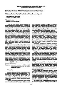
Table 2: cellmeans The graphical presentation of these cellmeans is given in Figure 1 and is obtained by the following command: In [4]:= graphmean[data]

Transactions on Engineering Sciences vol 15, © 1997 WIT Press, www.witpress.com, ISSN 1743-3533

140 Innovation In Mathematics

12

16

20

Figure 1: cellmearis

In Figure 1 a laboratory is given by its number. This graph clearly shows that laboratory 1 has obtained much higher results than all the others. This is confirmed by plotting the h—statistics: In[5]:= graphehstatfdata]

h

i

-2 •

Figure 2: A-values by laboratories In Figure 2, the horizontal lines show the critical values of the h—statistics at a 1% and 5% significance level respectively. The following practice is recommended: if the h—value is less than or equal

Transactions on Engineering Sciences vol 15, © 1997 WIT Press, www.witpress.com, ISSN 1743-3533

Innovation In Mathematics 141 to its 5% critical value, the item tested is accepted as correct; if the A —value is greater than its 5% critical value and less than or equal to its 1%, the item tested is "questionable"; if the /? —value is greater than its 1% critical value, the item tested is called a statistical oW//er ("unsatisfactory''). 3.1.2

Variability of results

As for the averages, the variability of results can be analysed by computing and displaying graphically the intracell standard deviations and the &—statistics. The &—statistics is given in Figure 3 and is obtained by the following command: In[6]:= graphekstat [data]

1.5

0 .5

Figure 3: k-values by laboratories Particularly, this graph shows that the laboratory 7 at the level 4 as well as the laboratory 6 at the level 5 have divergent results. 3.1.3

Numerical tests

Numerical outlier tests can also be made. For example, the Cochran's test is used to judge the intracell standard deviations. In the present case, the Cochran's test statistics takes for each of the 5 level the values:

Transactions on Engineering Sciences vol 15, © 1997 WIT Press, www.witpress.com, ISSN 1743-3533

142 Innovation In Mathematics In [7]:= cochran[data] CW/7/.-^ {0.566474, 0.449912, 0.492417, 0.666703, 0.635778} These values are to be compared to the corresponding critical values at a 1% and 5% significance level respectively: In[8]:= cochcritval[9,2,l] In[9]:= cochcritval[9,2,5] ;= 0.754 /'zr 0.638 These calculations confirm the conclusions obtained by the k— statistics. 3.1.4

Repeatability, reproductibility, general mean

Let's suppose the following scenario: in the light of the preceding tests, the supervisor decides to exclude all the results of laboratory 1 as well as the pair {18.56, 16.58} of results coming from the laboratory 6 at the level 5. With standard Mathematica-commcirids, outlier results can be easily eliminated: In[10]:= pos=Position[Rest[data],{18.56,16.58}]; In[l 1]:= newdata=ReplacePart [Rest [data] , { } ,pos] : The parameters of the new data are computed, for example the repeatability is obtained by: In[12]:= srfnewdata] y.-zz {0.0921615, 0.178903, 0.12691, 0.336796, 0.393474} The other values are given in Table 3. Level j ra, || 6r; SRj 1 3.9406 0.09216 0.17075 2 8.2818 0.17890 0.49768 3 14.1781 0.12691 0.40038 4 15.5881 0.33679 0.57859 20.4121 0.39347 0.63696 5 Table 3: Estimation of raj, 0>j and

From Table 3, it seems that the standard deviations tend to increase with the values of the general mean. Thus, it is possible to establish some form of functional relationship. For example, by plotting the s#-values against

Transactions on Engineering Sciences vol 15, © 1997 WIT Press, www.witpress.com, ISSN 1743-3533

Innovation In Mathematics

143

the m- values a relationship of the form SR — c-m^ seems appropriate. With the Fit-command the parameters c and m are estimated: In[13]:= tR={mhat[newdata],sr[newdata]} //Transpose; In[14]:= regression=(Exp[Fit[Log[tR],{l,x},x]]//Factor)/.x^Log[m] ^;zz 0.0743014 m» ^4325 Figure 4 gives the graphical results of this regression analysis. The final reproductibility standard deviation CTR , as a function of the general mean m should be estimated by

0.6 0.5 0.4 0 .3 0.2 0.1 0

10

15

20

Figure 4: Plot of SRJ against

4

Robust method

Some unsatisfactory features of outlier tests in the ISO-method lead to use statistical robust methods in order to estimate 0>, GR and the general mean m; see [2]. As an illustration of a typical calculation with robust method, let's consider the estimation of the average Tm of a group of measures TI, • • • , #„. The median of these data T = med,{z%} as well as the deviations S- = c- med, {\Xi — T|}, c being a given constant, are calculated successively. We define T® = T and choose for k — 1, 2, • • •

= < Xf,

1.5 • S, if %, if z,1.5.^, if^ -

i < -1.5 •

and then k-l _ r k - l

Transactions on Engineering Sciences vol 15, © 1997 WIT Press, www.witpress.com, ISSN 1743-3533

144 Innovation In Mathematics n^"* being the number of X{ with Xi — T^~*\ < 1.5 • S. In most of the practical cases, the sequence (^*% rapidely converges to the average 7^. Mathematica allows a programmation of such functions in a convenient way. With procedures of this type, estimations of oy, CTR and in have been calculated at each level separately. For example, the following commands give the estimation of the general mean m: In[15]:= data=dat a/ /Transpose; In[16]:= mrobust = Map[globalmean,data] .'^ {3.975, 8.39357, 14.2607, 15.6639, 20.4121}

5

Conclusions

Thus, with the programming flexibility of Mathematica, the statistical analysis of the results of this interlaboratory study can be entirely automatized: on the one hand, the data are read at the beginning in a file and then all necessary results can be obtained by functions of the form function[data\; on the other hand, the graphical capabilities of Mathematica allow the users to see. immediately, the suspicious results. The efficiency of Mathematica in manipulating lists allows the non-specialist users in data analysis or in statistics to carry out interlaboratory experiments in an easy and reliable wav. References [1] ISO 5725-2. Accuracy of measurement methods and results-Part 2. International Organisation for Standardisation, Geneva, Switzerland, 1994. [2] P. LischeT.Statistik und Ringversuche. Schweizerisches Lebensrnittelbuch Kapitel 60 A. Eidg. Drucksachen-und Materialzentrale, Bern, 1989. [3] J. Mandel. yWefVaboroZo?"?/ Te.s/mf/ mW /Zejecfzcm o/ O6erua^ons. Proceedings ISO/REMCO 184. International Organisation for Standardisation, Geneva, Switzerland, 1989.