STABILITY FOR POWER OPERATIONAL AMPLIFIERS

APPLICATION NOTE 19 POWER OPERATIONAL AMPLIFIER M I C R O T E C H N O L O G Y

HTTP://WWW.APEXMICROTECH.COM

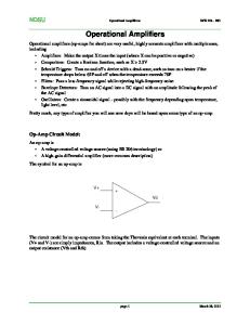
There are two major categories for stability considerations — NonLoop Stability and Loop Stability. Non-Loop Stability covers design areas not related to feedback around the op amp that can cause oscillations in power op amp circuits such as layout, power supply bypassing, and proper grounding. Loop Stability is concerned with using negative feedback around the amplifier and ensuring that the voltage fed back to the amplifier is less than an additional –180 phase shifted from the input voltage. The two key factors to troubleshooting an oscillation problem are: 1) What is the frequency of oscillation? (refer to Figure 1 for definitions of UGBW (Unity Gain Bandwidth) and CLBW (Closed Loop Bandwidth) to be used throughout this text) 2) When does the oscillation occur? 220 200 180

GAIN (dB)

160

RI 100K

100K VOUT

IBIAS IBIAS

VIN CB+ .1µF

RB+ 49.9K

FIGURE 2. RB+

receiving unwanted positive feedback. Calculate your DC errors without the resistor. Some op amps have input bias current cancellation negating the effect of RB+. Some op amps have such low input bias currents that the error is insignificant when compared with the initial input offset voltage. Leave RB+ out, grounding the + input, if possible. If the resistor is required, bypass it with a .1 uF capacitor in parallel with RB+ as shown in Figure 2.

2.3 POWER SUPPLY BYPASSING

140 120

Aol

100 80

CLBW = 10KHz

60

AVCL

40 0 .1

(800) 546-2739

RF

1.0 LOOP STABILITY Vs NON-LOOP STABILITY

20

(800) 546-APEX

UGBW = 1MHz

UNITY GAIN

1

10

100 1K 10K 100K FREQUENCY, f (Hz)

1M

10M

100M

* fosc < UGBW * oscillates unloaded?—no * oscillates with VIN = 0?—may or may not Supply loops are a common source of oscillation problems. Figure 3 shows a case where the load current flows through the supply source resistance and parasitic wiring or trace resistance. This causes a modulated supply voltage to be seen at the power supply pin of the op amp. This modulated signal is then coupled back into a gain stage of the op amp via the compensation capacitor. The compensation

FIGURE 1. DEFINITION OF CLBW & UGBW

The answers to these two questions, along with the sections that follow, should enable you to identify and solve most power op amp stability problems. More importantly, by applying the recommendations in the following sections, you can design power op amp circuits free of oscillation. GAIN STAGE

2.0 NON-LOOP STABILITY 2.1 CASE GROUNDING * fosc < UGBW * oscillates unloaded?—may or may not * oscillates with VIN = 0?—may or may not Ungrounded cases of power op amps can cause oscillations, especially with faster amplifiers. The cases of all APEX amplifiers are electrically isolated to allow for mounting flexibility. Because the case is in close proximity to all the internal nodes of the amplifier, it can act as an antenna. Providing a connection from case to ground forms a Faraday shield around the power op amp’s internal circuitry that prevents noise pickup and cross coupling or positive feedback.

2.2 RB+ BIAS RESISTOR * fosc < UGBW * oscillates unloaded?—may or may not * oscillates with VIN = 0?—may or may not Figure 2 is a standard inverting op amp circuit which includes an input bias current matching resistor on the noninverting input. The purpose of this resistor is to reduce input offset voltage errors due to bias current drops across the equivalent impedance as seen by the inverting and non-inverting input nodes. RB+ can form a high impedance node on the noninverting input which will act as an antenna

POWER STAGE Cc RL

IL Vs

Rs

FIGURE 3. IL MODULATION

capacitor is usually referred to one of the supply lines as an AC ground. Figure 4 shows a second case for supply loop oscillation problems. Power supply lead inductance interacts with a capacitive load forming an oscillatory LC, high Q, tank circuit. Lw +Vs OP AMP CL

FIGURE 4. LC OSCILLATION

APEX MICROTECHNOLOGY CORPORATION • TELEPHONE (520) 690-8600 • FAX (520) 888-3329 • ORDERS (520) 690-8601 • EMAIL [email protected]

Fortunately, both of the above supply line related problems can be eliminated through the use of proper power supply bypass techniques. Each supply pin must be bypassed to common with a “high frequency bypass” .1uF to .22uF ceramic capacitor. These capacitors must be located directly at the power op amp supply pins. In rare cases where power supply line inductance is high, it may be necessary to add 1 to 10 ohms of resistance in series with the high frequency bypass capacitor to dampen the Q of the resultant LC tank circuit. This additional resistor will probably only be necessary when using a wideband amplifier since amplifiers of 5 MHz unity gain bandwidth or less will not respond to the high frequency oscillation caused by line inductance interacting with the high frequency bypass capacitor. Refer to Figure 5.

CL POWER OP AMP

C2 + – +VS

FIGURE 6. EMITTER FOLLOWER WITH C LOAD

C1

< 2"

Rs

OP AMP

Rs –VS

< 2"

C1

Q1

C2 – +

R1

C1 = .1 TO .22 µF, CERAMIC DISC C2 = 10 µF/AMP OUT (PEAK), ELECTROLYTIC Rs = 3 –10Ω (PROVISIONAL– HIGHLY INDUCTIVE P.S. LINES)

L O A D

Q2

R2

FIGURE 5. POWER SUPPLY BYPASSING –Vs

In addition, a “low frequency bypass” capacitor, minimum value of 10uF per Ampere of peak output current, should be added in parallel with the high frequency bypass capacitors from each supply rail to common. Tantalum capacitors should be used when possible due to their low leakage, low ESR and good thermal characteristics. Aluminum Electrolytic capacitors are acceptable for operating temperatures above 0°C. These capacitors should be located within 2" of the power op amp supply pins. Refer to Figure 5.

2.4 MULTIPLE AMPLIFIER BOARDS * fosc < UGBW * oscillates unloaded?—no * oscillates with VIN =0?—yes A prototype circuit is built and bench tested to confirm desired performance. Several channels of the same circuit are used on a printed circuit board layout. Much to the dismay of the design engineer, the amplifier circuits on the printed circuit board oscillate. Cross coupling through the power supply lines can be a major problem on multiple amplifier printed circuit boards. Ground the case of each amplifier and ensure each amplifier has its own power supply bypassing per Section 2.3.

FIGURE 7. COMPOSITE OUTPUT STAGE

power op amps where high current PNP transistors are not readily available. The local feedback in the Q1, Q2 loop will cause output stage oscillations when the output swings negative under reactive loading. RI

RF

VOUT 10 to 100 Ω VIN .1 to 1µF

FIGURE 8. OUTPUT R–C SNUBBER

2.5 OUTPUT STAGE OSCILLATIONS / OUTPUT R-C SNUBBER * fosc > UGBW * oscillates unloaded?—no * oscillates with VIN = 0?— no, only oscillates over a portion of the output cycle Sometimes output stages of power op amps can contain local feedback loops that give rise to oscillations. The first type of output stage instability problem arises from a tendency of emitter followers to appear inductive when looking back into their emitter. This occurs if they are driven from a low impedance source and can create output stage oscillations if capacitance is present on the amplifier’s output. Refer to Figure 6. This type of instability is rare and usually only shows up when driving load capacitances within a limited range of values. The second, more common type of output stage oscillation is due to non-emitter follower output type stages. These stages have heavy local feedback paths. Refer to Figure 7 which is an example of a composite PNP type output stage. This stage is typical of monolithic

Both of these output stage problems can be fixed by using an R-C Snubber on the output of the op amp to ground or the negative supply rail. This is provided the negative supply rail is properly bypassed per Section 2.3. The Snubber network consists of a 10 to 100 ohm resistor in series with a capacitor of .1 to 1 µF (refer to Figure 8). This network lowers the high frequency gain of the output stage preventing unwanted high frequency oscillations.

2.6 GROUND LOOPS * fosc < UGBW * oscillates unloaded?—no * oscillates with VIN = 0?—yes Ground loops come about from load current flowing through parasitic layout resistances and wiring. If the phase of the output signal is in phase with the signal at the node it is fed back to, it will result in positive feedback and oscillation. Although these parasitic resistances (RR in Figure 9) in the load current return line cannot be eliminated, they can be made to appear as a common mode signal to the amplifier.

APEX MICROTECHNOLOGY CORPORATION • 5980 NORTH SHANNON ROAD • TUCSON, ARIZONA 85741 • USA • APPLICATIONS HOTLINE: 1 (800) 546-2739

RI

RF

RF VIN

RI

RR

+ –

Vfb

AOI

VOUT

VOUT β

VIN

VIN

RL RR

Vfb =

VOUT RI

VOUT = VIN Aol – Aol β VOUT

RI + RF

VOUT + Aol β VOUT = Aol

Vfb = β VOUT

RR

RR

“GROUND”

β=

VIN VOUT

RI RI + RF

VIN

IL

=

Aol 1+ Aol β

= 1 β

( FOR: Aol β >> 1) FIGURE 10. BETA (β) – FEEDBACK FACTOR

PROBLEM RI

If Aol β is large, there is a lot of feedback. If Aol β is small, there is not much feedback.

RF

3.2 RATE OF CLOSURE & STABILITY Refer to Figure 11. Aol is the amplifier’s open loop gain curve. 1/β is the closed loop AC small signal gain in which the amplifier is operating. The difference between the Aol curve and the 1/β curve is

VIN “STAR” GROUND POINT

RL 1/β1 100

Aol **

RR

80

SOLUTION

This is done by the use of a “star ground” approach. Refer to Figure 9. The star ground is a point that all grounds are referenced to. It is a common point for load ground, amplifier ground, signal ground and power supply ground.

2.7 PRINTED CIRCUIT BOARD LAYOUT * fosc < UGBW * oscillates unloaded?—may or may not * oscillates with VIN = 0?—no High current output traces routed near input traces can cause oscillations. This is especially true when the output is adjacent to the positive input, giving undesirable positive feedback through capacitive coupling between the adjacent traces. Feedback, input, and bypass components, along with current limit sense resistors, should be located in close proximity to the amplifier. If a printed circuit board has both a high current output trace and a return trace for that high current, then these traces should be routed adjacent to each other (on top of each other on a multi-layer printed circuit board) so they form a twisted pair type of layout. This will help cancel EMI generated outside from feeding back into the amplifier circuit.

3.0 LOOP STABILITY 3.1 BETA β - FEEDBACK FACTOR Control theory is applicable to closing the loop around a power op amp. The block diagram in Figure 10 consists of a circle with an X, which represents a voltage differencing circuit. The rectangle with Aol represents the amplifier open loop gain. The rectangle with the β represents the feedback network. The value of β is defined as the fraction of the output voltage that is fed back to the input; therefore, β can range from 0 (no feedback) to 1 (100% feedback). The term Aol β that appears in the VOUT/VIN equation in Figure 10, has been called “loop gain” because this can be thought of as a signal propagating around the loop that consists of the Aol and β networks.

GAIN (dB)

FIGURE 9. GROUND LOOPS

*

1/β2

60 ** 40 1/β3 *

20

1/β4 0 1

10

100

1K

10K

100K

1M

FREQUENCY, F (Hz) * 20 dB/ DECADE RATE OF CLOSURE ** 40 dB/ DECADE RATE OF CLOSURE

“STABILITY” “MARGINAL STABILITY”

FIGURE 11. RATE OF CLOSURE & STABILITY

the “loop gain”. Loop gain is the amount of signal available to be used as feedback to reduce errors and non-linearities. A first order check for stability is to ensure when loop gain goes to zero, open loop phase shift must be less than 180 degrees where the 1/β curve intersects the Aol curve. Another way of viewing that same criteria is to say at the intersection of the 1/β curve and the Aol curve the difference in the slopes of the two curves, or the RATE OF CLOSURE, is less than or equal to 20 dB per decade. This is a powerful first check for stability. It is, however, not a complete check. For a complete check we will need to check the open loop phase shift of the amplifier throughout its loop gain bandwidth. A 40 dB per decade RATE OF CLOSURE indicates marginal stability with a high probability of destructive oscillations in your circuit. Figure 11 contains several examples of both stable (20 dB per decade) and marginally stable (40 dB per decade) rates of closure.

3.3 EXTERNAL PHASE COMPENSATION External phase compensation is often available on an op amp as a method of tailoring the op amp’s performance for a given application. The lower the value of compensation capacitor used the higher the slew rate of the op amp. This is due to fixed current sources inside the front end stages of the op amp. Since current is fixed, we see from the relationship of I = CdV/dt that a lower value of capacitance will yield a faster voltage slew rate.

APEX MICROTECHNOLOGY CORPORATION • TELEPHONE (520) 690-8600 • FAX (520) 888-3329 • ORDERS (520) 690-8601 • EMAIL [email protected]

CF

RF RI

1

STABLE FOR ANY Cc

2

STABLE FOR ANY Cc = 0pF

RF

Aol

RI

1/β AVCL

VIN

Vfb

VOUT

Cc VNOISE

SMALL SIGNAL RESPONSE

1 2π RF CF RI + RF fz = 2π RI RF CF

fp =

120 fp1

Cc = 33pF

100

Cc = 0pF

Aol

80 80

fp2

60

GAIN (dB)

OPEN LOOP GAIN Aol (dB)

100

1 40 2

60

Aolβ 40 40 dB DECADE fcl

20 20

0 1

10

100

1K

10K

.1M

1M

10M

FREQUENCY, F (Hz) FIGURE 12. EXTERNAL PHASE COMPENSATION

1β 0 1

fp 10

100

1K fz

10K

100K

1M

FREQUENCY, F (Hz) FIGURE 13. STABILITY– RATE OF CLOSURE

However, the advantage of a faster slew rate has to be weighed against AC small signal stability. In Figure 12 we see the Aol curve for an op amp with external phase compensation. If we use no compensation capacitor, the Aol curve changes from a single pole response with Cc = 33pF, to a two pole response with Cc = 0pF. Curve 1 illustrates that for 1/β of 40 dB the op amp is stable for any value of external compensation capacitor (20 dB/decade rate of closure for either Aol curve, Cc = 33pF or Cc = 0pF). Notice that 1/β curve continues on past the intersection of the Aol curve. At the intersection of 1/β and Aol, the AVCL closed loop gain curve, or VOUT/VIN gain begins to roll off and follow the Aol curve. This is because there is no loop gain left to keep the closed loop gain flat at higher frequencies. Curve 2 illustrates that for 1/β of 20 dB and Cc = 0pF, there is a 40 dB/decade rate of closure or marginal stability. To have stability with Cc = 0pF minimum gain must be set at 40dB. This requires a designer to not only look at slew rate advantages of decompensating the op amp, but also at the gain necessary for stability and the resultant small signal bandwidth.

3.4 STABILITY - RATE OF CLOSURE Figure 13 shows a typical single pole op amp configuration in the inverting gain configuration. Notice the additional VNOISE voltage source shown at the +input of the op amp. This is shown to aid in conceptually viewing the 1/β plot. An inverting amplifier with its +input grounded, will always have potential for a noise source to be present on the +input . Therefore, when one computes the 1/β plot, the amplifier will appear to run in a gain of 1 + RF/RI for small signal AC. The VOUT/VIN relationship will still be –RF/RI. This is also why an amplifier can never run at a gain of less than one for small signal AC stability considerations. The plot in Figure 13 shows the open loop poles from the amplifier’s Aol curve, as well as the poles and zeroes from the 1/β curve. The locations of fp and fz are important to note as we will see that poles in the 1/β plot will become zeroes and zeroes in the 1/β plot will become poles in the open loop stability check. Notice that at fcl the RATE OF CLOSURE is 40 dB per decade indicating a marginal stability condition. The difference between the Aol curve and 1/β curve is labelled Aol β which is also known as loop gain.

3.5 STABILITY - OPEN LOOP Stability checks are easily performed by breaking the feedback path around the amplifier and plotting the open loop magnitude and phase response. Refer to Figure 14. This open loop stability check has the first order criteria that the slope of the magnitude plot as it crosses 0 dB must be 20 dB per decade for guaranteed stability. The 20 dB per decade is to ensure the open loop phase does not dip to –180 degrees before the amplifier circuit runs out of loop gain. If the phase did reach -180, the output voltage would now be fed back in phase with the input voltage (-180 degrees phase shift from negative feedback plus -180 degrees phase shift from feedback network components would yield -360 degrees phase shift). This condition would continue to feed upon itself causing the amplifier circuit to break into uncontrollable oscillations. Notice in Figure 14 this open loop plot is really a plot of Aol β. The slope of the open loop curve at fcl is 40 dB per decade indicating a marginally stable circuit. As shown, the zero from the 1/β plot in Figure 13 became a pole in the open loop plot in Figure 14 and likewise the pole from the 1/β plot in Figure 13 became a zero in the open loop plot of Figure 14. We will use this knowledge to plot the open loop phase plot to check for stability. This plot of the open loop phase will provide a complete stability check for the amplifier circuit. All the information we need will be available from the 1/β curve and the Aol curve.

4.0 STABILITY & THE INPUT POLE / INPUT & FEEDBACK IMPEDANCE * fosc < CLBW * oscillates unloaded?—yes * oscillates with VIN = 0?—yes All op amps have some input capacitance, typically 6-10 pF. Printed circuit layout and component leads can introduce additional input stray capacitances. When high values of feedback and input resistors are used, this input capacitance will contribute an additional pole to the loop gain response (a zero in the 1/β plot, a pole in the open loop phase check for stability, or a pole in the Aol β, loop gain, plot).

APEX MICROTECHNOLOGY CORPORATION • 5980 NORTH SHANNON ROAD • TUCSON, ARIZONA 85741 • USA • APPLICATIONS HOTLINE: 1 (800) 546-2739

CF

We will refer to Figure 15 for a detailed look at the input pole and stability. Remember, our first order criteria for stability is a Rate Of Closure of 20dB per decade or less. Curve 1 is the op amp’s Aol plot. Curve 5 shows the effect of input capacitance with no CF feedback capacitor. We see the rate of closure is 40 dB per decade and marginal stability exists. With just CI present, as frequency increases, the impedance from the -input of the op amp decreases, thereby causing the 1/β plot to increase (remember XCI = 1/2πfCI). If we now add some small value of CF as in Curve 2 we see the 1/β plot flatten out to intersect the Aol at a rate of closure 20 dB per decade implying stability. If we further increase CF, as in Curve 3, such that both breakpoints are the same frequency, we will have ZF/ZI constant over frequency and the 1/β plot will be flat with frequency. This yields the ever-stable 20 dB per decade rate of closure. If we then continue to increase CF as in Curve 4, we will see CFdominate as frequency increases and the net result is a low pass filter frequency roll-off. For this case the op amp must be unity gain stable, since the op amp operates at a gain of one for frequencies above 10KHz. Often you will see CF recommended to be used to decrease overshoot and improve settling time for a transient input into a given op amp circuit. In the AC small signal domain, we are merely optimizing the circuit for stability. Minimize values of feedback and input resistor values. This will reduce the effect of the input pole as well as help reduce DC errors by keeping voltage drops due to bias currents low. A summing node of an op amp can pick up unwanted AC signals and amplify them if that node is high impedance. Keeping the feedback and input resistance values low will reduce the impedance at the summing nodes and minimize stray signal pick up. Practical values for feedback and input resistance values are from 100 ohms to 1 megaohm.

RF VOUT VIN

1 2π RF CF RI + RF fp = 2π RI RF CF fz =

100

fp1

80 GAIN (dB)

fp

(fp2 + fz)

60

Aolβ 40 40 dB DECADE

20

fcl 0

1

10

100 1K 10K FREQUENCY, F (Hz)

100K

1M

5.0 LOOP STABILITY EXAMPLES 5.1 VOLTAGE TO CURRENT CONVERSION— FLOATING LOAD

FIGURE 14. STABILITY– OPEN LOOP CF

RF

RI

CI

1

Aol

2

CI / CF > RF / RI

3

CI / CF = RF / RI

4

CF >> CI

5

RF / X CI

* fosc < CLBW * oscillates unloaded ? — yes * oscillates with VIN = 0 ? — yes Figure 16 illustrates a common voltage to current conversion circuit. The input command voltage of +/-10V is scaled to control -/+1.67A of output current through the load. +28V

CI / CF =

RCL + .301Ω

X CF / X CI

PA07

RI

120 VIN ±10V

100

RL 9Ω

RCL–

4.99K

.301Ω –28V

FB#2 RF

Rd Cf

LL 159mH

FB#1

1

80

1K

GAIN (dB)

IOUT 1.67A

±

RI

60 2 40

FIRST GUESS FINAL VALUES

5

Rs 1.2Ω

VRs

Rd Cf 825K 820pF 82.5K .068µF

FIGURE 16. V-I CIRCUIT AND STABILITY

20 3 0 4 –20 1

10

100

1K

10K

100K

FREQUENCY, F (Hz) FIGURE 15. THE INPUT POLE

1M

10M

This V-I (Voltage to Current) topology is a floating load drive. Neither end of the load, series RL and LL, is connected to ground. The easiest way to view the voltage feedback for load current control in this circuit is to look at the point of feedback which is the top of Rs. The voltage gain VRs/Vin is simply -RF/RI which translates to (–1K/ 4.99K = -.2004). The Iout/Vin relationship is then VRs/Rs or Iout = - Vin (RF/RI)/Rs which for this circuit is (Iout = -.167 Vin). We will use our knowledge of 1/β, Rate of Closure, and open loop stability phase plots, to design this V-I circuit for stable operation. There are two voltage feedback paths around the amplifier, FB#1 and FB#2. We will analyze FB#1 first and then see why FB#2 is necessary for guaranteed stability.

APEX MICROTECHNOLOGY CORPORATION • TELEPHONE (520) 690-8600 • FAX (520) 888-3329 • ORDERS (520) 690-8601 • EMAIL [email protected]

STABILITY SOLUTION FOR V-I CIRCUIT

220 200

STEP 1: On Figure 17 plot the op amp’s Aol curve as given by the manufacturer.

180 160

GAIN (dB)

220 200 180 GAIN (dB)

160

100

PA07 Aol fp1

100

FB#1 fp FB#2

fz1

60

PA07 Aol

fp1

FB#1

40 20

80

1/β 1

0 .1

60 40

fp2 1

10

100 1K 10K 100K FREQUENCY, F (Hz)

1M

fp2

10

100

1K

10K

100K

1M

10M

250 FREQUENCY, F (Hz)

fz

20 0 .1

120 80

140 120

140

10M

100M

fp3

3p

3p

100M fp3

FIGURE 19. FIRST GUESS MAGNITUDE PLOT FOR STABILITY

and PA07 Aol curve to plot the open loop phase plot. Remember the following rules when plotting open loop phase plots for stability checks.

FIGURE 17. Aol AND FB # 1 – MAGNITUDE PLOT FOR STABILITY

RULES FOR PLOTTING OPEN LOOP PHASE PLOTS

STEP 2: On Figure 17 plot FB#1. Refer to Figure 18 for calculation of FB#1. At DC, LL is a short and so β is a voltage divider through resistors as shown in Figure 18. As we go to higher frequencies, the reactance of LL will increase (XL = 2πfL). This will increase the net load impedance which will cause β to decrease and 1/β to increase as frequency increases. Since we are working with a single reactive element the increase of that gain will be 20 dB per decade. Figure 18 details the breakpoint fz where this increase begins. We see that at the intersection of FB#1 and the PA07 Aol curves the rate of closure is 40 dB per decade indicating marginal stability.

1)

VOUT (1)

Vfb (.098) RI 4.99K

RF 1K

RL 9Ω

DC β ( LL = 0, Cf = ∞ )

FB #1 β =

Vfb VOUT

β = .098 Rs 1.2Ω

fz =

1/β = 10.2

Rs + RL 2π

LL

=

1.2Ω + 9Ω 2π 159mH

20dB = 10.2Hz

FIGURE 18. FEEDBACK NO.1 (FB #1)

STEP 3: Refer to Figure 19 which repeats PA07 Aol and FB#1. We will add FB #2 to force the high frequency part of the 1/β curve to flatten out and intersect the PA07 Aol curve at 20 dB per decade. FB #2 will dominate at frequencies above 1 KHz. Although our V-I circuit has two feedback paths, the op amp will follow whichever feedback path is dominant. This means the larger β is, the more voltage is fed back from the output to the -input as negative feedback (Remember β = Vfb/VOUT). With a larger β, 1/β will become smaller; therefore, the dominant feedback path out of FB#1 and FB#2 will be the lowest gain path. Plot a desired feedback path for FB#2. At high frequencies, FB#2 will be a flat line since Cf will be a short leaving a pure resistive divider for β. At DC, FB#2 will be infinite since Cf is an open. This will be limited by the PA07 Aol curve. Since we only have one reactive element in FB#2, we will have a 20 dB per decade slope from low to high frequency. Set fz1 one half to one decade below the intersection of FB#1 and FB#2. This “Decade” rule of thumb ensures that as component values and Aol curves vary we will not get into stability trouble—more about this later. STEP 4: In Figure 19 the long-dashed line represents the 1/β feedback path that the PA07 operates in for small signal AC. According to our first order check for stability we see a 20 dB per decade rate of closure indicating a stable design. But let’s do our complete stability check by using the 1/β curve

Poles in 1/β plot become zeroes in the open loop stability check. 2) Zeroes in 1/β plot become poles in the open loop stability check. 3) Poles and zeroes in the Aol curve of the op amp remain respectively poles and zeroes in the open loop stability check since the op amp Aol curve is an open loop curve already. 4) Phase for poles is represented by a -45 degree phase shift at the frequency of the pole with a -45 degree per decade slope, extending this line with 0 degree and -90 degree horizontal lines. 5) Phase for zeroes is represented by a +45 degree phase shift at the frequency of the zero with a +45 degree per decade slope, extending this line with 0 degree and +90 degree horizontal lines. Figure 20 is the resultant open loop phase plot using the information from Figure 19. After plotting individual open loop poles and zeroes, and drawing the appropriate slopes, we graphically add the slopes to yield a resultant open loop phase as shown in Figure 20. Notice fp3 in Figure 20 is a triple pole. It is easier to plot this as shown in Figure 20 as three poles “on top” of each other. This makes it easier to add graphically for a resultant open loop phase plot. As shown in Figure 20, our open loop phase dips to -180 at 100Hz. Our first attempt at compensation was not successful since we desire at least 45 degrees of phase margin (open loop phase should not dip to less than -135 degrees). STEP 5: We need to revisit FB#2 to make this V-I circuit stable. Figure 21 shows a new FB#2 and the resultant 1/β plot. Before we look at the open loop phase plot, let’s discuss Figure 21. We see that in the PA07 Aol curve there is a pole at fp1, 10Hz, which will be a pole in our open loop phase plot. We also see a zero at fz, 10Hz, in the 1/β plot, which will become a pole in our open loop phase plot. Now we have two poles at 10Hz in our open loop phase plot. To keep the open loop phase from reaching -180, we must add a zero at 100Hz to get 45 degrees of phase margin. Poles and zeroes a decade beyond fcl, the intersection of 1/β and PA07 Aol, are of no concern for stability since at fcl the loop gain is zero. The reason we must look a decade beyond fcl on the magnitude plot is that poles and zeroes have an effect on phase plus or minus a decade away from their physical location on the magnitude plot. Viewing the magnitude plot in this way can help us save iterative steps in compensating to guarantee good stability. Refer to Figure 22 (see second page following this one) for final open loop phase plot stability. Once the open loop phase plot verifies stability, it is time to compute final values for FB#2 components Rd and Cf. Figure 23 details these

APEX MICROTECHNOLOGY CORPORATION • 5980 NORTH SHANNON ROAD • TUCSON, ARIZONA 85741 • USA • APPLICATIONS HOTLINE: 1 (800) 546-2739

+180 +135

fp

+90 +45 fp1

0 –45

fp3

fz

fp2

–90 –135 –180 .1

1

10

100

1K

10K

.1

1

10

100

1K

.1

1

10

100

1K 10K FREQUENCY, F (Hz)

100K

1M

10M

100M

100K

1M

10M

100M

100K

1M

10M

100M

PHASE SHIFT (degrees)

+180 +135 +90 +45 0 –45 –90 –135

φ MARGIN = 0 DEGREES

–180

10K

+180 +135 +90 +45 0 –45 –90 –135 –180

FIGURE 20. FIRST GUESS OPEN LOOP PHASE PLOT FOR STABILITY

5.2 CAPACITIVE LOADING & STABILITY * fosc < CLBW * oscillates unloaded?—no * oscillates with VIN = 0?—yes

220 200 180 160

GAIN (dB)

calculations. Notice in Figure 23 that to work with β it is easiest to set Vout to 1 which then allows us to easily use voltage dividers and currents to calculate values for Rd. Cf is computed as given by the formula in Figure 23. OPEN LOOP PHASE PLOTS FOR STABILITY — FINAL NOTE: This hand plotting technique is a linear graphical method. Actual magnitude plots run on such analog circuit simulations as SPICE will be 3 dB different and actual phase plots will be 6 degrees different.

140 120

PA07 Aol fp1

100 80 60

fz1

40 0 .1

1/β 1

5.2.1 CAPACITIVE LOADING - GENERAL

5.2.2 CABLE AND CAPACITIVE LOADING Beware of coaxial cables which can appear capacitive. A coaxial cable appears capacitive, instead of its characteristic impedance, resistive, if the length of the cable is less than one-fortieth of the wavelength in the cable at the frequency of interest, f. This length, l, is given by: l≤

1 Kc meters 40 f

fp FB#2

fz

20

Refer to Figure 24 (see second page follwong this one) for discussion of power op amps and capacitive loading. The output impedance of a power op amp, Ro, can interact with capacitive loads and form an additional high frequency pole in the op amp’s Aol curve. This modified Aol curve is what we must look at for stability checks. In Figure 24, we see a modified Aol curve whose slope changes from 20 dB per decade to 40 dB per decade at 10 kHz. Note that the rate of closure for this circuit is 40 dB per decade indicating marginal stability.

FB#1

10 100 1K 31.6 250

10K fcl

100K

1M

10M

100M

fp2

FREQUENCY, F (Hz)

3p

fp3

FIGURE 21. FINAL VALUE MAGNITUDE PLOT FOR STABILITY

where K is a propagation constant that is sometimes called the velocity factor (0.66 for coaxial cable) and c is the velocity of light (3.00 X108 m/s). EXAMPLE: If f = 10KHz: l≤

1 (0.66) (3x108) = 495 meters (1624 feet) 40 104

Cables less than 495 meters will appear capacitive for 10 kHz signals at the rate of 95 pF/meter (29 pF/foot) for RG-58A/U, a commonly used coaxial cable.

APEX MICROTECHNOLOGY CORPORATION • TELEPHONE (520) 690-8600 • FAX (520) 888-3329 • ORDERS (520) 690-8601 • EMAIL [email protected]

+180 +135 +90 +45 0

fz

–45

fp2

fp3

fp1

–90 –135 –180 .1

1

10

100

1K

10K

100K

1M

10M

100M

10M

100M

10M

100M

PHASE SHIFT (degrees)

+180 +135 +90

fp

+45 0

ADD ZERO FOR 45° φ MARGIN

–45 –90 –135 –180 .1

1

10

100

1K

10K

100K

1K FREQUENCY, F (Hz)

10K fcl

100K

1M

+180 +135 +90 +45 0 –45 –90 –135

φ MARGIN = 45°

–180 .1

1

10

100

1M

FIGURE 22. FINAL VALUE OPEN LOOP PHASE PLOT FOR STABILITY

VOUT (1) Vfb (.01)

Rd

RI 4.99K

RF 1K

FB #2 Ifb

HI – fβ ( CF = 0, LL= ∞ )

1/β = 40dB = 100 RI // RF ≈ 833Ω

β = .01

Ifb = Vfb / (RI // RF) = .01/833Ω = .12mA

Rs 1.2Ω

RT = VOUT / Ifb = 1/.012mA = 83.3K Rd ≈ RT – (RI // RF) = 83.3K – 833 ≈ 82.5K USE 82.5K fz1 =

1 2π Rd Cf

= 31.6Hz

Cf = .068µF

GAIN (dB)

Aol FB #2

NOTE: AVOID DOUBLE POLE IN 1/β PLOT AT FR –– COMPLEX POLES IN FB #1 OPEN LOOP STABILITY –– –180° PHASE SHIFT AT FR.

1/β

FR FREQUENCY, F(Hz) FIGURE 23. FEEDBACK NO. 2 (FB #2) FINAL VALUE CALCULATIONS

5.2.3 AMPLIFIER OUTPUT IMPEDANCE, Ro AND CAPACITIVE LOADING In the design of power amp circuits, the need often arises for a power amp model with specified output impedance. Most often, this requirement revolves around the need to accurately predict the phase performance of power amp circuits. Output impedance of any op amp is modified by the feedback network present around the device. In voltage source type circuits, the effect of the network is to reduce the output impedance by a factor equal to the ratio of open loop gain to closed loop gain. In power amps, the net result is an effective output impedance of milliohm levels at frequencies below 1kHz. Wiring and interconnections often create larger impedances than the output impedance of the closed loop power amp. Therefore, output impedance will play a minor role in the phase performance at low frequencies. At high frequencies, reactive load considerations are already addressed by capacitive load specifications given on many power amplifiers. Within the bandwidth of the amplifier the output impedance of most APEX power op amps appears predominantly resistive. As an output stage drives higher currents, its output impedance changes when compared to the low current or unloaded output impedance. In general, this impedance reduces as current is driven through the output stage. When compensating circuits with capacitive loading we will use the low current or unloaded output impedance for Ro. This will be the highest value of Ro causing the lowest frequency additional pole which modifies an amplifier’s Aol curve when driving a capacitive load. Many designs in the past have verified that compensating for this condition will give the best stability for all conditions when driving capacitive loads.

APEX MICROTECHNOLOGY CORPORATION • 5980 NORTH SHANNON ROAD • TUCSON, ARIZONA 85741 • USA • APPLICATIONS HOTLINE: 1 (800) 546-2739

The following is a list of output impedances for APEX power op amps and boosters. OP AMP OR BOOSTER

RF

OUTPUT IMPEDANCE RI

5.2.4 COMPENSATING CAPACITIVE LOADS There are two main ways to compensate for capacitive loads or two pole Aol curves. The “Feedback Zero” and “Noise Gain” or “Input RC Network” compensation techniques for capacitive loads will both be discussed. The “Feedback Zero” technique uses a pole in the 1/β plot (a zero in the open loop phase check for stability or a zero in the Aol β, loop gain, plot) to compensate for the additional pole due to capacitive loading in the amplifier’s modified Aol curve. Refer to Figure 25. Note that in Curve 1 there is both a pole and zero in this 1/β plot. The pole is due to the interaction of Rf and Cf. The zero can be found by graphically extending the 1/β plot to zero dB. Remember from previous discussion that an op amp cannot operate at a gain of less than 1 for small signal AC. The “Noise Gain” compensation technique raises the small signal AC gain of the amplifier to run at a gain that is high enough to ignore the additional high frequency pole in the Aol curve due to capacitive loading. Refer to Figure 25. Curve 2 shows the 1/β plot for noise gain compensation. Notice in Figure 25 that both Curve 1 and Curve 2 yield a 20 dB per decade rate of closure implying stability; whereas, with just resistive feedback at the given gains the circuits would be unstable with a 40 dB per decade rate of closure.

5.2.4.1 FEEDBACK ZERO COMPENSATION Figure 26 illustrates a circuit utilizing Feedback Zero Compensation for stability when driving a capacitive load. Figure 27 is our magnitude plot to work with for stability. The following procedure will ensure a logical approach to optimize stability:

Ro CL

UNITY GAIN STABLE AMPLIFIER BUT: UNSTABLE 40 dB/DECADE WITH CL

SMALL SIGNAL RESPONSE

120

100 OPEN LOOP GAIN AOL (dB)

PA01 ................................... 2.5-8.0 ohms PA02 ................................... 10-15 ohms PA03 ................................... 25 ohms PA04 ................................... 2.0 ohms PA05 ................................... 5 ohms PA07 ................................... 1.5-3.0 ohms PA08 ................................... 1.5K-1.9K ohms PA09 ................................... 15-19 ohms PA10 ................................... 2.5-8.0 ohms PA12 ................................... 2.5-8.0 ohms PA19 ................................... 30-40 ohms PA21, 25, 26 ....................... 10 ohms PA41, PA42, PA43 ............. 150 ohms PA45 ................................... 150 ohms PA51 ................................... 1.5-1.8 ohms PA61 ................................... 1.5-1.8 ohms PA73 ................................... 1.5-1.8 ohms PA81J ................................. 1.4K-1.8K ohms PA82J ................................. 1.4K-1.8K ohms PA83 ................................... 1.4K-1.8K ohms PA84 ................................... 1.4K-1.8K ohms PA87 ................................... 50 ohms PA85 ................................... 50 ohms PA88 ................................... 100 ohms PA89 ................................... 100 ohms PB50 ................................... 35 ohms PB58 ................................... 35 ohms

80

60

40 UNSTABLE

STABLE

20

0 –100 1

10

100 1K 10K .1M FREQUENCY, F (Hz)

1M

10M

Aol

1/β

Aol WITH CL

AVCL

FIGURE 24. CAPACITIVE LOADING

STEP 1: Modify the PA88 Aol due to CL. Here we use the output impedance number for the PA88 of Ro = 100 ohms. fp2 =

1 1 = = 10 kHz 2π Ro CL 2π 100 159nF

The higher frequency poles of the unmodified PA88 Aol must be added into the modified Aol as shown in Figure 26. STEP 2: Calculate DC β for circuit. DC β = RI/(RF + RI) = 10K/(316K+10K) = .030674846 DC 1/β = 20 Log (1/.030674846) = 30.26 dB

STEP 3: Plot DC 1/β. Add pole in 1/β plot to compensate for fp2. Ensure fp5 is one-half to one decade away from fcl such that if the modified Aol plot in the real world moves to the left towards lower frequency we will not be back at a 40 dB per decade rate of closure. Note in Figure 27 that the 1/β plot has fp5 and fz1. The feedback network continues to feed back output voltage beyond fcl until we reach 0 dB. Then the 1/ β plot flattens out at 0 dB. It is important to include fz1 since it will be a pole in our open loop phase check and will affect phase at frequencies lower than fcl. At fcl loop gain is zero

APEX MICROTECHNOLOGY CORPORATION • TELEPHONE (520) 690-8600 • FAX (520) 888-3329 • ORDERS (520) 690-8601 • EMAIL [email protected]

CF

RF CF 47pF

316K

RF RI

+225V

RCL

RI

6.5Ω

CL

10K

PA88

VIN

CL 159nF

1

1/β

FEEDBACK ZERO COMPENSATION RI

– 225V

Cc 3.3pF

RF

FIGURE 26. FEEDBACK ZERO COMPENSATION FOR CL Rn

220 200

Cn

180

CL

160 GAIN (dB)

2

1/β

NOISE GAIN COMPENSATION

SMALL SIGNAL RESPONSE

120

PA88 w/Cc = 3.3pF

100

fp1

80

120

fp2

60

1/β

40

Aol

fp5

fcl fz1

20

100 OPEN LOOP GAIN AOL (dB)

140

VO / VIN

0 .1

1

10

80

dp 100 1K 10K 100K FREQUENCY, F (Hz)

1M

MODIFIED Aol : RO = 100Ω , CL = 159nF 60

100M

fp4 fdp3

FIGURE 27. FEEDBACK ZERO COMPENSATION FOR CL MAGNITUDE PLOT FOR STABILITY

40 1

2

20

0

–100 1

10M

10

100

1K

w/CL

w/o CL

.1M

1M

10K

10M

FREQUENCY, F (Hz) FIGURE 25. CAPACITIVE LOAD COMPENSATION

and beyond fcl we are not concerned with phase shift to guarantee stability. Note that the VO/VIN plot follows the 1/β plot until at which point there is no loop gain and VO/VIN will follow the Aol curve on down in gain. STEP 4: Plot open loop phase as in Figure 28. We see we have 67 degrees of phase margin and therefore guaranteed stability. STEP 5: Once you have chosen CF to get the fp5 you want you automatically set fz1. fz1 can be gotten graphically from the 1/β plot. For those of you who want exact breakpoints, here are the formulae for the 1/β plot in Figure 27. fp5 = fz1 =

1 2π RF CF RI + RF 2π CF RI RF

5.2.4.2 NOISE GAIN COMPENSATION Figure 29 illustrates how Noise Gain compensation works. One way to view noise gain circuits is to treat the amplifier as a summing amplifier. There are two input signals into this inverting summing

amplifier. One is VIN and the other is a noise source summed in via ground through the series combination of Rn and Cn. Since this is a summing amplifier, VO/VIN will be unaffected if we sum zero into the RnCn network. However, in the small signal AC domain, we will be changing the 1/β plot of the feedback as when Cn becomes a short and if Rn RIN

FIGURE 41. DYNAMIC STABILITY TEST

APEX MICROTECHNOLOGY CORPORATION • TELEPHONE (520) 690-8600 • FAX (520) 888-3329 • ORDERS (520) 690-8601 • EMAIL [email protected]

CONDITION AND PROBABLE CAUSE TABLE Oscillates unloaded? Oscillates with VIN = 0? Loop Check† fixes oscillation? Oscillation Probable Cause(s) Frequency (in order of probability) N Y N C, D fosc ≤ UGBW fosc ≤ CLBW

Y

Y

Y

fosc ≤ UGBW

–

–

N

G, A, M, B

fosc ≤ CLBW

N

Y

Y

D J, C

10.0 APPENDIX This appendix contains some handy tools for plotting magnitude and phase plots for stability analyses. The “Log Scaling Technique” covers an easy way to read exact frequency locations of poles and zeroes from magnitude plots for stability. Included, as well, are blank magnitude and phase plots for copying and using to plot phase and magnitude plots for stability. One final tip. Once a magnitude plot has been plotted containing the Aol curve and 1/β, it is easy to translate the poles and zeroes to an open loop phase plot for stability. Simply use a light table (ours is very basic — a piece of plexiglass that fits over a 60W incandescent desk light !) to trace the locations of poles and zeroes. Remember poles and zeroes in the Aol curve are poles and zeroes in the open loop phase check for stability. But poles in the 1/β plot become zeroes, and zeroes in the 1/ β plot become poles in the open loop phase check for stability.

K, E, F, J

fosc ≤ UGBW

Y

Y

N*

fosc ≤ CLBW

Y

Y

N

L, C

fosc > UGBW

N

Y

N

B, A

fosc > UGBW

N

N**

N

A, B, I, H

CLBW = Closed Loop Bandwidth UGBW = Unity Gain Bandwidth † See Figure 42A for loop check circuit. — Indeterminate; may or may not make a difference. *Loop check (Figure 42A) will stop oscillation if Rn