JAMES A. BAKER III INSTITUTE FOR PUBLIC POLICY RICE UNIVERSITY

SPECULATION, FUNDAMENTALS, AND THE PRICE OF CRUDE OIL BY

KENNETH B. MEDLOCK III JAMES A BAKER III AND SUSAN G BAKER FELLOW IN ENERGY AND RESOURCE ECONOMICS, AND SENIOR DIRECTOR, CENTER FOR ENERGY STUDIES, JAMES A BAKER III INSTITUTE FOR PUBLIC POLICY, RICE UNIVERSITY

AUGUST 2013

THIS PAPER WAS WRITTEN BY A RESEARCHER WHO PARTICIPATED IN A BAKER INSTITUTE RESEARCH PROJECT. WHEREVER FEASIBLE, PAPERS ARE REVIEWED BY OUTSIDE EXPERTS BEFORE THEY ARE RELEASED. HOWEVER, THE RESEARCH AND VIEWS EXPRESSED IN THIS PAPER ARE THOSE OF THE INDIVIDUAL RESEARCHER, AND DO NOT NECESSARILY REPRESENT THE VIEWS OF THE JAMES A. BAKER III INSTITUTE FOR PUBLIC POLICY.

© 2013 BY THE JAMES A. BAKER III INSTITUTE FOR PUBLIC POLICY OF RICE UNIVERSITY THIS MATERIAL MAY BE QUOTED OR REPRODUCED WITHOUT PRIOR PERMISSION, PROVIDED APPROPRIATE CREDIT IS GIVEN TO THE AUTHOR AND THE JAMES A. BAKER III INSTITUTE FOR PUBLIC POLICY.

Speculation, Fundamentals, and the Price of Crude Oil Abstract The causes and consequences of rising oil price over the past decade has been the subject of much debate. The role of speculation in financial markets has come increasingly under the microscope with many economists arguing that in commodity markets, such as oil, inventory adjustment should prevent speculative pressures from unduly influencing price. However, if demand and supply are relatively inelastic (not very price responsive) in the short run, then inventory adjustment can be slow to occur. In turn, the theory presented herein suggests that speculative activity can exacerbate price movements that are hinged on underlying market fundamentals. In other words, when constraints are present, inventory adjustment can be sluggish, which will reinforce the speculative notion that markets are becoming tighter. This will continue until something happens to unhinge that expectation, such as inventory build or economic collapse. Otherwise, speculation cannot exert an influence on price. This paper investigates whether speculative pressures can exert an influence on the price of storable commodities, such as crude oil and natural gas.

3

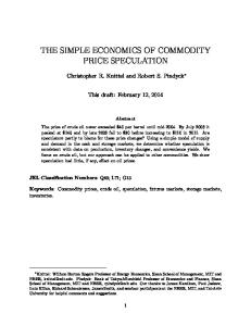
Speculation, Fundamentals, and the Price of Crude Oil I. Introduction The price of crude oil has been the subject of intense scrutiny for many years. The price oil has been linked broadly to macroeconomic dislocations,1 which raises concerns over energy security. Crude oil price is, indirectly, among the most public commodity price. Specifically, the price of gasoline and diesel – a derivative of crude oil price – is openly posted at fueling stations on street corners, making it the most public price of any energy commodity thereby placing oil immediately in the minds of consumers everywhere. These factors taken together have made the price of oil a highly politicized variable, with much deliberation over the causes and consequences of increasing oil prices. Figure 1. Refiner Acquisition Cost of Crude (Monthly, Jan 1974 – Mar 2013)

Source: US Energy Information Administration

1

Whether or not there is a causal relationship is still a subject of intense discussion in the academic literature, but the correlation between oil price and short term economic growth is widely recognized. 2 See, for example, Jaffe and Soligo (2007). 3 See Hubbert (1956). 4 Generally, a logistics curve is fit to historical data to ascertain the point at which a basin’s peak production will occur. Thus, it is conditional on observed history, but does not take explicit account of commercial drivers of

4

Speculation, Fundamentals, and the Price of Crude Oil The last ten years has seen the real oil price rise to levels not witnessed in three decades (see Figure 1). This has triggered a considerable amount of discussion and analysis as to what is behind such dramatic price movements. The discussions about the contributing factors have varied, but have generally centered on: (i) a lack of investment by “big” oil, (ii) concerns about an impending peak in global oil production, (iii)the “graying” of the oil industry, shortages of specialized labor and services, and rising costs of production, (iv) the role of national oil companies in balancing the global oil market and what governs their production decisions, (v) rapid demand growth in developing Asia and China in particular, (vi) the declining value of the US dollar, and (vii)

speculation.

Indeed, the last of these points – speculation – has perhaps triggered the greatest amount of discussion in the last 5 years. Each of the above listed possible price drivers – (i) through (vii) – either influences or is influenced by expectations about future market outcomes. An indication of expectations regarding oil price can be gleaned from historical price forecasts of the US Energy Information Administration (EIA). Figure 2 indicates the EIA’s 10 year projections for the price of oil from 1979 through 2013. Specifically, the thick black line is the actual price of oil and the projections for each year are depicted in the colored lines which launch from the actual price. During the 1990s and early 2000s, the projections tend to all converge on a price of $30 per barrel. Not until 2005 do we begin to see projections of $50, but even then the trajectory of expected prices is relatively flat, until we get to 2008. Since 2008, we see projections for oil price that tend to be increasing well into the forecast horizon. Note that the pattern so described is similar to what we see in the late 1970s and early 1980s. Specifically, the trajectory of price projections does not being to change until several years after the actual price has been moving in a particular direction. This can be indicating that expectations are adaptive, or dependent on recent history.

5

Speculation, Fundamentals, and the Price of Crude Oil Indeed, closer examination of Figure 2 reveals that the spread between the current price and the ten year projection for each year is very high from 1979 through 1985 and from 2008 through 2013. This indicates that factors in these years were contributing to an expectation that price would rise for the foreseeable future. In all other years, the spread between the forecast and current price is relatively small. Figure 2. 10-Year Nominal Oil Price Projections (Annual, 1979-2013)

Source: US Energy Information Administration

This raises the issue of whether or not oil prices tend to cycle. Indeed, if one accepts Figure 2 as evidence of adaptive expectations, then it is possible that supply and demand responses, particularly in the long run where lumpy physical capital investments are required, occur with a lag to rising prices. In this manner, rising costs, geopolitical tensions and capacity constraints can all trigger increases in price that are not abated until the long run supply and demand responses can occur. We next turn to a more detailed discussion of the factors that were often noted as being responsible for rising oil prices over the past decade. Then, after a brief review of the growing literature on the subject of oil price formation, we present a model that allows us to consider 6

Speculation, Fundamentals, and the Price of Crude Oil various factors that can influence price formation in the context of a market for a storable commodity. We must consider oil in the context of a market for a storable commodity since inventory adjustment in response to price movements is critical when considering the adjustment of price in the face of shifting expectations. We conclude with a discussion of results, a comment on cycles, and implications for policy. II. Hypothesized Drivers of Oil Price The literature on price formation for a storable commodity, and crude oil in particular, has been growing in recent years. While various papers have had various points of focus, a central theme is the role that inventories play in influencing price. Of course, inventory adjustment is itself a function of supply and demand responsiveness to movements in spot prices as well as expectations about future market conditions, the latter of which factors into accounting for any financial market influence. So, how each study considers these factors is central to the outcomes. The role of expectations is central to a substantial body of research in this area, as it should be given oil is a storable commodity. Fama and French (1988) looked at current and expected spot prices as derivative of projected demand, as long as projected demand is higher than current demand. According to the theory, any shifts in demand, for example, will result in a change in the current spot price that will be greater than the change in the expected spot price when inventory levels are low. This is due to long term supply and demand response at least partially offsetting the effect of the initial shock. Building from the work of Muth (1961), Samuelson (1971), and others, Deaton and Laroque (1990) developed a model for the market clearing price of a storable commodity in terms of supply relative to expected demand. Such a framework allows a discussion of precautionary motives for inventory demand and, importantly, the role expectations play in price formation for storable commodities. Other work has taken the exercise a step further, estimating the implications for economic performance. For example, Kilian (2009) uses a VAR model to identify impacts of three

7

Speculation, Fundamentals, and the Price of Crude Oil structural shocks in the oil market – oil supply shocks, world aggregate demand shocks, and specific oil demand innovations. Assuming a specific economically motivated recursive structure, Kilian presents these three structural shocks as indicators of precautionary demand driven by concerns of future scarcity. Among his findings, he concludes that oil price changes have different effects on the US economy depending on the nature of the underlying shock. Again, the important role of expectations in price formation and thus oil price-driven economic responses is highlighted. We now turn to a discussion of factors (i) through (vii) listed above that have been proposed as primary drivers of rising oil prices in the last decade. Throughout the discussion we will see themes of expectations and uncertainty. Moreover, those themes ultimately relate to current price movements and how things that are happening today influence perceptions about future market developments. This will allow us to then develop a model for a storable commodity that will enable an assessment of past and future drivers of oil price. Investment by “Big” Oil In general, when the price of oil rises, the price of refined products such as gasoline rises as well. As such, at least in the United States, major oil companies are front-and-center in the public arena. In fact, during the price increases of the 2000s oil company executives were called to Capitol Hill on multiple occasions to testify regarding what was driving price. A central concern among many lawmakers, which was also voiced by their constituents, was that prices were being driven up for the purposes of inflating oil company profits. Indeed, many oil companies were posting record profits during this period, a fact that only fueled concerns. Many analysts began to investigate the investment behavior of firms in the oil industry.2 There appeared to be evidence of stagnant investment in new resources on the part of the majors while the independents were spending much more aggressively. Of course, the majors have more recently set new records for capital spending, with a report by Ernst & Young reporting a combined exploration and development spending increasing by 48 percent between 2008 and

2

See, for example, Jaffe and Soligo (2007).

8

Speculation, Fundamentals, and the Price of Crude Oil 2012. So, the concerns about lack of investment may actually be rooted in a rather subtle explanation alluded to above – adaptive expectations. Evidence of this can be seen in the recent increases in investment spending, particularly if we place it in the context of Figure 2. Admittedly, the projections in Figure 2 are not projections of individual firms; they are from the US EIA. However, if one takes these projections as indicative of industry thinking, they certainly tell an interesting story. In particular, the apparent lack of investment noted by many analysts in the early 2000s may have simply been related to the sluggishness of expectations to adjust in the wake of rising crude oil prices. Other factors may have also played a role, such as investment targets and firm structure. For example, a preference on the part of the vertically integrated majors to invest in large offshore projects and major overseas opportunities with large capital requirements coupled with a lack of appetite for the US onshore and unconventional upstream opportunities could have contributed to the observed trends in investment spending. To be certain, one would have to analyze the scale of projects being executed across the industry, which is beyond the scope of this paper and may just be “academic” at this point as the majors have been buying into opportunities made apparent by smaller firms. Regarding firm structure, the internal bureaucracies of large integrated firms also sets them apart from smaller firms insomuch as capital spending decisions can face an arduous process of internal review, which is an issue smaller firms can avoid. In any case, the observed lack of spending and hence growth in reserves in the early 2000s, played into elevating concerns about a pending peak in global oil production, a point to which we now turn. Peak Oil The concept “peak oil” refers to the maximum rate of oil production from a particular area given the resource is finite and thus depletable. This concept can be applied at the well, basin, region, country and even global level. Indeed, the production profile of a given producing basin, one of initially rising, then falling production, is a standard profile that is taught in introductory petroleum engineering, geology and energy economics courses. Extrapolating to a global scale, as problematic as it may be, is what has fueled the debate about the timing of a peak in global oil production.

9

Speculation, Fundamentals, and the Price of Crude Oil In the mid-1950s M. King Hubbert predicted that US oil production would peak by 1970.3 As a result, the so-called Hubbert curve was born. According to the Hubbert curve, the production of a finite resource, when viewed over time, will resemble in inverted U, which follows from the technical limits of exploitation of a reservoir. “Peak oil” is the term used to describe the situation where the rate of oil production reaches its absolute maximum and begins to decline. The Hubbert curve is not based on the economic theory of depletable resources (see Medlock (2009)). Instead, it is based on a relatively simple curve fitting technique.4 An obvious flaw in this approach is that the parameters in such models are generally not assumed to be functions of other variables that reflect structural elements of the energy market, such as price, development and extraction cost, and the cost of a substitute technology. If these effects are not taken into account, these types of models and their derivatives are biased. Despite such criticism, an increasing number of analysts were increasingly concerned with the ability of conventional oil and gas resources to meet growing global demand.5 In fact, there was increasing interest in production in places such as Saudi Arabia, as highlighted by books such as Twilight in the Desert by Matt Simmons, and many analysts bought into the notion of terminal decline in the World’s largest crude oil exporter, despite the fact that Saudi crude oil production, as well as global production, has continued to grow (see Figure 3).

3

See Hubbert (1956). Generally, a logistics curve is fit to historical data to ascertain the point at which a basin’s peak production will occur. Thus, it is conditional on observed history, but does not take explicit account of commercial drivers of development. 5 Conventional oil production is usually distinguished from unconventional oil production because extraction techniques used in unconventional oil production are generally more costly and use technically different extraction methods. In addition, the stock of non-conventional crude oil is estimated to be much larger than the remaining conventional stock. 4

10

Speculation, Fundamentals, and the Price of Crude Oil Figure 3. Global Oil Supply by Region

Source: EIA

The leading factors posited as indicators of an impending peak in production include: •

diminishing production capacity and well productivity,

•

constraints on equipment and personnel for exploration and development, which comes about from having to drill an increased number of wells to sustain a given level of production, and

•

declining exploration success.

Data in the early 2000s were consistent with declining well productivity in many of the major producing regions around the world. Moreover, the early to mid-2000s saw increases in drilling costs due to scarcity of rigs, equipment and qualified personnel (we return to this below – see Figure 7). Finally, concerns about reserve write-downs were viewed as an indicator of declining success in the field. Thus, the leading indicators of peak oil, as of the early 21st century, appeared to be upon us. However, it should be noted that rising prices do not necessarily translate into a looming production peak. Rising prices may simply mean demand is currently increasing faster than supply can respond in the short run. This can happen due to a mismatch in producer and consumer incentive to invest in new capital, which itself is tied to expectations about price, and

11

Speculation, Fundamentals, and the Price of Crude Oil may have nothing to do with resource availability. For example, current and expected low prices will generally discourage aggressive upstream expansion by resource owners. However, current and expected low prices will reduce consumers’ incentive to invest in higher efficiency, favoring instead other attributes of energy-using capital equipment (for instance, the rapid growth of SUV ownership in the US in the 1990s). Taken together, this “mismatch” of incentives can then lead to a period of rising prices in the short term as demand grows and supply responsiveness is limited. Nevertheless, concerns about an impending peak in global crude oil production began to abound in the early to mid-2000s. In fact, predictions in the Association for the Study of Peak Oil (ASPO) Newsletters were for a production peak as early as 2010 (see Figure 4).6 In the face of several years of rising prices ASPO’s projection began to resonate widely. Figure 4. 2007 ASPO Projection of Oil Production by Region

Source: Association for the Study of Peak Oil

The claims of an impending production peak are not without valid criticism. As discussed above, factors such as cost, market price, and the price of alternatives are generally ignored, or at least marginalized, in the construction of Hubbert curves. This is problematic because in addition to

6

The production profile is published monthly in the ASPO newsletter. The peak here is determined by summing “Regular Oil” and “Deepwater” and “Polar” oil from the “Other” Category.

12

Speculation, Fundamentals, and the Price of Crude Oil geology, access to resources is a function of cost, market price, technology, effort and geopolitical factors. As a simple example, we see that when one shines the lens of economics on Figure 4, we must also recognize that the global crude oil market will balance, meaning supply must equal demand. Accordingly, if we recast Figure 4 in this light, we are left with Figure 5. Thus, it becomes apparent that the future becomes less clear. Specifically, we can see the growth in global oil demand driven by mobilization of Western societies through 1970, followed by the economic malaise and subsequent efficiency gains triggered by the oil price spikes of the 1970s and 80s, followed by the low price environment and rapid economic expansion in Asia from the mid1980s through the early 2000s. So, what does the future hold? It may not be as simple as production declining, particularly if demand pull is driving production. The point: price matters. Figure 5. Modification of Figure 4

Source: Association for the Study of Peak Oil

In order to get a better understanding of potential supply constraints, it is useful to examine resources in the context of Figure 6. Here, we see that proved reserves are only a fraction of what the global resource base may actually be. In fact, increasing price, declining cost, exploration activity, and technological change all can increase the quantity of identified reserves within the envelope of total resources. Unfortunately, there is uncertainty, and hence debate, about the size of the technically accessible resource base. In fact, technological change makes the

13

Speculation, Fundamentals, and the Price of Crude Oil problem of assessing the timing of a peak in oil production problematic. Changes in technology are structural changes, and historical data do not bear witness to that which has yet to occur. So a prediction based on historical data can be upset when technological innovation occurs. So-called “above ground” factors are also often mentioned in the context of peak oil. Various types of access restrictions – in the form of outright bans on development, high entry costs, or geopolitical factors such nationalized resources – keep firms in the extraction industries from accessing certain areas of the world where there may be an abundance of yet to be discovered crude oil. This is, for example, a central theme in the argument that geopolitical barriers that favor national oil company (NOC) access to resources can be problematic, particularly when NOCs are less efficient (see Hartley and Medlock (2008, 2013)). Effectively access restrictions reduce the size of the accessible area in Figure 6, thus rendering the available resource base to be smaller. We will return to matter of NOCs below. Figure 6. Resources Defined7

Crude oil is a finite resource, and, as such, we will eventually consume less of it. This is an inescapable truth. Unfortunately, neither peak oil theory nor the economic theory of depletable

7

Figure modified from McKelvey, V.E., “Mineral Resource Estimates and Public Policy,” American Scientist, 1972

14

Speculation, Fundamentals, and the Price of Crude Oil resources can be used to definitively say when a global production peak will occur. Theory can suggest what to expect when a peak is imminent, but the result is fraught with uncertainty. The story about global crude oil production is still being written, and we are seeing real supplyside responses to higher prices in the form of deepwater and unconventional sources of oil. In fact, US production has reversed a 30+ year trend of declines in the last 5 years due in large part to new production from unconventional resources (see Figure 7), a development sparked by rising prices, technological innovation and investments prompted by shifting expectations about future market prices. This begs the question, “when will global crude oil production actually peak?” Well, it may be a matter of demand rather than supply, which puts us squarely back in the realm of understanding the effects of price, cost and technology. Indeed, if a demand peak is eminent, the implications for price are very different than if supply opportunities are running low. Figure 7. US Crude Oil Production (Monthly, Jan 1951 – Mar 2013)

Source: US Energy Information Administration

15

Speculation, Fundamentals, and the Price of Crude Oil Rising Production Costs As prices have increased during the last decade, so has the cost to drill and complete oil and gas wells. As indicated in Figure 8, the cost to drill oil and gas wells has quadrupled since the mid1990s, with a large proportion of this increase occurring in the early-to-mid 2000s. This escalation means that a project currently under consideration, if it is to be executed, must be expected to see a much higher price than the same project just a decade ago. In fact, all else equal, the hurdle for an in-the-money project at $40/barrel in 2003 may need over $100/barrel to breakeven today, depending on the fiscal parameters and cost of capital. More generally, increasing costs means that the upstream project at the margin requires a higher price to breakeven. Figure 8. Nominal Cost Index, 2010=100 (Monthly, Jan 1986 – Mar 2013)

Source: US Bureau of Economic Analysis, Producer Price Index – Drilling Oil and Gas Wells (1986-2013)

Periods of rising costs can also lead to heightened uncertainty about the future cost environment, which effects decisions regarding future capital spending. Greater uncertainty can lead to delays in investment spending on new infrastructure and field development projects, a point consistent with a large body of literature. In turn, firms may be encouraged to direct expenditures toward other ventures that are perceived to be more beneficial, such as share buy-backs. In any case, the 16

Speculation, Fundamentals, and the Price of Crude Oil increased uncertainty about the future cost environment could help explain the apparent slowdown in capital spending in the early to mid-2000s (see above), particularly when juxtaposed against expectations of flat-to-declining prices. Altogether, the spectre of the market’s ability to provide supply sufficient to meet demand at a given price is heightened. Ultimately, this can trigger concerns about peak oil, as discussed above, and eventually result in upward pressures on both current and expected future prices. The Role of National Oil Companies As noted in a 2007 study by the Baker Institute, a significant majority of the world’s proved reserves are held by traditional oil and gas state run monopolies, or NOCs, of the Middle East, Africa and South America. In fact in 2005, NOCs controlled over three-quarters of global oil reserves and comprised the top 10 reserve holders internationally, and held a similar status with regard to annual production. As part of that study, Eller, Hartley and Medlock (2009) applied both data envelopment analysis (DEA) and stochastic frontier estimation techniques to reveal that NOCs are less revenue efficient than upstream firms who are at least partially privatized.8 The existence of competing, non-commercial objectives – through policies such as domestic price subsidies, domestic employment targets, and other mechanisms whereby firm revenue is transferred to the government – was identified as explaining much of the observed inefficiency. This finding was subsequently corroborated and expanded upon in later work (see Hartley and Medlock (2013)). More generally, these studies found that as a firm is required to satisfy objectives other than just a purely commercial objective of profit maximization its ability to generate revenue with a given set of inputs – capital, labor and reserves – is reduced. The implication of lower revenue efficiency is relatively straightforward. Firms in the upstream must continually reinvest capital in new field development with the aim of replacing reserves that are depleted through regular production activities. If a firm does not do this, its reserve base will dwindle and the firm will struggle to survive. Thus, revenues are important for the firm 8

Importantly, in this context “inefficient” is used to mean getting less output from a given input bundle. So, this need not correspond to the economic notion of “efficiency”. Specifically, a NOC maximizing an objective function in which revenue is only one argument could be economically efficient. However, the extent to which firms generate differing revenues from given inputs is the relevant question in this context.

17

Speculation, Fundamentals, and the Price of Crude Oil because they provide the working capital to ensure that continued field development, and hence production, can occur. As a firm’s ability to generate revenue is compromised for a prolonged period of time, it runs the risk failing to engage in sustainable production activity. In the broader market, this can, in turn, begin to put upward pressure on price, particularly if a large proportion of global production comes from NOCs which have lower revenue efficiency. For a less revenue efficient industry, on average, a higher price will be needed to generate sufficient revenues for reinvestment and production growth to occur. This is particularly true when access to resources by the more efficient group of firms is limited. So, concerns about a growing importance of NOCs in balancing the global oil market were rooted in concerns that are evident in data analysis – lower efficiency of NOCs and lack of access to resources by more efficient firms. This is made more salient in the face of strong demand growth, which was increasingly coming from large Asian economies such as China and India. Demand Growth in Asia GDP growth in China headlined commentary about growing demand for oil throughout much of the last 15 years. In fact, with growth rates in the double digits throughout the early 2000s, issues related to growing consumer wealth and concomitant growth in motor vehicle ownership and use were the subject of much analysis (see, for example, Medlock, Soligo and Coan (2011)). More generally, projections of economic growth are critical to forecasting energy demand and, hence, forming expectations about future prices. Many projections for Chinese economic growth through the early to mid-2000s centered on a theme of continued prolific economic expansion. Given the size of the Chinese economy with a population over 1.2 billion people, this prompted questions about whether or not global supply could keep pace with projected demand. Indeed, global demand growth was largely fueled by economic growth in China over the last 20 years, and there was no real predicted slowdown as Chinese growth seemed to be immune from rising prices. In addition, the emergence of India, with population now in excess of one billion, only exacerbated concerns. Strong economic growth in the world’s two most populous countries, representing over one-third of global population triggered some to project as recently as 2008 that prices would rise to $200/barrel in the near term.

18

Speculation, Fundamentals, and the Price of Crude Oil Figure 9. Oil Demand by Country (1992-2040)

Source: Baker Institute Projections, Total Primary Energy Demand - Oil, Medlock (2013)

Figure 9 reveals China as the major source of global oil demand growth over the last two decades. In fact, China accounted for about half of the incremental increase in global demand over the last 10 years. Figure 9 also indicates that China and India together are projected to account for just over half of the increase in global oil demand through 2040. The continued economic development of these large economies is what drives these projections – and many others like it – so any economic downturn in those countries will dramatically alter the projected outcomes. Nevertheless, as expectations persist for a continuation of strong demand growth in Asia, the price of oil will be impacted as concerns about supply sufficiency mount. The Value of the US Dollar Another aspect of the discussion of factors contributing to rising oil prices is the decline in value of the US dollar. The dollar is the currency of choice in international oil transactions, so it stands to reason that the dollar-denominated price of crude oil will be inversely related to the value of the dollar in currency markets. Moreover, the value of the US dollar against all major traded currencies has fallen to the lowest levels seen in over 40 years, and much of the decline has occurred since 2000.9 9

This has been occurring even as the US Federal Reserve has maintained there is no evidence of inflationary pressure. However, the core measures of inflation do not tell the whole story, particularly since they omit energy

19

Speculation, Fundamentals, and the Price of Crude Oil Figure 10. Fiscal and Monetary Policy Indicators (Monthly, Jan 1984 – Apr 2013)

Source: US Federal Reserve Database

US fiscal and monetary policy has contributed strongly to the dollar’s recent decline. Since the early 2000s, federal government spending has grown substantially, which has contributed to rapid growth in federal debt. The increase in the federal government’s total public debt over the last decade (indicted in Figure 10) has been dramatic, almost tripling from 2001 through the end of 2012. Also depicted in Figure 10 is the US Federal Funds Rate, which is an indicator of US monetary policy. The Federal Reserve has targeted historically low interest rates since 2007, and with the exception of the window from late 2004 through late 2007, the Federal Funds rate has consistently been below 2% since late 2001. In fact, the last 5 years have seen the federal funds rate at historic lows on the heels of large injections of liquidity into the market, referred to as “quantitative easing.”

expenditures. While this is generally supported by arguments that energy prices are highly volatile, the steady upward trend in price since the early 2000s has matriculated in consumer budgets through end-use fuel prices such as gasoline. This, of course, opens the door for a much broader discussion about measuring inflation for the purpose of monetary policy, but that is beyond the scope of this paper.

20

Speculation, Fundamentals, and the Price of Crude Oil Taken together – rising federal debt and keeping the interest rate low – this is a formula for devaluation of a currency. Indeed, as evidenced in Figure 11, we see the value of the US dollar falling since late 2000. But, the question remains regarding what this means for the price of oil. Figure 11. Brent Crude Price and the US Dollar (Daily, July 1987 – July 2013)

Sources: US EIA and US Federal Reserve Database

We can begin by evaluating the simple correlation between the price of oil and value of the dollar, recognizing that even this does not reveal and immediately obvious direct causal relationship. Over the time period spanning July 1987 through January 2001, the simple correlation between the monthly price of Brent crude oil and the monthly value of the US dollar weighted against all major traded currencies is 0.085. Note that a perfect inverse correlation is 1.000, so not only is the correlation prior to January 2001 very weak, it is opposite the hypothesized sign. However, we see a distinctly different result emerge if we consider the simple correlation spanning the period January 2001 through July 2013, a roughly equal time period. In this latter period we see a correlation of -0.851, which is considerably stronger and of the hypothesized sign. It is important to note that simple correlations do not indicate causality, but the shift in correlation between the price of oil and the value of the US dollar from the former to the latter 21

Speculation, Fundamentals, and the Price of Crude Oil time period is notable. It is also important to understand why the relationship between the oil price and value of the dollar changed so dramatically after January 2001. One potential explanation may lie in arguments relating to the “financialization” of oil. Specifically, if financial interests are continually rebalancing a portfolio that consists of internationally fungible commodities, foreign exchange and other assets, then movements in one part of the portfolio can be offset by taking positions in another. If this is indeed occurring in significant scale, then a correlation could be reinforced through financial markets. Several studies have focused more on interest rate and exchange rate interaction with commodity pricing. As Frankel (2006) points out, this discussion has been ongoing since at least the 1970s. There, he notes that a few scholars viewed rising oil prices in the 1970s as being driven by of expansionary monetary policy in the US, noting that other commodity prices increased during the same period. Indeed, he provides both theoretical and empirical support for the notion “that high real commodity prices can be a signal that monetary policy is loose.” Of course, movements in real interest rates can trigger a number of other behaviors with economic variables – such as exchange rates and the value of financial assets – so this thesis is one with broad implications. To this point, in a more recent paper, Chen, Rogoff, and Rossi (2010) show that exchange rates are strong predictors of global commodity prices, but the reverse is not true. This unidirectional relationship, they argue, follows because exchange rates are forward-looking while commodity prices are responsive to near term physical market influences. Speculation The role of financial markets in oil price formation has become a very hotly debated topic in recent years. This is typically discussed under the guise of “speculation” and addresses the potential influence of a large influx of capital into oil markets through over-the-counter and exchange-traded futures contracts. Of primary concern is whether or not the financial community involved in trading contracts for oil could be driving price movements that are not necessarily reflected in the fundamentals of the physical market. The dramatic movement in oil price seen from early 2008 through early 2009 caused everyone from U.S. congressmen to OPEC ministers to call into question the role of speculative traders in

22

Speculation, Fundamentals, and the Price of Crude Oil the crude oil market. The Commodity Futures Trading Commission, a chief regulatory authority in US oil futures markets, launched a review of the role of speculators in oil futures markets, and the Obama administration began to pursue greater regulation. Various emerging trends noted in Medlock and Jaffe (2009) highlight the reasons for these concerns. For instance, the share of open interest for noncommercial traders in the oil futures market rose significantly.10 As indicated in Figure 12, for open interest in the light sweet crude oil contract on the NYMEX, the noncommercial share (green line in Figure 12) increased from about 20 percent – where it had been hovering from 1995 to early 2001 – to about 50 percent by late 2006, reaching 60 percent in the last couple of years. This change in market composition was driven by the rapid entry of noncommercial market participants and was the principle factor behind the overall increase in total open interest (red line in Figure 12). It was also highly correlated with the run-up in oil prices (orange line in Figure 12), which is what triggered the concerns about speculation influencing the oil price. While correlation does not indicate causation, the patterns noted generated intense concerns that changes in regulations, such as the implementation of the Commodities Futures Modernization Act in late 2000, opened the door for a massive influx of capital into commodities markets that was not oriented toward receipt or delivery of crude oil. As such, many began to question the role of financial institutions.

10

Noncommercial traders are defined as those traders who seek profit on paper positions from short term changes in price. Commercial traders, on the other hand, trade in futures to offset the risk of price moving unfavorably for ongoing business activities – hedging.

23

Speculation, Fundamentals, and the Price of Crude Oil Figure 12. Open Interest, Market Structure, and Price (Weekly, July 1995 – July 2013)

Source: US EIA, CFTC Commitment of Traders Reports (updated from Medlock and Jaffe (2009))

Of course, interpreting the trends in Figure 12 as evidence of speculation is questionable at the very least. Indeed, some economists and industry analysts discount the notion of speculative pressures having an impact on price. The arguments are based both in theoretical frameworks and in econometric exercise. For example, when one considers a market for a storable commodity, any speculative pressure on price should be countered by inventory adjustment. So, if price is arbitrarily driven up (down) we should see inventory build (drawdown) as demand falls (rises) and supply rises (falls). Thus, inventory adjustment is a self-correcting mechanism that should render speculation to be irrelevant in price formation (see, for example, Smith (2009)). Moreover, if the market is responsive in this manner, then the source of speculative pressure should be irrelevant. Regarding financial markets and trading, the literature regarding this potential influence on commodity prices has been expanding.11 As referenced above, Medlock and Jaffe (2009) pointed

11

For example, Roon, Nijman, and Veld (2000) suggested that returns from commodity futures increased with net short hedging positions after controlling for systematic risk. Kyle and Xiong (2001) suggested that the growth in commodity index investment has a spillover effect, as portfolio rebalancing spreads volatility from outside markets onto commodity prices.

24

Speculation, Fundamentals, and the Price of Crude Oil out that non-commercial traders constituted about 50 percent of open interest in the U.S. oil futures market in 2008, compared to about 20 percent prior to 2002. They went on to identify potential policy directions that may have facilitated such a change, and noted the correlation between such market entry and the price of oil highlighted a need for more research. Unfortunately, the literature is anything but clear on the matter, with wide disagreement, and may signal a need for greater transparency in over-the-counter (or “dark”) markets. In a recent special issue of the Energy Journal, Matteo Manera (2013) builds on points of agreement discussed at the Fondazione Eni Enrico Mattei workshop from January 2012 to draw broad conclusions regarding the role of speculation in oil price formation. For example, Manera points out the complex role that speculation plays in providing markets with liquidity and facilitating price discovery. He also notes that futures markets are tied to physical markets through inventories and arbitrage, and financial markets always converge to physical markets. From this, he draws the conclusion that speculation cannot impact spot price in the long run. The issue then presents several papers that serve to reinforce Manera’s points.12 The lead article in that issue by Fattouh, Kilian and Mahadeva (2013), presents a thoughtful, well-structured review of the broader literature.

12

Specifically, research that supports the notion that macroeconomic fundamentals underlie the rapid rise in oil prices over the past decade (see, for example Alquist and Gervais (2013), Morana (2013), Pinno and Serletis (2013)) and financial market pressures do not have a large impact on price and price volatility (see, for example, Sanders and Irwin (2013), Buyuksahin, et al. (2013), Elder, et al. (2013), Brunetti et al. (2013), Gospodinov and Ng (2013)).

25

Figure 13. The Annotated Refiner Acquisition Cost of Crude Oil (Monthly, Jan 1974 – Mar 2013) (Real 2010$/bbl)

Source: US EIA and Author annotation

Speculation, Fundamentals, and the Price of Crude Oil In the long run, there is little by way of theory that would argue that speculation can influence price. But, short run pricing dynamics are of particular interest. In the short run, if expectations are slow to respond, thereby delaying any meaningful supply-side response, and demand is relatively inelastic, then one must consider the prospect of speculative pressures influencing price. This becomes germaine in the policy arena because short term price disruptions have been shown to be highly correlated with macroeconomic dislocations, putting this squarely in the minds of policymakers and the general public. Bringing It All Together Figure 13 depicts the inflation-adjusted refiner acquisition cost of crude oil, annotated with different data that have been linked to oil price movements, including reference to the topics discussed above. To be sure, there is a confluence of events since 2005 that make the prospect of identifying a single issue as the single largest reason for rising oil prices difficult at best – a virtual perfect storm. Now, we turn our attention to disentangling the drivers of oil prices so that we can attempt to do just that. Another very important point that we will address is related to commodity price cycles. In particular, in Figure 13 note the rise in prices from the early 1970s to the early 1980s. It is remarkably similar to the rise in prices since the early 2000s. This, in turn, begs the question of whether or not price cycles are inherent to markets with lumpy physical capital requirements and adaptive expectations. If so, then we may be on the verge of repeating the rollercoaster ride of the previous time period. III. A Stock-Flow Approach to a Market for a Storable Commodity Some recent studies have attempted to take a broader view of the many potential drivers of crude oil price using more structural economic modeling approaches. Knittel and Pindyck (2013) parameterize a structural model of oil price formation using estimates of supply and demand elasticities found in the literature. Their results indicate that the observed oil price movements could be explained with demand and/or supply movements, meaning there is no real evidence that speculation had any effect on oil price formation between 1999 and 2012. Kilian and

Speculation, Fundamentals, and the Price of Crude Oil Murphy (2010) also developed a structural model of the global oil market accounting for inventory adjustment and find that the oil price increases seen post-2003 were driven by unexpected demand shocks. In this paper, we employ a slightly different path. Specifically, we develop a structural model of oil price formation, incorporating the physical market characteristics that lead to market clearing – supply, demand and inventory adjustment. However, a distinguishing characteristic is that the model developed herein also allows for other attributes. Namely, we incorporate the notion that exchange rates may impact the dollar-denominated price of oil, and that speculation may exert “precautionary” motives on the market by exerting pressure on the demand for future delivery (or demand for inventories) thereby influencing price upward. Our overall goal is to understand the potential impact that both fundamental physical characteristics and financial features of the market might have of price formation in a market for a storable commodity. As such, we must first develop a framework that will allow us to disentangle a potentially complicated web. We will begin with a class of models that have been used to explore such things as the influence of futures markets on spot prices (see, for example, Kawai (1983) and Jacks (2007)). In what follows, we will present the basic framework using a simple graphical representation in order to develop the concepts. Then, we will parameterize the framework in attempt to simulate historical prices, which will allow us to determine, ultimately, the degree to which various factors have influenced price in the past few decades. The Stock-Flow Model To begin, let there be two markets – an inventory (or “stock”) market and a “flow” market – in which price is simultaneously determined. The stock market is where inventories are valued against the demand for future supply. This provides the vehicle through which the expected future price and current price are linked. In markets with an actively traded futures market, the stock market provides the link to realizations of the forward curve at any moment in time and the spot price. So, an expectation of rapidly rising demand relative to available supply can influence price by altering the demand for inventories (or perceived marginal value of the commodity in

28

Speculation, Fundamentals, and the Price of Crude Oil the future). In fact, if this expectation is prevalent, then shifts in the demand for inventory will be signaled by growth in open interest on contracts for future delivery; we return to this below.13 The flow market represents current supply capability and end-use demand. Thus, its equilibrium is simply the market clearing price that arises as a result of trade in the physical commodity. This is the very standard partial equilibrium representation of market supply and demand that we are used to seeing when a product is not storable. Importantly, the flow market represents the short term capacity of the physical market to balance, noting that supply in the flow market is production capacity plus the ability to augment short term delivery using withdrawals from or injections into inventory. Finally, the stock market and flow market must clear at the same price. Figure 14. A Graphical Representation of the “Stock-Flow” Model Price

I’

I

Price

I’’

q s

p(high)’

p(high) p p(low) p(low)’

D

d d(low) Inventory

d(high)

Quantity

In order to understand how this fits together, let’s consider the graphical representation of the commodity market depicted in Figure 14. The level of inventory in the stock market is fixed at any point in time and denoted as I . The demand for future delivery (or demand for inventory) is given as D , and is downward sloping to reflect the notion that as the spot price, denoted as p , falls it becomes more attractive to hold inventories, all else equal, as expected profitability for 13

Note this type of framework is often employed in models of international finance and an open macroeconomy. Examples are ….

29

Speculation, Fundamentals, and the Price of Crude Oil sale in some later period rises. Thus, a downward sloping demand for inventory curve captures the classic “buy low, sell high” notion. The demand curve in the flow market is denoted d , the deliverability (or supply) curve is denoted s . Notice that supply to the flow market is distinguished from production capability, which is denoted by denoted by q . Inventories either expand or shrink depending on the position of the demand curve in the flow market relative to production. This framework is particularly useful in highlighting the value of storage. To illustrate, let demand in the flow market change on a seasonal basis, such that, for example, in the summer the demand for crude oil rises from d → d ( high ) but decreases to d (low) in other months. Thus, for a given production capability, q , there will periods where demand is greater than production capability and periods when demand is below production capability. Absent an ability to augment production capacity with inventory withdrawal or injection, price would increase to

p ( high )ʹ′ and p (low)ʹ′ during the high and low demand periods, respectively.

However,

inventories provide an ability to augment production, thus dampening price movements. Specifically, when price rises due to growth in demand relative to short term production capability, inventory is drawn down so that I → I ʹ′ and production in the flow market is augmented by the withdrawal from inventory. Similarly, when price falls due to a decline in demand relative to short term production capability, inventories are built so that I → I ʹ′ʹ′ and supply in the flow market is reduced by the injection to inventory. Given the dynamics described above, we can express supply to the flow market as s = q + ΔI where q is current production and ΔI is the change in inventory, recalling that a withdrawal from inventory, I → I ʹ′ , is an addition of supply to the flow market. Notice, when we can use inventory to enhance production in the flow market, price only rises to p ( high ) , which is lower than p ( high )ʹ′ . Importantly, as inventory capability is reduced, then s → q , meaning price will generally rise to a higher level when demand increases. In the limit, if inventories are non-

30

Speculation, Fundamentals, and the Price of Crude Oil existent, then s = q and we have much larger price swings from low to high demand periods. In general, storage acts to buffer price movements in response to stimuli to demand and supply. Importantly, the potential size of the change in inventory can be positively related to the initial level of inventory and storage capacity. So, as storage capacity increases, the possible size of injections and withdrawals also increases. This will tend to flatten the supply curve in the flow market. However, this does not necessarily mean a larger storage capacity is desirable. In particular, a flatter supply curve will render seasonal movements in price smaller. This, in turn, would at some point render storage capacity commercially unviable.14 Notice the model illustrates that increases in fungibility reduces price variability. The ability to augment production capability by trading through time with inventories demonstrates the effect of temporal fungibility. If we allow trading between this market and another, then the ability to trade enhances spatial fungibility, which also tends to reduce price variability.15 Both make the capability to deliver supply to the market, s , more elastic. An important aspect of the stock-flow model pertains to expectations and the manner in which sentiment about future market conditions can persist. Note Case A in Figure 15. The position of the curve depicting demand for future delivery, D , in the stock market is largely dependent upon expectations about future market conditions. For example, if there is concern that supplies might become scarce, then demand for inventories will increase, all else equal. This will tend to drive up price in the current period. This re-valuation of existing supply capability will generally create an excess supply condition in the flow market, thereby resulting in injections to storage, which, in turn, should serve to keep price from rising dramatically by recalibrating expectations about future market tightness through observed inventory growth. However, if adequate additions to storage do not occur, perhaps due to extreme market tightness resulting from relatively inelastic short term supply and demand, then price will continue to rise 14

This follows because as prices in the low and high demand periods move closer to one another, the incentive to hold inventory is diminished. This point is, in fact, often raised with regard to government stockpiles being a disincentive for commercial stocks. 15 In this case, the supply capability would be expanded as s = q + ΔI + nm where nm denotes net imports.

31

Speculation, Fundamentals, and the Price of Crude Oil (see Case B in Figure 15). In this circumstance, growth in demand for future delivery (or demand for inventory) will cause price to increase unchecked. In particular, if the market is generally tight, then the upward pressure on price will not result in inventory growth. Instead, expectations about emerging market tightness will be reinforced, which, in turn, generates even higher demand for future delivery. In fact, not until inventory build is noted – through either production growth or demand mitigation – will price cease to rise. In this way, we effectively reach a new equilibrium characterized by higher demand for future delivery and higher price. Interestingly, if Case B more accurately represents the market, it could lead to arguments that speculative pressures drive price increases, particularly if new market entrants are driving the increased demand for inventory by increasing the volume of traded contracts for future delivery. If so, it should be pointed out that this phenomenon occurs regularly in natural gas markets as each winter approaches, and has never been questioned. Notice that the stock-flow model also provides a framework that allows geopolitical stresses to influence price. Geopolitical premiums are now often discussed in the context of oil prices, and attributed to some fraction of the price.16 However, there must be a mechanism for those pressures to matriculate into the traded market for crude oil. The stock-flow framework provides such a pathway by allowing geopolitical stresses to influence expectations about pending market tightness thereby influencing the demand for inventories. This can have a lasting impact, particularly if Case B is the accurate descriptor of the crude oil market.

16

See, for example, Credit Suisse estimated a $5 to $10 per barrel premium in a report published in August 2013, "Market Update: Geopolitical Risks on the Rise."

32

Speculation, Fundamentals, and the Price of Crude Oil Figure 15. The Effect of Shifts in Expectations and Perpetuation of Sentiment Case A: Price

Price

I

q 1

2

(i)

Expectations

of impending market tightness emerge.

(ii)

An

oversupply condition emerges resulting in inventory growth and

p

D

a dampening of

D’

expectations. d

Inventory

Quantity

Case B: Price 3

1. Expectations of

Price

I

impending market

q

X

tightness emerge. 2. An oversupply condition does not emerge due to

2

X

1

inelastic demand and supply, yielding no measurable inventory response. 3. A lack of inventory response reinforces

p

emerging expectations

D’’ D

of impending market

D’

tightness, which d

perpetuates the impact on the market, at least until anQuantity inventory

Inventory

response occurs.

Another key factor for global crude oil market balance is spare production capacity held by OPEC member nations. One can argue spare production capacity is a form of inventory. Accordingly, if spare capacity is low then the ability for the market to respond to positive demand pressures is limited, and existing supply will be valued more highly. Any concern that demand may grow (due to strong economic growth in Asia, for example) or production may be 33

Speculation, Fundamentals, and the Price of Crude Oil hampered (due to unrest or conflict in oil producing regions, for example) will trigger a larger price response than if spare capacity is relatively robust. In effect, a tighter market elevates concerns about rising prices related to uncertainty, and can trigger a “speculative” shift in expectations about the direction of the market, thereby putting upward pressure on the price of the commodity. Importantly, this broader definition of speculation falls outside any measure of pure financial speculation, but the ties between financial market interests, which are motivated by returns on offsetting positions, and perceived market tightness remain central. IV. Data and Analysis We now want to specify a parametric approach based on the discussion above. This will then allow us to assess the drivers of oil price over the past few decades. We begin with the flow market. In general, we allow the demand for oil, d , be a function of price denominated in US dollars, p , as well as a number of other variables such as income and the price of competing fuels.17 Since oil products are not sold in US dollars to end-users in countries outside the US, the exchange rate, ε , is also an influence on demand. This is true, for example, in Europe where end-users pay for petroleum products in euros per unit volume, which means the euro-dollar exchange rate will affect how the dollar-denominated crude oil price will affect the international demand for crude oil. Production, q , in any period is the result of investments made to bring new resources online. As such, we assume production will be influenced by both price and cost, c . Profitability in areas outside the US will also consider the value of the US dollar relative other currencies because, while international oil sales are dollar-denominated, production costs will be influenced by the currency values in the native market. Finally, given the nature of the decision to explore, develop and produce resources, and the fact that decline in existing reservoirs dictates a high degree of path dependency in production, production in the current period will also be dependent on production the previous period, q−1 . 17

Note this assumes any feedback from rising oil price will not impact economic growth immediately; rather, it will take time for the effects to manifest. This is consistent with the findings of a large body of literature examining the oil price-economy linkage.

34

Speculation, Fundamentals, and the Price of Crude Oil Since oil is a storable commodity, inventories must also be considered in market clearing. In fact, the market will clear where demand is equal to production plus (minus) withdrawals from (additions to) inventory. As such, we know that

I = ( q − d ) + I −1 ,

(1)

where inventory levels are path dependent and will grow (decline) when production is greater (less) than demand. Equation (1) allows us to construct a market clearing condition in which our problem is one of considering equilibrium in the “stock” market, which occurs when the demand for inventories, D , is equal to the inventory level, or D = I , at p ∗ ,18 which yields

D = ( q − d ) + I −1 .

(2)

This, in turn, provides us with an equilibrium condition that we can use to evaluate the various drivers of oil price over the past couple of decades. Namely, D is just a linear combination of q , d and I −1 .

We can use (2) to inform an equation to estimate in order to assess the influence of each of the included variables on the price of oil. If we assume the variable relationships are linear, we can posit that price is a linear function, f (⋅) , of the variables presented above.19 This yields

p = f ( c, ε , q−1 , I −1 , D, d ) .

(3)

Noting that current consumption and the demand for inventories are functions of price, we must address simultaneity in estimating anything based on (3). In addition, while most of the variables in (3) are generally data that is reported and thus accessible, there are some notable exceptions. For example, (i) we must proxy the demand for inventory variable, D , in an appropriate manner, (ii) we must recognize that inventories are not reported outside the OECD countries, and (iii) we must account for the influence of spare capacity held by OPEC nations.

18

Notice net imports are zero in the global market equilibrium because the global market is a closed system in which different countries trade with each other. 19 This is done for simplicity, and as will be seen, the assumption holds up well if goodness of fit is used as a measure of validity. An alternative would be to specify functional forms and estimate a system of equations based on the stock-flow framework.

35

Speculation, Fundamentals, and the Price of Crude Oil Regarding the demand for inventory, D , we posit that contracts for future delivery of the commodity are an indicator of the demand for inventory. This follows because, as indicated in the stock-flow model, inventory demand is generally downward sloping, reflecting the notion that inventory holders will see greater future returns when price is low, all else equal, and thus want to hold more inventory. Inventory demand will shift out (in) when expectations are such that the market will tighten (loosen) in future time periods. So, the position of the inventory demand curve at a given price can be proxied by the open interest in the marketplace for future delivery of the commodity. As such, we use the reported open interest on derivatives for light sweet crude oil on the NYMEX to indicate inventory demand. In general, open interest should serve as an indicator of expectations about future prices insomuch as those expectations indicate, directionally, the return to holding contracts. In turn, they should influence capital flows into the financially traded contract market for crude oil. Regarding inventories, it would be ideal if a true measure of global inventory for the time period of interest was available. However, while inventory data are not available on a global basis, data are available for OECD countries. Thus, for the OECD, we include data from the International Energy Agency on total oil inventory, I OECD . In discussing inventory data, a peculiar aspect of the global crude oil market becomes immediately relevant. In particular, OPEC holds spare capacity that it can adjust in response to changes in price. As such, in the context of the stock-flow model, spare capacity serves a function similar to that of inventories. So, we also include spare production capacity in OPEC countries, OPEC , since those volumes can effectively augment contemporaneous production capability. Indeed, one might expect that when spare capacity is low, much as with inventories, the price of oil will rise, reflective of higher marginal valuation of crude supplies due to increasing scarcity. The data used in the following analysis are quarterly spanning the time period from the 1st month of 1986 through the 3rd month of 2013. The following details the data and variables used in the analysis:

36

Speculation, Fundamentals, and the Price of Crude Oil p : the real Brent price of crude oil, where the nominal price is taken from the U.S. and

•

deflated by the US CPI as reported by the US BEA. •

D : total open interest in NYMEX futures contracts for light sweet crude oil

•

c : the real cost index of drilling oil and gas wells, where the nominal index is taken from the U.S. EIA and deflated by the US CPI as reported by the US BEA

•

ε : the real weighted average of the foreign exchange value of the U.S. dollar against major traded currencies, as reported by the US Federal Reserve Bank

•

dCHN : demand for oil in China as reported by IEA

•

dOthNonOECD : demand for oil in all Non-OECD countries other than China as reported by IEA

•

dOECD : demand for oil in the OECD countries as reported by IEA

•

q−1 : global production of crude oil in the previous period as reported by IEA

•

I OECD ,−1 : OECD inventories (government plus private) as reported by IEA at the beginning of the previous period

•

OPEC : spare production capacity held by OPEC member nations at the beginning of the

period We also include three dummy variables to capture the periods in which, absent their inclusion, the errors from regression are substantially larger than in other periods. This indicates that something aside from the other included variables is moving price, and should be taken into account lest it potentially bias the coefficients on the other variables. The first dummy variable, GW , takes a value of one from August 1990 through December 1990 and zero otherwise. This is

done to capture the impact on crude oil price of the Iraqi invasion of Kuwait in late 1990 followed by the allied action to expel Iraqi forces. The second two dummy variables are included to capture the extreme price movements seen in 2008-2009. The variable up08 takes a value of one for the months of March through August 2008 but is zero in all other time periods; dn08−09 takes a value of one for the months of October 2008 through April 2009 but zero in all other periods.

37

Speculation, Fundamentals, and the Price of Crude Oil Allowing for monthly dummy variables, M k where k = 1 → 11, to capture any regularly recurring seasonal tendencies exhibited by oil price relative to the month of December, we estimate a linear formulation based on (3), given as

p = δ 0 + δ1dCHN + δ 2 dOthNonOECD + δ 3 dOECD + δ 4ε + δ 5c + δ 6 D + δ 7 q−1 23

+ δ 8 I OECD ,−1 + δ 9OPEC + δ10GW + δ11up08 + δ12 dn08−09 + ∑ δ m M m−12 + u

.

(4)

m =13

Equation (4) provides a general relationship detailing the price of oil as a function of demand in China, demand in other Non-OECD countries, demand in the OECD, the value of the dollar, extraction cost, total open interest in contracts for future delivery of crude oil, production, inventory in the OECD, and OPEC spare production capacity. Given the simultaneity of spot prices and current demand, and spot price and the demand for inventories, we also need a suitable set of instruments to estimate equation (4). Accordingly, we instrument using contemporaneous and twelve lagged values of the exogenous variables and twelve lagged values of the endogenous variables. We also include as instruments current and lagged values of the US Federal Funds Rate, current and lagged values of the 3rd prompt NYMEX futures price and current and lagged values of the projected spot price ten years into the future, as reported by the US EIA.20 Equation (4) is estimated with instrumental variables using a generalized method of moments (GMM) estimator.21

20

The choice of instruments is motivated by, among other things, the notion that open interest will be a function of current price and expected price. 21 We use STATA for the GMM estimation. We specified the option wmatrix(hac bartlett opt) in the estimation, thus allowing STATA to use the Newey-West lag selection algorithm in calculating the weight matrix for the GMM estimator. Note that the 2SLS estimator, which is consistent, yields parameter estimates very similar to the GMM estimator, but GMM yields generally smaller standard errors.

38

Speculation, Fundamentals, and the Price of Crude Oil Table 1. Estimation Results22 Parameter Estimate 235.301

δ 0 , Constant

(3.371)

δ 1 , China Demand, d CHN

5.111 (0.192)

δ 2 , Other Non-OECD Demand, d OthNonOECD

3.203 (0.067)

δ 4 , US$ Index, ε

-0.289 (0.009)

δ 5 , Drilling Cost Index, c

0.322 (0.004)

δ 6 , Open Interest, D

0.258 (0.008)

δ 7 , L.Global Production, q

-0.575

−1

(0.040)

δ 8 , L.OECD Stocks, I OECD , −1

-0.064 (0.001)

δ 9 , OPEC Spare Capacity, OPEC

-0.938 (0.039)

δ 10 , Gulf War, GW

26.733 (0.319)

δ 11 , price up, up08

25.476 (0.528)

δ 12 , price down, dn08 − 09

-32.095 (0.394)

R2

0.950

Table 1 indicates parameter estimates, with standard errors in parentheses, for equation (4). Note that OECD demand drops from the analysis. All remaining variables are statistically significant with high confidence. Indeed, (4) indicates that both “stock” and “flow” market variables have influenced oil price formation over the last 30 years, a finding that is consistent with the stockflow framework presented above. The parameter estimates in Table 1 indicate that demand in China and other non-OECD countries had a positive and significant influence on oil price. In addition, we see that this effect has been reinforced by rising costs, a US dollar that has been losing value relative to other currencies, and growth in open interest (or demand for future delivery). These positive influences 22

Monthly dummy variables for January through November are (with standard errors in parentheses): 4.310 (0.198), 2.218 (0.179), 2.520 (0.204), -2.657 (0.213), 0.025 (0.177), -0.352 (0.189), 4.036 (0.218), 4.806 (0.164), 6.199 (0.183), 6.028 (0.229), 4.246 (0.184).

39

Speculation, Fundamentals, and the Price of Crude Oil have been offset, at least somewhat, by growth in inventories and growth in global oil production. Of course, the Iraqi invasion of Kuwait also had a significant impact on price, as should be expected given it was disruptive event. The period from March 2008 through August 2008 also stands out as a period in which the price was particularly high, even accounting for all other variable influences. In addition, the period from October 2008 through April 2009 is marked by prices well below what all the other included variables would indicate. In sum, the period from March 2008 through April 2009 – just over a year – is marked by price movements that were quite extreme – both up and down – relative to what the other variables would indicate. We can use the results from Table 1 to quantify the relative influence of changes in each of the included variables on the observed changes in price over the time horizon. By breaking down the predicted changes in real oil price by the changes in each of the variables multiplied by the fitted parameter estimates, δˆi , we can determine what each variable’s influence on price has been over the time horizon, and even sub-periods within the time horizon. Specifically, we can firstdifference (4) to yield

Δpˆ = δˆ1ΔdCHN + δˆ2 ΔdOthNonOECD + δˆ4 Δε + δˆ5 Δc + δˆ6 ΔD + δˆ7 Δq−1 + δˆ8 ΔI OECD ,−1 + δˆ9 ΔOPEC + δˆ10 ΔGW + δˆ11Δup08 + δˆ12 Δdn08−09

(5)

which allows us to determine how much each of the included variables contributed to the predicted movement of the real price of crude oil. Table 2 summarizes the results for selected periods of time.23 Table 2 indicates how changes in each of the included variables impacted the real price of oil covering the period from January 1987 through January 2013. Then, we see the sample period effectively split in half, with results reported from January 1987 through January 2000 and from January 2000 through January 2013. In the last column, we see the results for a selected period covering the largest increase in oil price that was observed during the time period, spanning the period July 1998 through July 2008.

23

By choosing the same beginning and end month, we can ignore the estimated monthly effects in Table 2.

40

Speculation, Fundamentals, and the Price of Crude Oil Table 2. Variable Influences on Real Oil Price 1987m1-2013m1

1987m1-2000m1

2000m1-2013m1

1998m7-2008m7

“Flow” Market δˆ1 Δd CHN δˆ2 Δd OthNonOECD δˆ9 Δq−1 Net “Flow”

39.95 39.86 -16.05 63.76

11.87 4.95 -7.35 9.48

28.08 34.90 -8.70 54.28

19.27 25.88 -5.84 39.30

“Stock” Market δˆ3 ΔD δˆ7 ΔI OECD , −1 δˆ8 ΔOPEC Net “Stock”

20.29 -41.66 5.63 -15.74

4.68 -13.02 3.54 -4.80

15.61 -28.63 2.09 -10.94

21.17 -4.87 2.51 18.82

Other δˆ5 Δε δˆ4 Δc δˆi dummyi Net “Other”

3.30 20.58 --23.88

-1.88 0.03 ---1.85

5.18 20.55 --25.73

7.40 21.52 25.48 54.39

Predicted Change Actual Change

71.91 71.94

2.83 -1.75

69.08 73.69

112.51 116.01

Interestingly, it was during the period spanning July 1998 to July 2008 that much of the discourse about the various causes of oil price – ranging from physical market indicators to speculative pressures – arose. We see that during this period increases in open interest, contributed over $21/barrel to the movement in the real price of oil, which accounts for about 18.8% of the observed movement in real oil price. Due to a lack of offsetting growth in inventories, the net “stock” market influence was almost $19/barrel, or 16.7% of the movement in real oil price. Importantly, this net outcome stands in stark contrast to “stock” market the influence over the entire time horizon, which is a net negative contribution owing to the overall inventory growth seen from 1987 to 2013. As for open interest, its estimated contribution over the full time horizon is about $20/barrel, the majority of which occurs after 2000, but, importantly, this is more than offset by growth in inventories. Notably, inventory growth is exactly what we should expect from the stock-flow model, and it should be reactive to upward pressures on price resulting from the “flow” market and shift in the demand for inventory. These results indicate that the shift in inventory demand was ultimately met, but with a lag. Undoubtedly, the growth in inventory post 2008 was facilitated by a slowing global economy.

41

Speculation, Fundamentals, and the Price of Crude Oil During the period from July 1998 to July 2008, the dummy variable, up08 , accounts for over $25/barrel, or 22.6%, of the observed movement in real oil price. Thus, the dummy variable is accounting for a substantial otherwise unexplained movement in the real oil price. Increasing real costs accounted for over $21/barrel, or 19.1%, of the price increase, and a declining dollar value in real terms accounted for over $7/barrel, or 6.6%, of the real oil price increase. Taken together, cost pressures and a declining dollar accounted for a substantial proportion, about 25.7%, of the observed real oil price movement, with the unexplained portion pushing the sum to over $54/barrel, or almost half of the increase in real oil price observed during the period. The net impacts of the “flow” market variables – demand and production – was just over $39/barrel, or 34.9% of the increase in real oil price. So, demand and supply fundamentals in the “flow” market explain a very large proportion of the price movement during the ten year period running up to July 2008. But, pressures from the inventory market (18.8%), pressures from rising costs (19.1%) and declining currency value (6.8%) contributed substantially to rising real oil prices over the period. Of course, there still remains the unexplained proportion (22.6%) of the real oil price increase captured through inclusion of a dummy variable. It should be noted that we are addressing real oil price movements (expressed in 2010US$). So, in order to break this into the observed nominal price changes, we re-estimate (4) in a more general form, where all variables are expressed in nominal terms with the consumer price index,

cpi , included on the right-hand side. GMM instrumental variables regression yields (with standard errors in parentheses)

p = 222.730+ 4.919 dCHN + 3.657 dOthNonOECD − 0.297 ε + 0.344 c + 0.190 D (3.542 )

( 0.255 )

( 0.087 )

( 0.012 )

(0.005 )

(0.008 )

− 1.510 q−1 − 0.059 I OECD ,−1 − 0.877 OPEC + 18.797 GW ( 0.048)

( 0.001)

( 0.054 )

( 0.304 )

(6)

23

+ 27.854 up08 − 36.540 dn08−09 + ∑ δ m M m −12 + 0.579 cpi + u ( 0.428)

( 0.311)

( 0.031)

m =13

with R 2 = 0.961 .24

24

Monthly dummy variables for January through November are (with standard errors in parentheses): 4.826 (0.202), 2.259 (0.193), 2.942 (0.185), -2.836 (0.210), -0.609 (0.206), -1.566 (0.230), 2.798 (0.197), 3.898 (0.183), 5.081 (0.187), 5.335 (0.208), 3.935 (0.170).

42

Speculation, Fundamentals, and the Price of Crude Oil The results in (6) are very comparable to the parameter estimates in Table 1, with the notable exception of the impact of global production. Moreover, the results of the exercise do not vary substantially from what is presented in Table 2, with the exception of the impact of the value of the dollar and the impact of nominal costs. To wit, the net “flow” market impacts and “stock” market impacts in the nominal price regression are $41.82/barrel and -$17.73/barrel, respectively. However, the total impact of changes in the value of the dollar, which is now measured as the sum of the effects of changes in the nominal exchange rate and consumer price index, are substantially different. Specifically, the change in the value of the dollar accounts for $39.98/barrel (or 41.2%) of the change in the nominal price of oil over the entire time period, which is substantially greater than indicated in Table 2. Nominal cost increases account for $33/barrel of the observed increase in the nominal oil price, which in percentage terms (34.0%) is greater than the effect implied in Table 2 (28.6%). So, the nominal price effects are different, but, perhaps not surprisingly, the impact is most dramatically different for the monetary variables. Figure 16 illustrates the within-sample predicted values of real crude oil price. Again, it is worth noting that the price movements in 1990 and 2008/09 are largely accounted for by the inclusion of the dummy variables. Absent their inclusion, the model does not fit these periods well.25 Of course, the price spike in late 1990 is related to the Iraqi invasion of Kuwait, a very specific disruptive event tied to actual conflict in a major oil producing region. In 2008, however, the dummy variables cannot be linked to any specific event, except perhaps the onset of the global financial crisis. Indeed, the variables indicate the magnitude of the price movement not explained by the other included dummy variables up08 and dn08−09 account for $57/barrel of the observed swing in oil price during the period. Specifically, up08 captures over $25/barrel of the upward real price movement, and dn08−09 captures over $32/barrel of the downward movement in real oil price.

25

Indeed, the estimated coefficient on production becomes positive and statistically insignificant. Thus, not including the dummy variables appears to bias the estimated coefficients, particularly that on production.

43

Speculation, Fundamentals, and the Price of Crude Oil Figure 16. Within Sample Prediction of Real Oil Price

V. Concluding Remarks Oil prices rose steadily in the early part of last decade, reaching heights never before seen. This, in turn, triggered a tremendous amount of public and academic discourse regarding the causes and consequences of rising price. This paper addresses the causes of oil price through data analysis informed by a “stock-flow” model of crude oil as a storable commodity. In particular, we seek to understand to what extent various factors have contributed to monthly oil price movements since 1986. The discussion and analysis heretofore regarding the factors that have “caused” oil price movements has centered on a few factors, including but not limited to: •

a lack of investment by “big” oil,

•

concerns about an impending peak in global oil production,

•

rising production costs,

•

the role of national oil companies in balancing the global oil market and what governs their production decisions,

•

rapid demand growth in developing Asia and China in particular, 44

Speculation, Fundamentals, and the Price of Crude Oil •

the declining value of the US dollar, and

•

speculation.

The last of these points – speculation – has perhaps triggered the most discussion in the last few years as the role of speculation in financial markets has come increasingly under study. Many economists argue that in oil markets, inventory adjustment should prevent speculative pressures from influencing price. In particular, the argument goes, if speculative pressures bid up the price of oil, responses in demand and supply should result in a temporary oversupply condition that causes inventories to rise. This, in turn, should counteract the speculative influence. However, the “stock-flow” model presented herein suggests that if demand and supply are not very price responsive in the short run, then inventory adjustment will be slow to occur. In this case, speculative activity can exacerbate price movements that are fundamentally hinged on underlying physical market parameters. In other words, when constraints that limit the speed of inventory response are present, inventory adjustment can be sluggish, which could reinforce any speculative notion that markets are becoming tighter. This will continue until something happens to unhinge that expectation, such as inventory build or even economic collapse. Importantly, absent this specific set of conditions, speculation cannot exert an influence on price. Moreover, even if inventory adjustment is sluggish, the physical market will eventually adjust and price will, in the long run, reflect physical market fundamentals. We use the stock-flow framework as motivation to specify a linear relationship between crude oil price and a number of other variables. In doing so, we find that there is quite substantial movement in the real price of oil in late 1990 and from March 2008 through April 2009 that is not captured by the other included variables. Moreover, for the time period from 2008 to 2009, there is no single disruptive event specifically effecting demand and/or supply – as in the case of 1990 – that can be explicitly linked to the observed price movements. The period from 2008 to 2009 is, however, explicit to the global financial crisis (GFC). But, understanding how the GFC could have contributed to the extreme movements in the real oil price takes us beyond simply discussing physical supply-demand fundamentals.

45

Speculation, Fundamentals, and the Price of Crude Oil One possible explanation may be tied directly to the uncertainty that was pervasive in financial markets during the GFC. This was unique to that period of time relative to the rest of the sample period. Such an explanation would provide credence to the notion that the past decade has witnessed a “financialization” of commodity markets. However, it also raises the possibility that financial market developments may spill over into the crude oil price, particularly in periods of extreme economic and financial stress. Our results also allow us to generally say that the inclusion of the value of the dollar and open interest, which is a proxy for inventory demand and reflective of shifting expectations, are important in explaining price movements. Open interest, as a proxy for demand for future delivery, should generally capture any speculative pressures that may be exerted on price, including those generated by some unmeasured “geopolitical risk premium” that does not matriculate into an actual supply disruption.26 That being the case, we find that speculative pressures seemed to override inventory adjustment during the decade leading up to the peak in price in mid-2008, but they were not the only contributing factor. Indeed, growth in non-OECD demand, weak global production growth, rising production costs, and a declining value of the US dollar all played a role. Importantly, inventory adjustment seems to have occurred post-2008, largely due to the radical reduction in demand in many of the World’s economies in the wake of the GFC.

26

Geopolitical premiums are now often discussed in the context of oil prices, and attributed to some fraction of the price. (See, for example, Credit Suisse estimated a $5 to $10 per barrel premium in a report published in August 2013, "Market Update: Geopolitical Risks on the Rise.") However, there must be a mechanism for those pressures to matriculate into the traded market for crude oil, and the stock-flow framework provides such a pathway.

46

Speculation, Fundamentals, and the Price of Crude Oil

Bibliography Alquist, R. & Gervais, O. “The Role of Financial Speculation in Driving the Price of Crude Oil,” Energy Journal, Vol. 34 No. 4 (2013), http://dx.doi.org/10.5547/01956574.34.3 Association for the Study of Peak Oil Brunetti et. al., “Herding and speculation in the crude oil market,” Energy Journal, Vol. 34 No. 4 (2013), http://dx.doi.org/10.5547/01956574.34.3 Buyuksahin et. al., “Physical Markets, Paper Markets and the WTI-Brent Spread,” Energy Journal, Vol. 34 No. 4 (2013), http://dx.doi.org/10.5547/01956574.34.3 Chen, Y., Rogoff, K. S., & Rossi, B. (2010). “Can Exchange Rates Forecast Commodity Prices?” Quarterly Journal of Economics, 125(3). Deaton, A., & Laroque, G. (1992) “On the Behavior of Commodity Prices.” Review of Economic Studies, 59(1). De Roon, F. A., Nijman, T. E., & Veld, C. (2000). “Hedging Pressure Effects in Futures Markets.” The Journal of Finance, 55(3). Dixit, Avinash K. and Robert S. Pindyck, Investment Under Uncertainty, Princeton University Press (1994). Elder et. al., “Jumps in Oil Prices: The Role of Economic News,” Energy Journal, Vol. 34 No. 4 (2013), http://dx.doi.org/10.5547/01956574.34.3 Fama, E., & French, K. (1992) “Dividend Yields and Expected Stock Returns.” Journal of Financial Economics, 47(22). Frankel, J. A. (2006). (The Effect of Monetary Policy on Real Commodity Prices,” Cambridge, Mass.: National Bureau of Economic Research Working Paper. “Global Oil and Gas Reserves Study,” Ernst & Young (2013) Gospodinov, N., & Ng, S. (2013). “Commodity Prices, Convenience Yields, and Inflation,” The Review of Economics and Statistics, 95(1). Hartley, Peter R. and Kenneth B Medlock III, “A Model of the Operation and Development of a National Oil Company,” Energy Economics, Vol.30, No.5 (September 2008)

47

Speculation, Fundamentals, and the Price of Crude Oil Hartley, Peter R. and Kenneth B Medlock III, “Changes in the Operational Efficiency of National Oil Companies,” Energy Journal, Vol. 34, No. 2, (2013). Hubbert, M.K., “Nuclear Energy and the Fossil Fuels,” Drilling & Production Practice (1956). Jacks, David S., “Populists versus theorists: Futures markets and the volatility of prices,” Explorations in Economic History, Vol. 44 (2007): pp. 342–362. (http://www.isda.org/speeches/pdf/Onion-futures-Annex.pdf) Kawai, Masahiro, “Price Volatility of Storable Commodities under Rational Expectations in Spot and Futures Markets,” International Economic Review, Vol. 24, No. 2 (1983): pp. 435459. Kilian, L. (2009). “Not All Oil Price Shocks Are Alike: Disentangling Demand And Supply Shocks In The Crude Oil Market.” American Economic Review, 99(3). Kilian, L. & Murphy, Dan, “"The Role of Inventories and Speculative Trading in the Global Market for Crude Oil," CEPR Discussion Papers 7753, C.E.P.R Discussion Papers, 2010. Knittel, C. R., & Pindyck, R. S. (2013). “The Simple Economics of Commodity Price Speculation.” Cambridge, Mass.: National Bureau of Economic Research Working Paper. Kyle, A. S., & Xiong, W. (2001). “Contagion as a Wealth Effect.” The Journal of Finance, 56(4). Lee, Kiseok , Shawn Ni, and Ronald Ratti, “Oil shocks and the Macroeconomy: The Role of Price Variability,” The Energy Journal, Vol. 16 No.4 (1995): 39-56. Lippi, F., & Nobili, A. (2010). “Oil and the Macroeconomy: A Quantitative Structural Analysis,” Journal of the European Economic Association, 10(5), 1059-1083. Manera et. al., “Financial Speculation in Energy and Agriculture Futures Markets: A Multivariate GARCH Approach,” Energy Journal, Vol. 34 No. 4 (2013) McKelvey, V.E., “Mineral Resource Estimates and Public Policy,” American Scientist, 1972. Medlock III, Kenneth B., “The Economics of Energy Supply” in the International Handbook on the Economics of Energy, ed. Joanne Evans and Lester C. Hunt, (2009) Medlock III, Kenneth B., and Amy Myers Jaffe, “Who is in the Oil Futures Market and How has it Changed?” available at http://bakerinstitute.org/research/who-is-in-the-oil-futuresmarket-and-how-has-it-changed/, (August 2009). 48

Speculation, Fundamentals, and the Price of Crude Oil Medlock III, Kenneth B., Ronald Soligo and James Coan, “Vehicle Stocks in China: Consequences for Oil Demand,” published as a Baker Institute Study and available online at www.rice.edu/energy, (December 2011) Morana, Claudio, “The Oil Price-Macroeconomy Relationship Since the Mid-1980s: A Global Muth, John F., “Rational Expectations and the Theory of Price Movements,” Econometrica, Vol. 29, No. 3 (Jul., 1961) Perspective,” Energy Journal, Vol. 34 No. 4 (2013), http://dx.doi.org/10.5547/01956574.34.3 Parker, Robert, “Market Update: Markets Face an Increasing Number of Geopolitical Risks in 2014,” Credit Suisse, December 2013. Pinno, K. & Serletis, A., “Oil Price Uncertainty and Industrial Production,” Energy Journal, Vol. 34 No. 4 (2013), http://dx.doi.org/10.5547/01956574.34.3 Roon, Nijman, & Veld, “Hedging Pressure Effects in Futures Markets," Journal of Finance, American Finance Association, Vol. 55 No. 3 (2000) Sanders, I. & Irwin, S., “Measuring Index Investment in Commodity Futures Markets,” Energy Journal, Vol. 34 No. 4 (2013), http://dx.doi.org/10.5547/01956574.34.3 Samuelson, Paul, “An exact Hume-Ricardo-Marshall model of international trade," Journal of International Economics, Vol. 1 No. 1 (February 1971) Simmons, Matthew R. Twilight in the Desert: The Coming Saudi Oil Shock and the World Economy. (New Jersey: Wiley & Sons, 2005) Smith, James, “World Oil: Market or Mayhem,” Journal of Economic Perspectives, (2009). Databases Commodity Futures Trading Commission International Energy Agency New York Mercantile Exchange US Bureau of Economic Analysis US Energy Information Administration US Federal Reserve Bank 49