BOFIT Discussion Papers 30 • 2013
Yasushi Nakamura
Soviet foreign trade and the money supply
Bank of Finland, BOFIT
Institute for Economies in Transition
BOFIT Discussion Papers Editor-in-Chief Laura Solanko
BOFIT Discussion Papers 30/2013 16.12.2013 Yasushi Nakamura: Soviet foreign trade and the money supply
ISBN 978-952-6699-57-8 (online) ISSN 1456-5889 (online)
This paper can be downloaded without charge from http://www.bof.fi/bofit.
Suomen Pankki Helsinki 2013
BOFIT- Institute for Economies in Transition Bank of Finland
BOFIT Discussion Papers 30/ 2013
Contents Abstract ………………………………………………………………………………...… 4 1
Introduction …………………………………………………………………...…… 5
2
Soviet foreign trade and the money supply ……………………………………...… 7
3
Method and data ………………………………………………………………….... 13 3.1
Method ……………………………………………………………………..... 13
3.2
Foreign trade balance in valuta rubles and the foreign currency position …... 14
3.3
SFEs and the foreign trade balances in domestic rubles ……………………..18
4
Results ………………………………………………………………………….….. 22
5
Discussion …………………………………………………………………………. 24
References ……………………………………………………………………………….. 30 Archival materials ………………………………………………………………………...33
3
Yasushi Nakamura
Soviet foreign trade and the money supply
Yasushi Nakamura
Soviet foreign trade and the money supply
Abstract This study uses newly available data in a quantitative examination of the relationship between Soviet special foreign trade earnings (SFEs) and changes in the money supply. During the Soviet era, SFEs were effectively taxes on imports and exports. They generated as much as 7–15% of state budget revenues in the 1970s and 1980s. The results show that changes in net foreign assets and the money supply accounted for around 10% of SFEs. The remaining 90% of SFEs involve redistribution of existing domestic funds within a constellation of government agencies and state-owned enterprises. The lack of data precluded further exploration of this redistribution.
JEL Classification: E66, N14, P33, P34 Keywords: Soviet, foreign trade, money, state budget, flow of funds
Yasushi Nakamura, Yokohama National University – Department of Economics.
Acknowledgments I would like to thank the members of the Russian historical economic statistics research group for their comments and suggestions in the early stage of this study. I am greatly indebted to Prof. Kuboniwa of Hitotsubashi University, the head of the research group, for helpful advice and the data. I am also grateful to Sergei Deogtev of the RGAE and Elena Katasonova of the Russian Academy of Sciences for their kind support for my work at the RGAE. My special thanks go to Iikka Korhonen, the head of BOFIT, as well as all BOFIT staff members, for hosting me as a visiting researcher. This work was financially supported by JSPS KAKENHI Grant Numbers 24530392 and 24330085 and the Economic Research Institute, Hitotsubashi University.
4
BOFIT- Institute for Economies in Transition Bank of Finland
1
BOFIT Discussion Papers 30/ 2013
Introduction
There is a large body of literature, both Soviet and non-Soviet, addressing Soviet foreign trade. Yet little is known today about how Soviet foreign trade related to the domestic monetary economy. Soviet authorities released almost no monetary and financial data for most of the Soviet era. Balance-of-payments data in both rubles and a hard currency (e.g. US dollars) that would permit comparison were not available after 1938 (Wiles, 1968). Moreover, state budget data typically omitted financial flows related to foreign economic activities such as export subsidies and import taxes. Gosbank (which played a combined role of both central bank and commercial bank) and Foreign Trade Bank (which conducted foreign exchange transactions) only released scant amounts of financial data and information about their activities (Powell, 1972; IMF et al., 1991). The recent opening of Soviet archival materials to the public creates fascinating opportunities for researchers. This paper takes some of these newly available economic data to perform an empirical analysis of the relationship between foreign trade and domestic financial flows in the Soviet economy. The focus here is Soviet special foreign trade earnings (SFEs), which generated approximately 7–15% of the Soviet state’s budgetary revenues in the 1970s and 1980s (see Table 1). Economists intensely discussed the economic nature of SFEs in the final decades of the USSR (Birman, 1980, 1981, 1986; Lawson, 1988; Nove, 1986; Shiryaev, 1974; Smirnov, 1978; Volkov, 1972; Wolf, 1985, 1987, 1988a, 1988b), but these discussions tended to focus on whether it was proper to include SFEs in value added. The monetary aspect of SFEs, in contrast, never received much attention. While the connection of SFEs and the money supply appears to have been well recognized, the lack of data rendered it difficult to explore the relationship quantitatively. 1 The assumption was that SFEs largely corresponded to redistribution of existing domestic funds and not to net changes in the financial assets of the government and state enterprises. This view prevailed because Soviet foreign trade balances in foreign currency, which should closely track changes in Gosbank’s net foreign assets, were small relative to Produced National
1
The term “money” here includes both cash and non-cash forms of money (i.e. deposit money).
5
Yasushi Nakamura
Soviet foreign trade and the money supply
Income (PNI). 2 Accordingly, the net financial assets or liabilities of the government and state enterprises were only seen as changing to the extent Gosbank’s net foreign assets changed. Indeed, if we look at this situation from Gosbank’s perspective, the supply of money or credit could only change to the extent of the change in its foreign assets. Prior to recent availability of data, however, this intuition was difficult to confirm quantitatively. Although uncertainties remain, this study quantifies the ratio of changes in net foreign assets to SFEs. Given the ambiguous financial independence of state-owned enterprises, the ratio of the change in net foreign assets to SFEs is important in understanding the Soviet macroeconomic flow of funds. While the government was basically in charge of financing stateowned enterprises, it also could levy any amount of export and import tax it wanted on state enterprises. Taxation resulted in redistribution of funds across the government and state enterprises and obviously boosted government revenue. Less apparent, however, is how this redistribution influenced the financial positions of the government and state enterprises. As there was no financial market to which Soviet enterprises could go to freely raised funds for such purposes, the state budget financed both fixed investment and standardized liquid assets of enterprises, including the financing of imports. Thus, it is possible that the government eventually had to compensate state enterprises – directly or indirectly – for taxes levied. What is certain is that only a small part of the redistribution of SFEs that corresponded to the changes in the net foreign assets actually altered the net financial assets of this government/state-enterprise system. Therefore, our basic task here is to quantify the share of SFEs that correspond to changes in net foreign assets. The remainder of this paper is structured as follows. The next section briefly reviews the institutional backgrounds of Soviet foreign trade, Soviet banking, and the mechanism for determining SFEs for the successive analysis. The description is based on Soviet foreign trade institutions as they existed between the 1950s and 1987, the year liberalization of foreign trade commenced (Zverev, 1990). Historical trends in Soviet foreign trade and SFE schemes are mostly omitted. Section 3 explicates the method and data used in this
2
The roughly synonymous concepts of produced national income (PNI) and net material product (NMP) correspond to the SNA’s GNP concept in the following way: NMP = GNP – consumption of fixed capital – value-added of the service sector (UN, 1977; 1989).
6
BOFIT- Institute for Economies in Transition Bank of Finland
BOFIT Discussion Papers 30/ 2013
study. Section 4 reports the results. The final section discusses the results and suggests possible directions for further study.
2
Soviet foreign trade and the money supply
The Soviet Union had a single official exchange rate (see Wiles, 1968, pp. 130─131). Foreign currency transactions were converted to rubles using the official exchange rate and recorded in the accounts of the Soviet banking system (Zverev, 1990, pp. 59, 136). However, the official exchange rate did not have a function to relate world market prices to Soviet domestic prices. Typically, the Soviet domestic price of a good significantly differed from the price of the good that was calculated from its world market price and the official exchange rate (Treml and Kostinsky, 1982; Hanson, 2003, p. 201). For the purposes of discussion, we refer here to the ruble price calculated from the foreign currency price and the official exchange rate as the price in valuta rubles. If we consider, say, a particular good already priced in domestic rubles, 3 the authorities would adjust for the difference between the price of the good in valuta rubles and domestic rubles using a price equalization mechanism for allocating import and export subsidies and collecting import and export taxes. Equation (1) models this mechanism at both the microeconomic and macroeconomic levels (Smirnov, 1960, pp. 345─363; Wolf, 1988b, pp. 5─6; Zverev, 1990, pp. 42─43, 136): SFE = (Md−Ms)−(Ed−Es)=(Md−Ed)+(Es−Ms)=(Md−Ed)−(Ms−Es),
(1)
where SFE represents special foreign trade earnings; Md and Ed are imports and exports, respectively, in domestic rubles; and Ms and Es denote imports and exports, respectively, in valuta rubles. By definition, Es=oe*E and Ms=oe*M, where oe denotes the official exchange rate expressed in units of rubles per unit of foreign currency, and E and M are imports and exports in their foreign currency prices (i.e. world market prices). Note that the term “special foreign trade earnings” and its variants are sometimes used in other studies to refer to the gross output of foreign trade. The gross output of foreign trade that constituted PNI was another unique aspect of the Soviet economy (Treml et
3
Valuta ruble is also referred to as “foreign-exchange ruble” or “foreign-trade ruble” in other publications. The terms are interchangeable.
7
Yasushi Nakamura
Soviet foreign trade and the money supply
al., 1972; Quigley, 1974, pp. 103─126; Smirnov, 1978; Treml and Kostinsky, 1982; Zverev, 1990, p. 107). SFEs and the gross output of foreign trade are closely related, but distinct, concepts. The term SFE here refers to fiscal revenues (or expenditures) that result from the price equalization mechanism, not to the gross output of foreign trade. We discuss the gross output of foreign trade in more detail in sub-section 3.3. To understand the price equalization mechanism, consider a situation involving the import of a good of foreign currency value M. Foreign Trade Bank pays M in foreign currency to the foreign seller for the imported good and the bank provides a ruble loan of Ms to the foreign trade organization (FTO) making the import transaction. 4 The FTO then repays its ruble loan from the revenue Md it received from selling the good in question to Soviet enterprises. If the price for the good in valuta rubles was higher than its price in domestic rubles (Ms>Md), the difference Ms−Md is paid to the FTO as a subsidy. If the price in domestic rubles is higher than in valuta rubles (Md>Ms), the difference Md−Ms is collected from the FTO as an import tax. Exports were regulated in a similar fashion. Foreign Trade Bank granted a ruble loan of Ed to an FTO. The FTO then paid Ed in domestic rubles for the export to the Soviet exporter using the loan. The foreign buyer paid E in foreign currency for the export to Foreign Trade Bank. Foreign Trade Bank then paid Es to the FTO. The FTO repaid Foreign Trade Bank its loan Ed from the sale of Es. If Es>Ed, the difference Es−Ed was collected from the FTO as an export tax. If Ed>Es, the difference Ed−Es was transferred to the FTO as an export subsidy. This price equalization mechanism ensured the state’s monopoly on foreign exchange, which the Soviet authorities regarded as a major achievement of the socialist economy (Pozdnyakov, 1969; Quigley, 1974; Berman and Bustin, 1975; Zverev, 1989, pp. 9─10). In particular, FTOs and domestic enterprises never directly handled foreign currency or currency exchange. Foreign exchange flows were instead institutionally separate from domestic ruble flows. The domestic relative price system was also insulated from the relative price system of the world market, even if a single official exchange rate existed. Despite the complicated settlement procedure for foreign trade transactions, the relationship between foreign exchange flows and the domestic money supply in the Soviet
4
Before 1987, when the liberalization of foreign trade was launched, all FTOs were under the jurisdiction of the Ministry of Foreign Trade and had the exclusive right to conduct foreign trade transactions (see Zverev, 1990, p. 62).
8
BOFIT- Institute for Economies in Transition Bank of Finland
BOFIT Discussion Papers 30/ 2013
environment was not particularly different from those in a single-exchange-rate market economy (see Zverev, 1989, p. 31). Figure 1 presents hypothetical Gosbank balance sheets to illustrate the relationship of the price equalization mechanism, SFEs, and the money supply. Here, the term “Gosbank” refers to the larger Gosbank/Foreign Trade Bank system. Gosbank and Foreign Trade Bank had their balance sheets consolidated in 1961 (see next section), so the terms Gosbank and Gosbank/Foreign Trade Bank system are not distinguished from that point on unless necessary. The hypothetical Gosbank balance sheets in Figure 1 only include the government, state enterprises, and the foreign currency position (i.e. the rest of the world). This simplification does not significantly impede our analysis, however, as other Soviet domestic institutional sectors had almost no involvement with the price equalization mechanism. GL, GC, EL, EC, FL, and FA denote government liabilities to and claims on Gosbank, state enterprise liabilities to and claims on Gosbank, and Gosbank’s foreign liabilities and assets. Please note that the terms for the liabilities and claims of GL, GC, EL, and EC are presented from the perspective of the government and state enterprises, while the terms for liabilities and assets of FL and FA are presented from Gosbank’s perspective. This notation seems most straightforward for a describing these balance sheets. The numbers following these symbols indicate the hypothetical values of assets, claims, and liabilities.
9
Yasushi Nakamura
Figure 1
Soviet foreign trade and the money supply
Price equalization mechanism from Gosbank’s perspective
Notes: 1. GL, GC, EL, EC, FL, and FA denote government liabilities and claims with Gosbank, enterprise liabilities and claims with Gosbank, and Gosbank’s foreign liabilities and assets. Assets and Debts denote the assets side and debt/equity sides of Gosbank’s balance sheet. The other notations follow those in the text. (1a) indicates the initial situation of the balance sheet for cases (1), (2), and (3). 2. The numbers following the symbols indicate the hypothetical values of the corresponding item. 3. The Md−Ed 2 with the gray pattern in (1b), (2b), and (3b) indicates the payment of Md−Ed by enterprises to the government. The GC→EC 2 in (1c), (2c), and (3c) shows a possible transfer payment from the government to enterprises to compensate for payments of Md−Ed 2.
Figure 1 sets out the three basic situations involving SFEs. SFE>0 and Md−Ed=2 are assumed for all three cases. Case (1) assumes an equilibrium trade balance in valuta rubles: Ms=Es. Case (2) describes net imports in valuta rubles: Ms>Es. Case (3) describes net exports in valuta rubles: MsEs and a=Ed/Es if Es>Ms (Treml et al., 1972, pp. 147─180; Holzman, 1974, pp. 317─346; UN, 1977, pp. 35─36; Treml and Kostinsly, 1982, p. 8; UN, 1989, pp. 28─31; UN, 1996, pp. 214─5). The remaining notation is the same as in Equation (1). For Equations (1) and (4), the definitions of SFE and GOF differ only in the existence of the adjustment coefficient a. In
tional manner indicating: The name of the archive, Fond number/Opisi number/Delo number/and, if available, List number such as GARFx/y/z/x. Please see the archive materials section in the references.
19
Yasushi Nakamura
Soviet foreign trade and the money supply
other words, Equation (1) can be regarded as a special case of Equation (4) in which the adjustment coefficient has a fixed value of one. It is unclear how consistently and strictly the Soviets applied Equation (4) in calculating GOF. Equation (4) was adopted as the standard GOF calculation method in the Material Product System (the Soviet national accounting system) in the latter half of the 1950s (Smirnov, 1978). Even after Equation (4) was introduced in the Soviet Union, most socialist countries apparently continued to use simpler methods of calculating GOF, such as Equation (2) (a=1) and GOF=Md−Ed (a=0) (Shiryaev, 1974; Smirnov, 1978). An archival material from the Rossiiskii Gosudarstvennyi Archiv Ekonomiki (RGAE, the Russian State Archive of the Economy) confirms that the Soviet Union itself applied a=0 during the period from 1950 to 1957 (RGAE 1562/33/3107/200). The economic nature of GOF was once intensely discussed. Wolf (1985; 1987; 1988b) demonstrates that GOF was regarded as an import tax, so it is appropriate to include import taxes in calculations of value added. The national accounting system for the market economies, the SNA (System of National Accounts), includes import taxes in value added. This understanding seems essentially valid. However, the adjustment coefficient, a, remains a mysterious aspect of GOF’s definition. The reason that SNA includes import taxes in aggregate value added, i.e. Gross Domestic Product (GDP) at market prices, is to make the definition of the aggregate balance between the supply and use of goods methodologically consistent. SNA values at market prices including indirect taxes the goods those are domestically produced and supplied to the domestic and foreign markets. It values goods at their f.o.b. prices, excluding import taxes on the imported goods. The balance between the supply and use of goods is, therefore, VA+(M+MTX)=A+E, where all components of the equation, domestic value added VA, imports M+MTX (including imports at f.o.b. prices M and the import tax MTX), domestic absorption A, and exports E, are all measured at market prices. The equation holds by definition. According to the standard SNA
methodology
for
calculating
GDP,
the
equation
can
be
rewritten
as
GDP=VA+MTX=A+E−M. Obviously, GDP should include the import tax MTX as imports M are measured at f.o.b. prices (SNA 1968, paragraph 6.3; SNA 1993, paragraph 6.235). 6
6
Under the SNA methodology, exports are also valued at f.o.b. prices. This is because SNA records the foreign trade transaction when the owner of the goods changes. For exported goods, f.o.b. prices are generally the market prices in their home country.
20
BOFIT- Institute for Economies in Transition Bank of Finland
BOFIT Discussion Papers 30/ 2013
If the adjustment coefficient a in Equation (4) is fixed at zero or one, it is easy to define methodologically consistent definitions of the supply-and-use balance of goods for Soviet national accounting. The supply-and-use balance of goods can be written as VA+GOF+Ms=A+Es, where VA is value added, excluding GOF, and A is the domestic absorption. The GOF term is necessary because VA and A are measured in domestic ruble prices, while imports and exports are measured in valuta ruble prices. If adjustment coefficient a is fixed at one and GOF is defined as GOF=(Md−Ms)+(Es−Ed), the balance equation can be rewritten as VA+Md−Ed+Es−Ms+Ms=A+Es. The reduced-form expression for the equation is VA+Md=A+Ed, where all components are measured in domestic rubles. The equation holds by definition. This interpretation accords with Wolf’s reasoning, i.e. if exports and imports are measured in valuta rubles, a value for GOF equivalent to the net import tax should be included in the extended concept of the value added VA+GOF. We can also define the balance between the domestic supply and domestic use of goods as VA+Md−Ed=A. If a is fixed at zero, then GOF is defined as GOF=Md−Ed. Thus, VA+Md−Ed=A can be rewritten as VA+GOF=A. VA+GOF=A holds by definition. This exercise shows that it is possible to produce methodologically consistent definitions of the goods balance if the adjustment coefficient a is fixed at either zero or one. Once the adjustment coefficient a, which by definition can only be quantified expost and macroeconomically, is introduced, it becomes difficult to conceive of a methodologically consistent definition of the goods balance. Wolf (1987, pp. 127─128) acknowledges the role of the adjustment coefficient was unclear. Smirnov (1978) demonstrates that the purpose of the adjustment coefficient was to revalue the macroeconomic benefits (or costs) of net exports (or imports) by converting the benefits (or the costs) from valuta rubles into domestic rubles. Kuboniwa (2007, 2012a) and Tabata (1989) offer a highly plausible explanation of the adjustment coefficient based on the similarity between Equation (4) and the definition of trading gains in the SNA (SNA 1993, pp. 509─510). These explanations and interpretations of the adjustment coefficient, however, do not change the fundamental difficulty of defining a balance between the supply and use of goods under Equation (4) except for the cases where a is fixed at zero or one. Fortunately, the vagueness in the concept of GOF does not seriously impede using the GOF series as a proxy for our SFE series. Figure 4 confirms that the differences between the GOF and SFE are relatively small. This reflects the fact that the foreign trade balance in valuta rubles was small relative to the foreign trade balance in domestic rubles.
21
Yasushi Nakamura
Soviet foreign trade and the money supply
Comparing GOF and SFE values in the years when both values were available, the differences between the SFE and GOF, which may be defined as (GOF−SFE)/SFE, ranged from ─3.0% to 11.8%. The simple average was 4.8%, excluding one negative figure of ─3.0% in 1966 (see Table 1). The data on GOF also show that GOF figures estimated by the Western and Soviet economists are not significantly different from official GOF figures (see Table 1 notes).
4
Results
Figure 5 indicates cover ratios, CR, calculated according to various definitions. In the lower panel, the foreign trade balance in valuta rubles, Es−Ms, is used as the indicator of changes in net foreign assets, or money supply, due to foreign trade. In the upper panel, ΔNFA and Δ(NFA+CFG) are used to describe changes in net foreign assets, or money supply, due to foreign trade. As discussed in the previous section, a positive CR value indicates to extent to which change in net foreign assets corresponds to SFE. Thus, a value of 100−CR indicates the ratio of the redistribution of the existing domestic funds to SFE. If the value of CR is negative, SFE is entirely a redistribution of existing domestic funds and a decrease in the net financial assets. The lower and upper panels of Figure 5 show CRs calculated from these indicators fall within a similar range. However, the sign of CR in the upper panel, which is based on Gosbank’s net foreign assets excluding CFG, ΔNFA/SFE and ΔNFA/GOF, is generally negative in the period after 1960. Other CR series generally show a positive sign. This suggests that Δ(NFA+CFG) is closer to the foreign trade balance in valuta rubles than ΔNFA, so it is likely that Δ(NFA+CFG) corresponds to the true change in the net financial assets of the government/state-enterprise system. If we use ΔNFA/SFE and ΔNFA/GOF and accept the negative CR values, Figure 5 suggests that SFE was entirely redistribution of existing domestic funds. A negative CR value also means that the Soviet government/state-enterprise system increased liabilities to the rest of the world. It is beyond the scope of this discussion as to whether such large-scale redistribution and foreign borrowing were good or bad for the Soviet economy. The issue here is rather which indicator, ΔNFA or Δ(NFA+CFG), better reflects the actual Soviet economic situation. This is difficult to judge without more information on CFG. Nevertheless, the fact that the magnitude of Δ(NFA+CFG) is closer to the magnitude of the foreign trade balance in valuta ruble, 22
BOFIT- Institute for Economies in Transition Bank of Finland
BOFIT Discussion Papers 30/ 2013
Es−Ms, supports the understanding that CFG mostly reflects foreign trade imbalances with CMEA countries. Figure 5
Cover ratio CR calculated according to its several definitions (%)
Notes: 1. See Figures 1–3 for notation. 2. The indicator for changes in the money supply in the lower panel is net imports in valuta rubles (Ms−Es). This indicator in the upper panel is Gosbank’s foreign currency position, including or excluding CFG [either ΔNFA or Δ(NFA +CFG)]. 3. For years when the data on SFEs are unavailable, customs tax revenues CTT and gross output of foreign trade GOF are used as the proxy for SFEs. 4. The data between *1928 and 1931 are unavailable. *1928 indicates the economic year 1927/28 ended at the end of September 1928. 5. The vertical axis of the lower panel is cut off at ─60%. The value of (Ms−Es)/CTT for 1931 is ─104.6%. Source: See Table 1.
23
Yasushi Nakamura
Soviet foreign trade and the money supply
While the values of the other CR series are not negative, they show tiny absolute values for most of the examined years in both the lower and upper panels. Only a few years in the 1920s and 1930s exhibit relatively large absolute values of CR. After 1938, CR remains below 20%, except for the 21.5% figure for ΔNFA/GOF in 1955. This indicates that increases in the net assets of the government/state-enterprise system accounted for slightly more than 20% of SFE at most. The simple average values of various CR for the period after 1950 is 7.4%, 4.1%, 7.5%, 8.5%, 8.1%, 3.5%, and 2.8% for (Es−Ms)/SFE, (Es−Ms)/CTT, (Es−Ms)/GOF, Δ(NFA+CFG)/SFE, Δ(NFA+CFG)/GOF, ΔNFA/SFE, and ΔNFA/GOF, respectively. Note that the CR value was considered to be zero in this calculation of the average value if the CR value is negative. Note also, as we see in Figure 5, that the number of sample years across series differs. The result that the CR was tiny is robust, regardless of the series used for the calculation. Figure 5 confirms that SFE largely represents redistribution of existing domestic funds. The percentage of SFEs due to redistribution of existing funds was slightly less than 80% at its lowest and over 90% on average. Because SFEs were almost entirely redistributions of existing domestic funds and essentially unrelated to actual foreign exchange flows, SFE does not appear to appropriately measure the benefits that foreign trade brought to the Soviet domestic economy as a whole. Moreover, in most years, the sign of CR shifts, depending on whether foreign assets include credits to foreign governments, CFG, or not. Thus, we need to know the economic nature of CFG more in detail to identify the ultimate financial impacts of foreign trade on the government/state-enterprise system.
5
Discussion
This study confirmed earlier assessments that Soviet special foreign trade earnings (SFEs) mainly involved redistribution of existing domestic funds. This result does not conflict with the fact that foreign exchange flows were significant in Soviet economic development. Foreign borrowing following the advent of detente in the early 1970s and the surge of oil export revenues after the 1973 oil shock sharply increased foreign currency inflows into the Soviet economy (Holzman, 1976, pp. 159─170; Garvy, 1977, pp. 147─151; Nove, 1992, pp. 391─393). Increased foreign currency inflows, in turn, enabled the Soviet Union to import more goods without increasing export volumes. This situation undoubtedly 24
BOFIT- Institute for Economies in Transition Bank of Finland
BOFIT Discussion Papers 30/ 2013
helped prolong the life of the Soviet regime (IMF et al., 1991, p. 119; Hanson, 2003, pp. 119─124, 154─162). The Soviet economy gained the benefits of trade by spending its foreign currency earnings obtained through oil exports and through foreign borrowing. In this sense, the USSR would have enjoyed its windfall with or without SFEs. This is hardly surprising given that it is generally possible to increase or decrease import and export taxes independent of the country’s foreign trade balance. In reality, SFEs increased. Imports that increased both in nominal and real terms clearly extended the tax base of SFEs. Exports that increased mostly in nominal terms with rising world oil prices also extended the tax base. The SFE tax rate on export sales, defined as (Es−Ed)∙100/Ed, increased in the 1970s. The SFE tax ratio on import purchases, defined as (Md−Ms)∙100/Ms, seemed to decrease and then plateau (Figure 6). SFEs, nevertheless, increased as their tax base widened and their tax rates were adjusted up. While higher SFEs boosted state budget revenues, most of the increase in state budget revenues came from redistribution of existing domestic funds. Figure 6
SFEs import and export tax components (ratios in % and RUB billion)
Notes: Import and export taxes are defined as Md−Ms and Es−Ed, respectively. The import and export tax ratios are defined as the import tax ratio = (Md−Ms)∙100/Ms and the export tax ratio = (Es−Ed)∙100/Ed, respectively. A negative figure of export tax indicates export subsidy. A negative export tax ratio can be interpreted as the export subsidy ratio. Source: See Table 1
The ultimate financial impact of rising SFEs on the government/state-enterprise system remains unclear, due to the lack of information on financial relationships within the government/state-enterprise system. Payment of Md by state enterprises to the government ac-
25
Yasushi Nakamura
Soviet foreign trade and the money supply
counted for the bulk of the redistribution of SFEs. It seems likely that the Soviet government compensated enterprises for the payments of Md. Figure 4 includes an estimate of net contribution of SFEs to state budget revenues (SFE−Md) under an assumption that the government compensates enterprises for all their Md payments and does not collect any portion of their export revenue Ed. It indicated that SFE−Md would result in state budget expenditures approximately equal to 3% to 10% of total state budget revenues. The SFE−Md series probably show the upper limit of the negative contribution of SFEs to the state budget revenue. It would require more information on possible compensatory payments and export profit collections to more exactly quantify the net contributions of SFEs to state budget revenues. For the entire Soviet economy, it is obvious that a net change in its financial assets due to foreign trade is subject to the corresponding change in net foreign assets measured in valuta rubles. We confirmed that the magnitude of SFEs is only partially and indirectly related to the changes in net foreign assets of the Soviet economy as a whole. The Soviet enterprise sector drove the increases in Soviet state budget revenues; Soviet foreign trade contributed quite little in this respect. SFEs were principally generated by differences in the relative price systems of the Soviet economy and the world market. Soviet enterprises that made economic decisions exclusively in terms of Soviet domestic prices did not gain or lose from these differences. They purchased imports at Soviet domestic prices and sold exports at Soviet domestic prices. These transactions generated neither additional earnings nor additional losses for them in terms of the Soviet domestic prices. The Soviet government collected a portion of their payments for imports and their revenues from exports, and paid them for a portion of their sales of exports. These transactions mostly involve redistribution of existing domestic funds. Foreign economic agents neither gained additional revenues nor faced additional outlays from foreign trade transactions with the Soviet Union as long as they conducted their trade at world market prices. If foreign trade transactions are valued only at Soviet domestic prices or at world market prices, SFEs vanish except with respect to ordinary import and export taxes. In this sense, SFEs reflect the magnitude of the deviation of the relative price systems in the world market and the Soviet economy. It was, nevertheless, the aim of the Soviet regime to separate foreign and domestic relative price systems (see Wolf, 1988b, pp. 9─12; Zverev, 1990, p. 30). If the Soviet system had adopted world market
26
BOFIT- Institute for Economies in Transition Bank of Finland
BOFIT Discussion Papers 30/ 2013
prices, the price equalization mechanism for determining SFEs, and indeed the entire state price control mechanism, would clearly have been unnecessary. This study confirmed that SFEs were largely related to the redistribution of existing domestic funds. Without a comprehensive flow-of-funds model of the Soviet economy, however, it is impossible to fathom the economic implications of SFE redistribution. It is conceivable that such a model could be assembled from the collection of detailed data regarding balances of payments, state budgets, and the banking sector. Despite the increasing availability of the Soviet financial data, such data have yet to come to light. It is a tantalizing thought that such materials might still await researchers in Soviet document archives.
27
Yasushi Nakamura
Soviet foreign trade and the money supply
Table 1 (a) Year *1922 *1923 *1924 *1925 *1926 *1927 *1928 *1929 *1930 1930 1931 1932 1933 1934 1935 1936 1937 1938 1939 1939 1940 1940 1941 1942 1943 1944 1945 1945 1946 1947 1948 1949 1950 1951 1952 1953 1954 1954 1955 1956 1957 1958 1959 1960 1960 1961 1962 1962 1963 1964 1965 1966 1967 1968 1969 1970 1970 1971 1971 1972 1973 1974 1975 1976 1977 1978 1979 1980 1981 1982 1983 1984 1985 1986 1987
FA 28.1 147.4 301.0 301.4 256.7 306.1 308.6 433.1 590.9 585.5 720.0 839.0 942.2 958.9 1080.2 2224.5 2512.9 2345.4 2601.3 318.5 860.2 860.2 779.0 703.0 721.2 834.9 1199.2 1200.0 2255.7 2689.3 4841.1 4928.1 5360.2 6895.4 9546.7 12438.0 14189.1 14189.1 18788.5 20172.9 4563.5 2703.7 4011.7 4107.9 873.7 853.1 967.6 967.6 1150.5 952.9 850.8 807.4 1344.2 1505.0 1945.8 2396.6 2396.6 3486.0 3486.0 1677.9 2118.9 3451.0 3134.1 4135.1 5158.3 5639.4 7982.1 9435.6 10653.4 12361.8 13759.5 15238.8 14696.5 15706.2 13638.0
(b) CFG 15960.3 17127.1 16612.3 16496.0 3682.0 4320.6 4807.6 4807.6 5313.8 5926.4 6610.8 7559.0 8513.0 9736.8 10953.3 11998.8 13381.3 13979.7 13979.7 17373.2 18535.5 21004.7 22233.3 24536.3 28932.3 35063.5 39600.8 44039.8 47528.9 53137.3 60144.6 67582.8 72498.1 78497.5 84716.1
(c) FL 5.8 14.9 70.1 55.7 59.5 129.7 143.9 142.4 163.5 145.5 78.7 95.7 146.9 94.1 47.4 369.1 730.2 653.8 879.0 879.0 1050.0 1050.0 828.3 1294.8 1793.4 2031.7 2557.7 2558.0 2399.0 1980.6 2169.9 2372.7 2604.9 2224.1 2220.9 2281.6 2832.6 2832.6 2347.8 3129.8 3201.0 2510.5 2785.6 2324.5 523.4 726.0 782.2 782.2 832.0 868.6 1188.8 1147.0 1424.8 1857.0 2176.6 2554.3 1070.4 1183.0 1184.4 2282.1 6798.6 9257.7 11582.3 13314.7 14259.7 15985.4 18742.7 20883.0 29428.4 29729.4 30815.6 31580.5 36431.5 40163.4 40948.9
(d) TTL 143 665 1248 2301 2723 3806 4389 5519 9354 10869 16577 22176 25541 28905 39076 49709 56581 54107 57863 57863 66869 66872 80793 93820 111634 121947 133644 133644 131390 118095 147024 194834 185805 205135 229459 238642 224325 224325 235605 284420 306791 362295 463865 491731 52112 56561 60555 73859 68134 75846 82092 92861 105566 119646 130336 145935 145935 161547 161547 179693 202036 229647 252339 284782 318855 349095 384866 429846 481894 525473 567871 607707 645017 670548 715772
(e) PNI 11970 14260 21540 23370 25010 26330 27480 43690 57250 80430 97000 128700 185500 213840 243800 257400 328800 -368200 -404100 330100 418600 489600 441400 -573000 643700 721700 810400 740400 780900 812600 856900 918300 -985000 1068000 1128000 1277000 1362000 1450000 -152900 164600 -168800 181300 193500 207400 225500 244100 261900 289900 -305000 -313600 337800 354000 363300 385700 405600 426300 438300 462200 486700 523400 547200 569600 578500 587400 599600
(f) SBE 2318 3002 4066 5391 6670 8784 13322 17347 24995 37995 42081 55445 73572 92480 106238 124039 153299 -174350 -191400 182800 210000 264000 298600 -307545 361542 370922 412288 413237 443041 460208 514697 553867 -539538 563482 607315 642750 703911 731262 -76310 82154 -87000 92230 101620 105580 115240 128560 138530 154600 -164150 -173220 183980 197380 214520 226740 242800 260200 276370 294630 309800 343150 354260 371180 386470 417089 430900
28
(g)
(h) Es
218 337 608 725 746 803 924 1036 811 575 495 418 367 1359 1729 1353 611 -1412 -1433 -3405 4021 6871 7603 7179 9163 11159 11791 12892 -13694 14446 17526 17190 21763 22252 -5399 6327 -6545 6916 7359 7957 8687 9571 10490 11520 -12425 -12734 16802 20738 24034 28022 33255 35667 42426 49634 57108 63165 67891 74386 72664 68285 68142
(i)
(j)
Ms
Ed
Md
143.2 260 827 689 758 953 881 1059 1105 704 348 232 241 1353 1341 1444 987 -1445 -14805 -4031 3891 6433 7831 5824 7963 10024 11076 12727 -12242 14451 15751 17399 20293 22515 -5245 5810 -6353 6963 7252 7122 7683 8469 9294 10559 -11232 -13310 15544 18829 26670 28733 30093 34554 37881 44463 52631 56411 59589 65373 69429 62586 60741
---13462 21489 18624 22066 24372 -25440 27521 37578
---23549 31387 36895 41262 50037 -49178 54736 63475
53200
91500
--
--
-9581 --18121 22524 23161 25574 25804 26798 27739 28530 34500 35676 36912 36642 39737 44350
-14423 --31324 44723 48172 50944 53592 57582 68449 76203 84139 87711 89790 97202 95132 94731
(k) CTT 258 304 281 282 161 375 869 1194 1322 2542 2077 -2858 --
-15499 10429 19794 26509 21078 24692 28386 31539 36793 -34777 39408 46063 53702 68183 79949 -6751 6941 -15806 ---
(l) GOF ---10087 9948 18211 19196 25665 -23638 27216 25897 35844 44430 48318 -5493.9 5394.9 -5000.4 5819.8 6043.7 5811.8 6850 7736.5 8742.1 10782.8 12097.9 -13491.9 -14909.9 15613 19165.1 24287.7 27812.2 29520.1 34487.3 44391 50897.4 54729.8 57545.8 59297.4 63703.5 58744.6
BOFIT- Institute for Economies in Transition Bank of Finland
BOFIT Discussion Papers 30/ 2013
Notes: The unit is one million current rubles. Columns (a) to (d) show the stock data for Gosbank’s balance sheet items at the end of the year. A year marked with an asterisk (*) indicates the economic year began in October of the previous year and ended on September 30 of the year indicated. When two entries in (a) to (d) exist for the same year, the first is compiled using the old methodology and the second with the new methodology. Columns (e) to (l) show the flow data in the year. The symbol “-” indicates a figure is unavailable. The marking “--” indicates the figure is not defined.
Notations and sources: Columns (a) to (d), Gosbank balance-sheet items: FA = foreign assets, CFG = credits to foreign governments, FL = foreign liabilities, TTL = balance total. All balance-sheet data are from Kashin and Mikov (2010). Column (e): Nominal produced national income (PNI) = RGAE7733/4/1052/51 for 1923/24– 26/27. The figures for 1927/28–31 and 1935 are based on the data in Vainshtein (1969). The amounts of turnover tax were added to the original Vainshtein figures of 1927/28–31, following Suhara (2008). The 1933 figure was estimated by Suhara (2008). The 1932, 1934, and 1936 figures were interpolated. RGAE (1562/41/65/36) for the figures of 1937 to 1949. Various issues of Narkhoz for the figures after 1950. When two or more sources give slightly different figures for the same year, the figure of the newest source was taken. Column (f): State budget expenditure (SBE): RGAE(7733/15/491/25,29) and RGAE(7733/36/1847/119,127,129) for 1923–1937. Note the figures for 1923–1937 were adjusted to the budget classification for 1938 and after; RGAE(7733/36/1847/115–7) explains the detail of the adjustments. RGAE (1562/41/543/21–25) and RGAE(1562/41/654/9) for the figures of 1931– 1962 except the figures for 1940–1945. Goskomstat SSSR(1990. p. 15) for 1940–1945. Various issues of Narkhoz for the figures after 1962. When two or more sources give slightly different figures for the same year, the figure of the newest source was taken. Columns (g) and (h): Export (Es) and Import (Ms) in valuta rubles: RGAE(1562/41/114/259) for 1923–1955. Various issues of Narkhoz for the figures after 1962. When two or more sources give slightly different figures for the same year, the figure of the newest source was taken. Column (i) and (j): Export (Ed) and Import (Md) in domestic rubles: RGAE(1562/33/3107/200) for 1950–1957. Aganbegan and Granberg (1968, pp. 94─95) for 1959. The gross output of foreign trade (GOF) figure that was calculated from these 1959 Ed and Md figures turned out to be larger by about 5% than the official GOF. The data for the other years are based on the data compiled by Ministerstvo ekonomicheskogo razvitiya Rossiiskoi Fedratsiya (Kuboniwa, 2012b). Those figures were undisclosed, but official figures except for the 1959 figures; they were not significantly different from the figures estimated by Treml et. al (1972), Sverdlik (1981), Treml and Kostinsky (1982), and Tabata (1989). See also Treml and Kostinsky about the earlier estimations (1982, p. 66). Column (k): Custom tax (CTT): RGAE (1562/41/543/15–20) and RGAE (1562/41/654/9) for *1929 to 1962. GARF (R7523/104/112D) for 1970. This is an item of the state budget revenue. Column (l): Gross output of foreign trade (GOF) = RGAE(1562/33/3107/200) for 1950–1957. RGAE (1562/33s/4925/32–33) for 1958–1962. IMF et al. (1991) and Kuboniwa (2012a, 2012b) for other years.
29
Yasushi Nakamura
Soviet foreign trade and the money supply
References Aganbegan, A., and Granberg, A. (1968). Ekonomiko-matematicheskii analiz mezhotraslevogo balansa SSSR. Mysl', Moskva. Berman, H. and Bustin, G. (1975). The Soviet System of Foreign Trade. Law & Policy in International Business, 7, 987─1056. Birman, I. (1980). The Financial Crisis in the USSR. Soviet Studies, 32(1), 153─172. Birman, I. (1981). Secret Income of the Soviet State Budget. Martinus Nijhoff, The Hague. Birman, I. (1986). A Note on Soviet Foreign Trade Gains. Soviet Studies, 38(4), 586─589. Garvy, G. (1977). Money, Financial Flows, and Credit in the Soviet Union. Ballinger, Cambridge. Gekker, P. (1967). The Soviet Bank for Foreign Trade and Soviet Banks Abroad. Economics of Planning, 7(2), 184─197. Goskomstat SSSR (1990). Nrodnoe khozyaistvo SSSR v velikoi otchestvennoi voine 1941–1945 gg. Goskomstat, Moskva. Gurley, J.G., and Shaw, E.S. (1960). Money in a Theory of Finance. Brookings Institution, Washington, D.C. Hanson, P. (2003). The Rise and Fall of the Soviet Economy. Longman, London. Holzman, F.D. (1974). Foreign Trade under Central Planning. Harvard University Press, Cambridge. Holzman, F.D. (1976). International Trade under Communism. Macmillan, London. IMF et al. (1991). A Study of the Soviet Economy, 3 vols., OECD, Paris. Kashin, Y., and Mikov V. (2010). Balansy Gosudarstvennogo Banka SSSR, 1922–1990 gg. Po Stranitsam Arkhivnykh Fondov Tsentral'nogo Banka Rossiiskoi Federatsii. Vypusk 9. CBR, Moskva. Kuboniwa, M. (2007). The Impact of Terms-of-Trade Effects on the Russian Economy. RRC Working Paper Series, No. 1. Kuboniwa, M. (2012a). Russian Economy and Oil, Economic Review, 63, 128─142. Kuboniwa, M. (2012b). Soviet Foreign Trade Data. Mimeo reported at the Institute of Economic Research of Hitotsubashi University on March 10–11, 2012. Lavigne, M. (1990). The CMEA’s Transition from the Transferable Ruble. Report on Eastern Europe, 1(35), 34─47. Lawson, C. (1988). Exchange Rates, Tax-subsidy Schemes, and the Revenue from Foreign Trade in a Centrally Planned Economy. Economics of Planning, 22(1─2), 72─77. Nove, A. (1986). Some Statistical Puzzles Examined. Soviet Studies, 38(1), 98─102. Nove, A. (1992). An Economic History of the USSR (3rd. ed.). Penguin Books, London. Nrodonoe Khozyaistvo SSSR v 19xx g, Statisticheskii Ezhegodnik (Narkhoz 19xx), various years from 1955 to 1991. Moskva.
30
BOFIT- Institute for Economies in Transition Bank of Finland
BOFIT Discussion Papers 30/ 2013
Podshivalenko, P.D. (ed.) (1983). Finansirovanie i kreditrovanie kapital'nykh vlozhenii. Finansy i statistika, Moskva. Pozdnyakov, V. (1969). Gosudarstvennaya monopoliya vheshnei torgovli v SSSR. Mezhdunarodnye otnisheniya, Moskva. Powell, R. (1972). Monetary Statistics. In: Treml, V., and Hardt, J. (eds.), Soviet Economic Statistics. Duke University Press, Durham, 397─432. Quigley, J. (1974). The Soviet Foreign Trade Monopoly. Ohio State University Press, Columbus. Sverdlik, Sh. (1981). Obshchestvennyi product i denezhnyi oborot. Nauka, Novosibirsk. Shelikhov, S., and Zelikman D. (1984). Spravochnik po finansirovaniyu i kreditovaniyu oborudovaniya. Finansy i statistika, Moskva. Shiryaev, N. (1974). K voprosu analiza vneshnei torgovli. Vestnik statistiki, 2, 23─28. Smirnov, A. (1960). Mezhdunarodnye valyutnye i kreditnye otnosheniya SSSR. Vneshtorgzdat, Moskva. Smirnov, A. (1978). Otrazhenie vneshneii torgovli v balance narodonovo khozyaistva. In: Velkin, V., and Geronimus, A. (eds.), Model' dokhod-tovary i balance narodonogo khozyaistva. Nauka, Moskva, 203─221. Suhara, M. (2008). Value Added by the Soviet Industry Sectors. Mimeo reported at the Slavic Research Center of Hokkaido University on June 28, 2008. Tabata, S. (1989). Evaluation of Economic Performance under Gorbachev. Acta Slavica Iaponica, 7, 77─95. Treml, V., and Kostinsky, B. (1982). Domestic Value of Soviet Foreign Trade, Foreign Economic Report 20. Bureau of the Census, Washington. Treml, V. et al. (1972). The Structure of the Soviet Economy. Prager, New York. United
Nations (1968). SNA 1968: A System of ST/STAT/SER.F/2/Rev. 3. United Nations, New York.
National
Accounts.
United Nations (1977). Comparisons of the System of National Accounts and the System of Balances of the National Economy, Part One, Conceptual Relationships. ST/ESA/STAT/SER.F/20. United Nations, New York. United Nations (1989). Basic Methodological Principles Governing the Compilation of the System of Statistical Tables of the National Economy. Vol. 1, ST/ESA/STAT/SER.F/17/Rev.1. United Nations, New York. United Nations (1996). Use of the System of National Accounts in Economies in Transition. ST/ESA/STAT/SER.F/66. United Nations, New York. United Nations et al. (1993). System of National Accounts 1993 (SNA 1993). United Nations, Washington D. C. Vainshtein, A.L. (1969). Narodny dokhod Rossii i SSSR. Nauka, Moskva. Volkov, A. (1972). Vneshnetorogovyi oborot v narodnokhozyaistvennykh balansovykh raschetakh. Ekonomika i matematicheskie metody, 8(5), 712─719. Wiles, P. (1968). Communist International Economics. Basil Blackwell, Oxford.
31
Yasushi Nakamura
Soviet foreign trade and the money supply
Wolf, T. (1985). Exchange Rate Systems and Adjustment in Planned Economies. IMF Staff Papers, 32(2), 211─247. Wolf, T. (1987). Foreign Trade and National Income Statistics in the Soviet Union. Soviet Studies, 39(1), 122─128. Wolf, T. (1988a). A Further Note on Foreign Trade and National Income Statistics in the Soviet Union. Soviet Studies, 40(2), 320─325. Wolf, T. (1988b). Foreign Trade in Centrally Planned Economy. Chur and New York: Harwood Academic Publishers, Zverev, A. (1989). Planirovanie mezhdunadodnykh valyutnykh Otnoshenii SSSR. Finansy i statistika, Moskva. Zverev, A. (1990). Finansy vneshne-ekonomichekikh svyazei. Mezhdunarodnye otonosheniya, Moskva.
32
BOFIT- Institute for Economies in Transition Bank of Finland
BOFIT Discussion Papers 30/ 2013
Archival materials Archival materials are referred to in the conventional manner of indicating the Name of the archive/Fond number/Opisi number/Delo number/(if available) List number, such as RGAE x/y/z/x. RGAE = Rossiiskii Gosudarstvennyi Arkhiv Ekonomiki (Russian State Archive of Economy). GARF = Gosudarstvennyi Arkhiv Rossiiskoi Federatsii (State Archive of the Russian Federation).
Tsentral’noe statisticheskoe yplavlenie pri sovete ministrov SSSR, Balans narodonoe khozyaistva SSSR za 1950–1957 gg., RGAE/1562/33/3107. Tsentral’noe statisticheskoe yplavlenie pri sovete ministrov SSSR, Balans narodonoe khozyaistva SSSR za 1961–1962 gg., RGAE/1562/33s/4925. Tsentral’noe statisticheskoe yplavlenie pri sovete ministrov SSSR, Statisticheskie dinamicheskie ryady za 1913–1951, RGAE/1562/41/65. Tsentral’noe statisticheskoe yplavlenie pri sovete ministrov SSSR, Osnovnye pokazateli razvitiya narodnogo khozyaistva i kul’tury SSSR za 1913–1955 gg., RGAE/1562/41/114. Tsentral‘noe statisticheskoe yplavlenie pri sovete ministrov SSSR, Finansy SSSR, Statisticheki Sbornik, RGAE/1562/41/543. Tsentral‘noe statisticheskoe yplavlenie pri sovete ministrov SSSR, Finansy SSSR, Statisticheki Sbornik, 1961–62 gg., RGAE/1562/41/654. Ministerstvo finansov SSSR, Finansovyi plan narodnogo khozyaistva na pyatiletie 1926/1927–1930/1931 gg., RGAE/7733/4/1052. Ministerstvo finansov SSSR, Gosudarstvenny byudzhet SSSR na 1918–1937 gg., RGAE/7733/15/491. Ministerstvo finansov SSSR, Ekonomicheskie obzory po ispolneniyu gosudarstvenogo byudzheta SSSR za 1923/24–1943 gody i materialy k gosudarstvennomu byudzhetu SSSR, RGAE/7733/36/1847. Otchet
ob ispolnenii gosudarstvennogo GARF/R7523/104/112D.
33
byudzheta
SSSR
za
1970
god,
BOFIT Discussion Papers
A series devoted to academic studies by BOFIT economists and guest researchers. The focus is on works relevant for economic policy and economic developments in transition / emerging economies. 2013
No 1 No 2 No 3 No 4 No 5 No 6 No 7 No 8 No 9 No 10 No 11 No 12 No 13 No 14 No 15 No 16 No 17 No 18 No 19 No 20 No 21 No 22 No 23 No 24 No 25 No 26 No 27 No 28 No 29 No 30
Aaron Mehrotra: On the use of sterilisation bonds in emerging Asia Zuzana Fungáčová, Rima Turk Ariss and Laurent Weill: Does excessive liquidity creation trigger bank failures? Martin Gächter, Aleksandra Riedl and Doris Ritzberger-Grünwald: Business cycle convergence or decoupling? Economic adjustment in CESEE during the crisis Iikka Korhonen and Anatoly Peresetsky: What determines stock market behavior in Russia and other emerging countries? Andrew J. Filardo and Pierre L. Siklos: Prolonged reserves accumulation, credit booms, asset prices and monetary policy in Asia Mustafa Disli, Koen Schoors and Jos Meir: Political connections and depositor discipline Qiyue Xiong: The role of the bank lending channel and impacts of stricter capital requirements on the Chinese banking industry Marek Dabrowski: Monetary policy regimes in CIS economies and their ability to provide price and financial stability Rajeev K. Goel and Michael A. Nelson: Effectiveness of whistleblower laws in combating corruption Yin-Wong Cheung and Rajeswari Sengupta: Impact of exchange rate movements on exports: An analysis of Indian non-financial sector firms Martin Feldkircher, Roman Horvath and Marek Rusnak: Exchange market pressures during the financial crisis: A Bayesian model averaging evidence Alicia Garcia-Herrero and Le Xia: China’s RMB bilateral swap agreements: What explains the choice of countries? Markus Eller, Jarko Fidrmuc and Zuzana Fungáčová: Fiscal policy and regional output volatility: Evidence from Russia Hans Degryse, Liping Lu and Steven Ongena: Informal or formal financing? Or both? First evidence on the co-funding of Chinese firms Iikka Korhonen and Anatoly Peresetsky: Extracting global stochastic trend from non-synchronous data Roman Horvath, Jakub Seidler and Laurent Weill: How bank competition influence liquidity creation Zuzana Fungáčová, Laura Solanko and Laurent Weill: Does bank competition influence the lending channel in the Euro area? Konstantins Benkovskis and Julia Wörz: What drives the market share changes? Price versus non-price factors Marcel P. Timmer and Ilya B. Voskoboynikov: Is mining fuelling long-run growth in Russia? Industry productivity growth trends since 1995 Iftekhar Hasan, Liang Song and Paul Wachtel: Institutional development and stock price synchronicity: Evidence from China Iftekhar Hasan, Krzysztof Jackowicz, Oskar Kowalewski and Łukasz Kozłowski: Market discipline during crisis: Evidence from bank depositors in transition countries Yin-Wong Cheung and Risto Herrala: China’s capital controls – Through the prism of covered interest differentials Alexey Egorov and Olga Kovalenko: Structural features and interest-rate dynamics of Russia’s interbank lending market Boris Blagov and Michael Funke: The regime-dependent evolution of credibility: A fresh look at Hong Kong’s linked exchange rate system Jiandong Ju, Kang Shi and Shang-Jin Wei: Trade reforms and current account imbalances Marco Sanfilippo: Investing abroad from the bottom of the productivity ladder – BRICS multinationals in Europe Bruno Merlevede, Koen Schoors and Mariana Spatareanu: FDI spillovers and time since foreign entry Pierre Pessarossi and Laurent Weill: Do capital requirements affect bank efficiency? Evidence from China Irina Andrievskaya and Maria Semenova: Market discipline and the Russian interbank market Yasushi Nakamura: Soviet foreign trade and the money supply
BOFIT Discussion Papers http://www.bof.fi/bofit_en • email:
[email protected] ISSN 1456-6184, online