Solving problems in packed absorption using Mathcad® E.N. Bart, J. Kisutcza NJIT, Department of Chemical Engineering, University Heights, Newark NJ 07102-1982 The techniques for solving problems in packed tower absorption are very dated. These techniques have been subjected to a host of different approximations. Much of these calculations are very slow and tedious. The procedures dated back to the time when the primary means of computation was by slide rule and mechanically drawn graphs. Engineering students were well versed in the use of the slide rule and were taught engineering drawing. The present age is the age of the computer and the old techniques are no longer needed. The computations for packed tower design are an enigma and are very difficult for the modern engineering student. Most of the procedures that were used to determine the required height of a column packing required some form of graphical integration. The curves that were plotted often have great curvature at some location and it was often extremely difficult to obtain any accurate results. The concept of two film theory made it possible to deal with four different rate equations. These were based on conditions within the gas film or the liquid film. In addition it might be possible to work with overall coefficients for gas or liquid. It was often difficult to transfer between the systems except by making certain assumptions which were usually only valid if the systems involved were extremely dilute. The rigorous equations were known for some time and one of these is as follows: y2 V dy Z= ∫ (1) ky a S y1 (1 − y )( y − y i ) (1 − y )ilm Three additional equations could be written to accomplish the same result. Z is the necessary height of packing. Since some of the terms did not change greatly in a dilute system it was common practice to remove some of these from under the integral sign and making use of an average value between the top of the column and the bottom. The result was: ⎡ V (1 − y )ilm ⎤ y2 dy (2) Z =⎢ ⎥ ∫ ⎣⎢ k y a S (1 − y ) ⎦⎥ av y1 y − yi The first term would be calculated at the top and at the bottom of the column and averaged. The first term had units of height and was often referred to as the height of a transfer unit. The second term was dimensionless and had to be evaluated by graphical integration. It was often referred to as the number of transfer units. The term yi is an interfacial value of mole fraction in the vapor associated with the vapor composition y at some location in the column.
With Mathcad® it is now possible to obtain a regression fit equation for the equilibrium data. All of the various terms in the rigorous equation above can be readily obtained as a
function of y and the result rigorously integrated on the computer in an instant. The author is considering using this technique as means of designing packed distillation columns where a modified procedure would be used to find the height of packing for both the enriching and exhausting sections of the column. The procedure as outlined above has a number of far reaching implications. The often used method of designing packed distillation equipment is to use the McCabe-Thiele1 procedure used to design tray towers. A calculation of something called the “height equivalent to a theoretical plate” is then used to obtain the height of packing for the packed tower. The procedure is not rigorous in a true sense but it will roughly obtain the packed height desired. A modified procedure can be developed that can obtain the necessary height of packing in a rigorous procedure for both the enriching and exhausting section of a distillation column. Additional work will be necessary to achieve this goal since the procedure hinges on the type of packing used in the column. Many new packing’s have become available in recent years. Equilibrium data for distillation is widely available from numerous sources. An example of the current technique for dealing with packed absorbers or strippers is available from several textbooks2,3. One of these, is the coverage given by Giankoplis4 (See example 10.7-1 starting on page 681). An equation for the operating line is based on the assumption that the carrier gas and the solvent liquid are non-diffusing. Only the solute in this example, SO2 is diffusing. The solvent liquid, water and the carrier gas, air, are non-diffusing. The equilibrium information is generated by some Henry’s law type correlation which is available from numerous sources. All necessary material balances are performed so that all input and output molar flow rates and compositions are known. It is then necessary to find the interfacial composition at various locations in the column. Equations for the mass transfer coefficients are known for the packing used. In the cited example the packing is 1 inch ceramic raschig rings. Several points along the operating line are chosen. From each of the points chosen straight lines are drawn whose slopes are: k ' a ⋅ (1 − y )ilm − x' (3) k y a ⋅ (1 − x )ilm This procedure is often difficult because the yi and the xi are unknown, so that the procedure is by trial. Furthermore if the compositions become concentrated the flow rates may change from location to location sufficiently, so that the mass transfer coefficients can change from location to location. The intersections of these lines (nearly parallel) locates the values of xi and yi corresponding to a point on the operating line having coordinates x and y. This procedure is performed for all of the points used and the calculations for the values of V (4) ky a S (1 − y )( y − yi ) (1 − y )ilm are obtained for each of the chosen points. These values are plotted against the values of y and the area under the curve is the desired packing height. As anyone can see this procedure is extremely time consuming and is often difficult to accomplish if the resulting curve necessary to find the height curves greatly. A table of the tabulated values
necessary to perform the graphical integration for this problem appears in Giankoplis on page 683. The procedure proposed here makes use of the fact that the equilibrium data is such that little or no curvature occurs. Mathcad® can readily regress such data for the equilibrium in the form of an equation xin = f(yin). All of the material balances can be performed by machine as a function of y. The mass transfer coefficients can be expressed as a function of y. The interfacial compositions can be expressed as a continuous function of y (not just at 5 or 6 points) and the whole business may be integrated between y in and y out. The authors have succeeded in performing the same computation by developing yin = f(xin) and developing all variables as function of x. Integration of the numerical results in height almost identical to the integration with y. The approximate solutions using the concepts of Hg and Ng where Z is the product Ng multiplied by Hg have been examined and the results are nearly identical to the rigorous ones. An example calculation is shown in the appendix which follows.
APPENDIX V2
y2
x1
L1
Prob. 10.7-1 Giankoplis
Gas Absorber Vs = V1 (1 - y1)
V1
Ls = L2 (1 – x2)
y1
j := 0 .. 11
x2
kgmoles s
Ls := 0.0420 y1 := 0.20
molefraction
x1 := 0
molefraction
Msolute := 64.1
S := 0.0929
y2 := 0.02
Water 2
m
kgmoles s
Vs := 0.000653
MLs := 18
Sulfur dioxide
L2
molefraction
MVs := 29 Air
X( y) :=
Y1 :=
y1 1 − y1
X1 :=
x1 1 − x1
Y( y) :=
y 1−y
Y2 :=
X2 :=
Vs ⋅( Y1 − Y2) + X1 Ls
X2 = 3.57 × 10
Vs⋅( Y( y) − Y2) + Ls⋅X1 Ls
Gy( y) :=
0.7
⋅Gx( y)
At a t of 293 k & a P of 101.3 kPA.
0 0.0000562 0.0001403 0.000280 0.000422 0.000564 0.000842 0.001403 0.001965 0.00279 0.00420 0.00698
−3
X( y) 1 + X( y) Ls⋅( MLs + X( y) ⋅Msolute) S
kxa ( y) := 0.152 ⋅Gx( y) yyij := 0 0.000658 0.00158 0.00421 0.00763 0.01120 0.01855 0.0342 0.0513 0.0775 0.121 0.212
X2 1 + X2
x2 = 3.557 × 10
Gx( y) :=
0.25
xxij :=
x2 :=
−3
x( y) :=
Vs⋅( MVs + Y( y) ⋅Msolute) S
kya ( y) := 0.0594 ⋅Gy( y)
y2 1 − y2
λ ( y) :=
0.82
kxa ( y) kya ( y)
vs := regress( yyi, xxi, 4) xin( yin) := interp( vs , yyi, xxi, yin)
i := 0 .. 4
y1 − y2 4
∆y :=
yyini :=
∆y = 0.045
yyi := y2 + i ⋅∆y
xxi := x( yyi)
a ← yyi b ← λ ( a) xb ← 1 − xxi yb ← 1 − a yin ← a
⎡
b xb ⎛ ⎞ , yin⎥⎤ ⎝ 1 − xin( yin) ⎠ ⎦
c ← root ⎢yin − 1 + yb⋅⎜
⎣
⎛ 0.02 ⎞ ⎜ 0.065 ⎜ ⎟ yy = ⎜ 0.11 ⎟ ⎜ 0.155 ⎟ ⎜ ⎝ 0.2 ⎠
⎛ 8.851 × 10− 3 ⎞ ⎜ ⎜ 0.044 ⎟ ⎜ ⎟ yyin = ⎜ 0.083 ⎟ ⎜ 0.124 ⎟ ⎜ ⎝ 0.165 ⎠
xα i := xin( yyini)
yα := yyin
(
)
ββ ii , i := xxi + ii⋅ xα i − xxi
slopi :=
(
yα i − yyi xα i − xxi
)
αα ii , i := yyi + slopi ⋅ ββ ii , i − xxi
ii := 0 .. 1
This shows the fit of the equilibrium data for the expression yin(xin). 0.21 0.2 0.19 0.18 0.17 0.16 0.15 0.14 yyij
0.13
yin
0.12
yy
0.11
αα
0.095 0.084 0.074 0.063 0.053 0.042 0.032 0.021 0.011 0
0
0.001
0.002
0.003
0.004
xxij , xin( yin) , xx , ββ
vvs := regress( xxi, yyi, 4) yin( y) := interp( vvs , xxi, yyi, y)
0.005
0.006
0.007
yin( y) :=
a←y b ← λ ( a) xb ← 1 − x( y) yb ← 1 − a yin ← a
⎡
b xb ⎛ ⎞ , yin⎥⎤ ⎝ 1 − xin( yin) ⎠ ⎦
c ← root ⎢yin − 1 + yb⋅⎜
⎣
V( y) :=
Vs 1−y
y1
⌠ Z := ⎮ ⎮ ⎮ ⎮ ⎮ ⎮ ⌡y2
V( y)
⎡ ⎢ ⎢ ⎢ ⎣
⎤ ⋅( 1 − y) ⋅( y − yin( y) ) ( 1 −y) −( 1 −yin( y) ) ⎥ ⎥ 1 −y ⎞ ⎥ ln ⎛⎜ ⎝ 1−yin( y) ⎠ ⎦ kya ( y) ⋅S
Z = 1.557
dy
meters
This result compares favorably with the solution in the text of1.586 meters. The answer here may actually be better since graphical integration is not used. The computer is used for all computation.
Approximate method 1 This method involves computing HG at the top of the column and at the bottom. The values are averaged. NG is obtained by integration. The product of NG and HG yields the height of packing. Hg1 :=
V( y1) kya ( y1) ⋅S
Hg1 = 0.195
meters
Hg2 :=
V( y2) kya ( y2) ⋅S
Hg2 = 0.211
meters
Hg :=
Hg1 + Hg2 2
Hg = 0.203
meters
y1
⌠ ( 1 −y) −( 1 −yin( y) ) ⎮ 1 −y ⎞ ⎮ ln ⎛⎜ 1 − ⎮ ⎝ yin( y) ⎠ Ng := dy ⎮ ( 1 − y) ⋅( y − yin( y) ) ⌡y2
Zg := Hg⋅Ng
Ng = 7.64
Zg = 1.552
This agrees very closely to the rigorous solution.
meters
Z = 1.557
meters
BIBLIOGRAPHY 1. McCabe, W. L. and E. W. Thiele: Ind.Eng.Chem.,17, 605 (1925). nd 2. Treybal, R. E. : “Mass Transfer Operations,” 2 ed., McGraw-Hill Book Company, New York, 1955. 3. Foust, A. S., et al.: “Principals of Unit Operations,” 2nd ed., John Wiley & Sons Inc., New York, 1980. 4. Giankoplis, C. J.: “Transport Processes and Separation Process Principles,” 4th ed. Prentice Hall, Upper Saddle River, New Jersey, 2003