` UNIVERSITAT POLITECNICA DE CATALUNYA (UPC) - BARCELONATECH, POLYTECHNIC OF TURIN Facultat d’Inform`atica de Barcelona (FIB)

Final Master Thesis

Software Defined Radio over CUDA Integration of GNU Radio framework with GPGPU

Supervisors prof. Jos´e Ramon Herrero prof. Bartolomeo Montrucchio Marco Ribero

October 2015

i

Summary Software Defined Radio (SDR) is a wireless communication system in which components of transmitters and receivers are mostly implemented by software (filters, mixers, modulators). Thanks to this approach, is possible to implement a single universal radio transceiver, capable of multi-mode and multi-standard wireless communications. These capabilities are very useful for researchers and radio amateur, who can now avoid to buy lot of different transceivers. Commercial equipment get advantages because is possible to adopt a simpler hardware, offering at same time a wide support to different protocols. Existing SDR frameworks usually rely on CPUs or FPGAs. In last years a new powerful processing platform gain attention: the General Purpose GPU implemented on almost every graphic cards. The goal of this project is to allow users to move some operations into the graphic card, taking advantage of both processors, CPU and GPGPU.

ii

Acknowledgements First and foremost I offer my sincerest gratitude to my supervisors, Jos´eRam`on Herrero and Bartolomeo Montrucchio, who have supported me through my thesis with their patience and knowledge. I would like to thank users of GNU Radio forums, which solved lot of my doubts Finally, I must thank my family and my friends for helping and encouraging me during the entire thesis.

Contents 1 Software Defined Radio 1.0.1 Cognitive Radio 1.1 GNU Radio . . . . . . 1.2 Hardware . . . . . . . 1.2.1 USRP . . . . . 1.2.2 UHD . . . . . . 1.2.3 RTL-SDR . . .

. . . . . .

. . . . . .

. . . . . .

. . . . . .

. . . . . .

. . . . . .

. . . . . .

. . . . . .

. . . . . .

1 2 2 4 4 5 5

. . . . . .

. . . . . .

. . . . . .

. . . . . .

. . . . . .

. . . . . .

. . . . . .

. . . . . .

. . . . . .

. . . . . .

. . . . . .

. . . . . .

. . . . . .

2 CUDA 2.1 GPGPU . . . . . . . . . . . . . . . . . . 2.2 Consideration about CUDA architecture 2.2.1 Execution . . . . . . . . . . . . . 2.2.2 Memory . . . . . . . . . . . . . . 2.2.3 Concurrency and synchronization

. . . . .

. . . . .

. . . . .

. . . . .

. . . . .

. . . . .

. . . . .

. . . . .

. . . . .

. . . . .

. . . . .

7 . 7 . 8 . 9 . 10 . 12

3 SDR with CUDA 3.1 State of art and objectives . . . . . . . 3.2 Architectural choices . . . . . . . . . . 3.2.1 Memory . . . . . . . . . . . . . 3.2.2 Execution and synchronization .

. . . .

. . . .

. . . .

. . . .

. . . .

. . . .

. . . .

. . . .

. . . .

. . . .

. . . .

. . . .

15 15 16 16 18

. . . . . .

21 21 22 24 24 25 26

4 Implementation of common parts 4.1 Tagged streams . . . . . . . . . . . . . 4.1.1 Usage of reference counters . . . 4.1.2 Considerations about allocation 4.1.3 Allocation . . . . . . . . . . . . 4.2 Memory allocator . . . . . . . . . . . . 4.2.1 Structure . . . . . . . . . . . . iii

. . . . . . . . . .

. . . . . .

. . . . . .

. . . . . .

. . . . . .

. . . . . .

. . . . . .

. . . . . .

. . . . . .

. . . . . .

. . . . . .

. . . . . .

iv

CONTENTS 4.2.2 4.2.3

Optimizations . . . . . . . . . . . . . . . . . . . . . . . 26 Performances . . . . . . . . . . . . . . . . . . . . . . . 27

5 Basic blocks 5.1 Addition and multiplication with constant 5.2 Magnitude of signal . . . . . . . . . . . . . 5.3 Complex conjugate . . . . . . . . . . . . . 5.4 Operations between two signals . . . . . . 5.5 FFT of signal . . . . . . . . . . . . . . . .

. . . . .

. . . . .

. . . . .

. . . . .

. . . . .

. . . . .

. . . . .

. . . . .

. . . . .

. . . . .

6 Filters 6.1 FIR filter . . . . . . . . . . . . . . . . . . . . . . . . . . . . 6.1.1 Considerations . . . . . . . . . . . . . . . . . . . . . 6.1.2 Implementation and optimization of base case (neither interpolation nor decimation) . . . . . . . . . . . . . 6.1.3 Performance of base case . . . . . . . . . . . . . . . . 6.2 FFT filter . . . . . . . . . . . . . . . . . . . . . . . . . . . . 6.3 IIR filter . . . . . . . . . . . . . . . . . . . . . . . . . . . . . 6.3.1 Parallel IIR filter . . . . . . . . . . . . . . . . . . . . 6.3.2 Cascade IIR filter . . . . . . . . . . . . . . . . . . . . 6.3.3 Prefix sum . . . . . . . . . . . . . . . . . . . . . . . . 6.3.4 Implementation . . . . . . . . . . . . . . . . . . . . . 6.4 Sample Rate Conversion . . . . . . . . . . . . . . . . . . . . 6.4.1 Decimation . . . . . . . . . . . . . . . . . . . . . . . 6.4.2 Interpolation . . . . . . . . . . . . . . . . . . . . . . 6.4.3 Polyphase Filters . . . . . . . . . . . . . . . . . . . .

. . . . .

29 29 32 34 35 39

43 . 43 . 45 . . . . . . . . . . . .

45 47 49 52 53 54 56 56 61 61 62 62

7 Analog Demodulation 65 7.1 Amplitude Modulation . . . . . . . . . . . . . . . . . . . . . . 65 7.2 Frequency Modulation . . . . . . . . . . . . . . . . . . . . . . 65 8 Digital Demodulation 8.1 OFDM . . . . . . . . . . . . . . . 8.1.1 Structure of OFDM packet 8.1.2 802.11 . . . . . . . . . . . 8.1.3 GNU Radio 802.11a/g/p . 8.1.4 With CUDA . . . . . . . .

. . . . .

. . . . .

. . . . .

. . . . .

. . . . .

. . . . .

. . . . .

. . . . .

. . . . .

. . . . .

. . . . .

. . . . .

. . . . .

. . . . .

. . . . .

. . . . .

67 67 68 69 70 71

CONTENTS

v

9 Conclusions 75 9.1 Future Work . . . . . . . . . . . . . . . . . . . . . . . . . . . . 75 A Installation and benchmarks 77 A.1 Installation and usage . . . . . . . . . . . . . . . . . . . . . . 77 A.2 Benchmarks . . . . . . . . . . . . . . . . . . . . . . . . . . . . 78

vi

CONTENTS

Chapter 1 Software Defined Radio Software Defined Radio is an evolving technology in which a big portion of radio hardware is substituted with software modules. The term software radio was firstly coined in the 1984 by E-System for a prototype, but we need to wait until 1991 in order to see a military program which specifically requires a radio with the physical layer implemented in software. The goal of this DARPA’s project was to have a radio capable to support ten different radio protocols and operate in any frequency between 2 MHz and 2 GHz. In addition, it had to have the capacity to support new protocols and modulations. Next year was published the first paper about this topic,”Software Radio: Survey, Critical Analysis and Future Directions” [1]. In the following years the civil interest grow considerably, bringing to the birth of some framework which can automatically generate code for SDR platforms. The most famous are provided by MathWorks and GNU Radio[2]. The adoption of SDR technology removes the development gap among different technologies and protocols, lowering the research and development cost and time. For the users’ perspective, SDR terminal means a single device for multiple protocols and standards, allowing customization and insertion of new features/services with a simple software upgrade. In this way the lifetime of the terminal is stretched. Hardware bugs are less frequents (because the HW part is more essential and can be tested deeply) and they can be partially masked by software. 1

2

1.0.1

CHAPTER 1. SOFTWARE DEFINED RADIO

Cognitive Radio

SDR is a fundamental component of Cognitive Radio. Cognitive Radio is the concept of a transceiver that can actively monitor several environmental factors, detecting which part of the spectrum is being utilized by other users. The transceiver then learn from the environment and transmits using the unused spectrum, changing dynamically waveform, protocol, codes and frequencies. Radios can cooperatively find a best allocation and eventually use the same band, with adequate parameters in order to minimize the mutual interference . Nowadays possible applications of cognitive radios are innumerable.

1.1

GNU Radio

It is a free and open-source software project, that provides processing blocks able to perform transmission and reception of data from wireless channel. It was founded by Eric Blossom and funded by John Gilmore. A user can create a complete radio transceiver through a GUI or writing a Python script. The User interface provide multiple blocks which can be dragged, linked and configured above a sketch area. There are mainly three kinds of module and a flow graph should contain all: sources (SDR antenna, files, microphone), signal processing blocks (modulator,filters,FFT,..) and data sinks (speaker, Wireshark connector,..). Processing Blocks are written in C++ and Python, plus XML files which

1.1. GNU RADIO

3

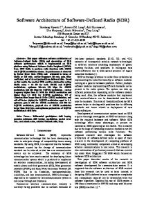
describe their GUI interface. The presence of C++ aids the user to obtain high performance above more compute intensive paths, taking advantage of processor extensions like vector operations. GNU Radio make an extensive usage of a library called Volk, which implements vector extensions. For each method exposed, are available different implementation. Benchmarks are executed in order to understand which instruction is the best choice in different scenario, taking into account size, memory alignment, etc.. The presence of Python allows the user to write code at higher level, interconnecting various basic components. C++ blocks are visible from Python thanks to a wrapping system based on SWIG GNU Radio natively support a large set of protocols, including AM, FM, 802.11, GSM, RFID, etc. New blocks can be simply download or written by the user. Is also possible to create a processing block as a composition of already existing blocks, constituting a sort of hierarchy. In order to receive the FM commercial radio is sufficient to sketch the following flow graph.

Figure 1.1: Flow graph of a FM radio receiver

GNU Radio can be used with external RF hardware, which can be replaced by other purely software blocks in order to executed a completely simulated environment. The task of a SDR receiver antenna is to receive a radio signal, sampling it and eventually translating the frequency, sending the complex samples to the computer in order to be elaborated. The SDR transmitter makes the opposite task. From the Fourier Transform properties, we know that in order to translate

4

CHAPTER 1. SOFTWARE DEFINED RADIO

the frequency of f0 , is sufficient to multiply the signal by e2iπtf0 = cos(2iπtf0 ) + i sin(2iπtf0 )

(1.1)

It means that the incoming signal is multiplied by a cosine and sine, both results are sampled via an A/D converter and outgoing flows are interpreted as the real and imaginary part of the signal, respectively.

Figure 1.2: Complex sampling of received signal

1.2

Hardware

This section show some hardware compatible with GNU Radio.

1.2.1

USRP

Universal Software Radio Peripheral is a family of products initially developed by Matt Ettus. The platform is composed by a motherboard which include an FPGAs, different ADCs and DACs for RX and TX channels, clock generation and synchronization, ending with interface for the PC (USB or Gigabit Ethernet). Is possible to perform analog conditioning (like up/down conversion and anti-aliasing filtering) of the signal through auxiliary cards called daughter-board. Thanks to this modularity, the USRP can operate among a wide range of frequencies, from DC to 6 GHz.

1.2. HARDWARE

5

The board is capable to digitize signals with a rate of 64 MSamples/s with a precision of 12 bit. Is also capable to emit 128 MSamples/s with a precision of 14 bit. The presence of FPGA permits the usage of the board in standalone mode, nevertheless is possible to perform distribute the execution of code between internal FPGA and CPU of a PC connected via USB (or Gigabit Ethernet). This card has good characteristics, but the price is in the order of thousands of euro. In addition, the FPGA has a finite computational power, therefore in some scenario would be great to offload the execution on other devices (like GPU). The interface between USRP and final PC is called UHD.

1.2.2

UHD

UHD is a short for USRP Hardware Driver. It provides an homogeneous interface for all USRP products, is compatible with major OS (Linux, Windows and Mac) and is supported by several framework. Most important are GNU Radio, MATLAB, Simulink and LabVIEW, in any case are exposed APIs accessible from all products with native support for C++.

1.2.3

RTL-SDR

Few years ago Eric Fry discovered that some cheap DVB-T dongles offers direct access to samples captured by antenna, at the desired frequency and without additional elaboration. With 20 eis possible to buy a dongle (based on Realtek RTL2832U) able to receive almost every frequency between 22 and 2200 MHz , with little variation according to the model and some discontinuity near frequency multiple of internal local oscillator. The sampling can be performed at a maximum rate of 2.56 MSamples/s with complex samples of 8 bit. Are available higher value of sample rate, but they can loss samples. Initially were implemented programs able to basic tasks, like receive FM commercial radio on Linux or save samples into files, for a successive elaboration with Octave or MATLAB. Subsequently was implemented a GNU Radio block able to handle these device and make available samples for successive elaboration, directly inside the framework. With a radio receiver with limited characteristic is still possible to perform interesting jobs, like receive audio signals, capture low rate data transmis-

6

CHAPTER 1. SOFTWARE DEFINED RADIO

sions, sniff radio remote controllers and telemetry, capture NOAA weather satellite images and detect pulsars (another limitation is given by the antenna).

Chapter 2 CUDA CUDA, which is a short of Compute Unified Device Architecture, is a parallel computing architecture developed by NVIDIA for massively parallel highperformance computing, exploiting the power of GPGPU.

2.1

GPGPU

General Purpose GPU is an evolution of graphics processing unit (GPU), originally developed for computer graphics, able to perform elaborate a wider set of applications, usually handled by CPU. The CPU was initially developed with an architecture for sequential operations. It uses a sophisticated control logic in order to manage the execution of different instructions out-of-order with multiple function units, still maintaining the appearance of a sequential execution. It also adopts large caches in order to minimize the bottleneck caused by the RAM. Conversely, the main goal of GPU was to execute large amount of floatingpoint operations in order to perform graphic applications. It is composed by several processing units (up to hundreds at least), each one with a simpler implementation and lower frequency respect to CPU. In the first period, the behaviour of these units was hardwired for graphical operations, allowing the programmer to use only languages as OpenGL and DirectX. In last years the interest about general computation performed by GPU grown significantly, leading to a new architecture: General Processing GPU. These graphic cards are able to handle hundreds of threads together, with 7

8

CHAPTER 2. CUDA

a speedup of one of two order of magnitude. In addition they have a good ratio flops/energy respect to traditional CPUs. The main drawback is that is not always easy to port a serial application on GPGPU. In several case performances are worse than CPU. Most common language for GPGPU are CUDA and OpenCL.

Figure 2.1: CPU and GPGPU architecture

OpenCL is an open standard for heterogeneous computing maintained by consortium Khronos Group. It runs on graphic cards of several vendors, over CPUs, DSPs and other processors. CUDA is a parallel computing platform and programming model invented and developed by NVIDIA. It runs only on NVIDIA’s cards, limiting the portability. For my project I’ve chosen CUDA because I’m more skilled with this language. In addition, portability of OpenCL doesn’t imply good performance across different vendors.

2.2

Consideration about CUDA architecture

Now we need to examine some characteristic related to CUDA memory hierarchy, level of parallelism and hierarchy of execution, ending with mechanism for synchronizations. According to NVIDIA convention, we use the term host when refer to CPU and relative RAM, while we use device for GPGPU and VRAM.

2.2. CONSIDERATION ABOUT CUDA ARCHITECTURE

2.2.1

9

Execution

The programmer writes functions, called kernel, which are executed N times in parallel when launched, by N different CUDA threads. Is defined an hierarchy among computation elements. The lower level is the thread, which execute an instance of the kernel, is characterized by a unique ID within its thread block and own a small set of private registers. Thread is executed by a Streaming Processor (SP), which contain an ALU, a Floating Point Unit and other functional units. The middle level is the block, which is a set of concurrently executing threads that can cooperate among themselves through synchronizations and shared memory. A thread block is characterized by a block ID within its grid. Threads of the same block are executed on the same Streaming Multiprocessor (SM) for the entire execution. SM is a SIMT (Single Instruction Multiple Threads) processor which manages and executes threads in groups of 32 parallel threads, called warp. Every SM is composed by multiple Streaming Processor and Special Function Units (SFU, deputed for functions like trigonometric). Actually each block can contain a maximum of 1024 threads. The higher level is the grid, which is the set of all blocks created by a kernel launch, eventually executed on different SM. They are executed independently, the communication can happen only through global memory, that we’ll see later. Is important to remark that threads of same warp execute same instruction ”simultaneously”. If one or more threads executes conditional code that differ in code path from other threads in the warp, these different execution paths are effectively serialized, as the threads need to wait for each other. This phenomenon is referred as thread divergence and dramatically worsen performances. A GPGPU can manage more threads (and blocks) than available SPs (and SMs). Only some warps (and block) are active and a fast context switching happen every time there is a stall due to operand not ready. A common metric of utilization is occupancy, which is the ratio of the number of active warps per multiprocessor to the maximum number of warps that can be active on the multiprocessor at once. There is a finite memory inside the multiprocessor, so higher occupancy implies less registers for each thread. When the kernel is memory bounded (access to global off-chip memory) a good approach is to have high occupancy, because in this way the latency can be hidden switching to other warps, exploiting the Thread Level

10

CHAPTER 2. CUDA

Parallelism (TLP). The drawback of this method is that it aggravate register pressure. Another way to increase parallelism is given by Instruction Level Parallelism [3]. This strategy can be applied with a low occupancy, which implies more registers available for each thread. Programmer must write kernel code which is not stalled waiting data from (immediately) previous instructions like arithmetic and memory transfer (e.g. loop unrolling). Another advantage of this technique is that shared communications can be reduced, because now each thread elaborate more items. This is good, because memory access to local memory is (usually) faster than shared memory, improving the final speedup.

2.2.2

Memory

During execution, CUDA threads can access data from multiple memory spaces. Threads own a private local memory, which is stored in register (access in few cycles, but limited space) or in global memory (off-chip, high latency). Thread blocks have a shared memory visible to all threads of the same block. This is the main method used for communication inside block and accesses are 3-6 times slower than local register (it depends on architecture). Another way would be the usage of shuffle instructions, unfortunately they are not supported by my graphic card. The shared memory is divided into equally-sized memory modules, called banks, which can be accessed simultaneously. If a memory request (usually launched by a warp) contains two or more addresses of the same bank, a bank conflict occurs. In this case the request is split, slowing down performances. Threads can also perform read/write operations on global memory, which is hosted outside the chip (this won’t be true with next architecture Pascal) and survive across different kernel calls. This storage has a capacity in order of gigabytes, but the latency is hundred of times higher than on-chip registers, also bandwidth is slower than storages previously analyzed. Every access is performed with memory transactions with a width of 32-, 64- or 128-bytes. For this reason is important that all threads of the same warp access to aligned and adjacent memory location, otherwise memory access is serialized into multiple memory transactions. The access is called coalesced when this rule apply. Another bottleneck is given by partition camping[4]: as shared memory,

2.2. CONSIDERATION ABOUT CUDA ARCHITECTURE

11

also global memory is divided into memory banks (with a size bigger than shared). When different warps access to the same bank, accesses are serialized slowing down the execution. This limitation was almost solved for Fermi and newer architectures. Two other kind of memory are texture and constant. The former is useful in graphics application because allow the programmer to use floating point indices over matrices, performing an efficient interpolation across adjacent cells. The latter allow an efficient access to constant memory, but loads must be relatively small and must be accessed uniformly for good performance (All threads of a warp should access the same location, otherwise a serialization will be performed). Both kind of memory are hosted on global memory, with on-chip caches for last used values. I’ve decided to don’t use constant memory because its size is very small and it would be shared by different GNU Radio blocks. Inside the chip there is a L2 cache for the global memory, which is almost transparent to programmer (is possible to use PTX instructions in order to interact with it, as also with L1). It is visible by all SMs into the chip and it uses a LRU policy. This memory is also used to perform Each SM has an own L1 cache, which is stored on the same memory portion of shared memory (on newer architectures is possible to choose how split this space). According to the architecture, this cache is used for all accesses to global memory or only for register spilling. Last architectures provide an efficient mechanism for constant memory, called read-only data cache. It can be enabled by compiler over standard pointers pointers when certain conditions are met, like the usage of modifiers const and restrict . It uses a separate cache with a separate memory pipe (to global memory) and with relaxed memory coalescing rules. The usage of this feature can improve the performance of bandwidth-limited kernels, because data cache can be much larger and can be accessed in a non-uniform pattern respect to standard constant memory. CUDA kernels can access directly to host memory regions when the allocated RAM is pinned (guarantee that the memory page is not flushed onto hard disk) and mapped into device address space. This feature is called Unified Virtual Address space (UVA). From CUDA 6 this feature was extended with Unified Memory, which eliminates the need of explicit data movement between host and device memory. Memory regions are automatically migrated where they needed (also across different devices in multi GPU configurations), facilitating the pro-

12

CHAPTER 2. CUDA

gramming and maintainability. Actually a clever ”manual” management is much more efficient than this mechanism, so I didn’t use this feature in my project. Operations Main operation is the memory copy between host memory (RAM) and global memory (cudaMemcpy and cudaMemcpyAsync). Surely the bandwidth is upper bounded by PCIe bus. Another limit is given by the kind of allocation in host memory. If the memory region is pinned (page-locked), the allocation cannot be swap onto secondary storage and the the copy is performed directly by the DMA. Otherwise the host need to perform an additional copy between the host memory and an internal host-pinned memory, halving the bandwidth. Recent architectures contain one or more copy engine, which allow the contemporary data transfer and execution of independent kernel. Memory copy between host pinned memory and global memory can also be performed writing an adequate kernel. Choosing a clever occupancy and ILP is possible to reach same performance of the CUDA memory copy function (from my experiments), where the bandwidth is limited by PCIe bus. CUDA provides a function for memory initialization, called cudaMemset, which allows the user to fill/initialize an array. The curios fact is that this operation doesn’t fulfill the bandwidth. Is more efficient to write a small kernel in order to perform the initialization. The CUDA API is used where the initialization is performed only once, at start-up.

2.2.3

Concurrency and synchronization

Scheduling of kernels An important concept in CUDA is stream. It is a sequence of operations that are executed sequentially, while commands of different streams may be executed out of order and concurrently. Kernel calls and memory copy are always associated to a stream, implicitly or explicitly. Example of explicit usage of stream are CUDA functions that contain async in the name, like cudaMemcpyAsync. A particular case is the default stream, which issues next operations when all previous commands from any streams (of current threads or all threads)

2.2. CONSIDERATION ABOUT CUDA ARCHITECTURE

13

are terminated. This is used as implicit stream. The host code can pause until previous command in the stream are executed, providing an useful mechanism of synchronization. An interesting object is event, which monitors the device’s progress as well as perform accurate timining. Events are inserted into a specific stream (may be the default stream) and are recorded when all previous command in the queue are executed. Host code can query their status in order to know the progress, is also possible to suspend host execution until a given event is recorded. Streams can be paused until a certain event is reached, providing an useful mechanism to wait the availability of all inputs before a kernel execution. Combining streams and events, is possible to express a direct acyclic graph of dependencies. If a stream A should wait that stream B reach a given point, is sufficient to create an event associate at this spot and pause the execution of A until the event is recorded. The graph is acyclic because is not possible to pause a stream waiting for an event not still created when CUDA schedule it (from host side). In this case the execution continue ignoring the conditional pausing. Warp execution Threads of same warp execute simultaneously and CUDA provides some mechanism for synchronization across warps. There is a basic barrier synchronization for warps of same block through the function syncthreads(), that pause thread execution until all warps (of block) reach the barrier. This is a rigid mechanism, because in lot of case is undesirable to wait every threads. This happens each time the function is called inside a branch imposing a more complex code to the programmer. The barrier also strongly limits application where each warp takes a different execution path (warp specialization) The ”assembler” of CUDA offers a more flexible mechanism inside the block , called named barriers . Are available 16 barriers and the syncthreads() is built on it, using two of them. There are two methods, one signal the arrival of a warp to a given barrier (without stop), while the other stop the warp until a certain number of warps has signaled its arrival to the barrier. Using two barriers, is possible to implement a producer-consume paradigm over different warps. This feature is exploited by CudaDMA [5] library, which provides an

14

CHAPTER 2. CUDA

higher level approach (respect to manual handling of PTX code) for execute asynchronous memory operation. Warps are split in compute and memory groups, one performs elaboration and ask to load new data, while the other perform memory global operations. This can be very efficient when the memory pattern is not sequential. Is not available a function for synchronization across threads of different kernel. Researcher suggest some approach like memory spinning, but is not guarantee that they work in every conditions. The scheduling is not predictable or the same for all architecture, so a code that perfectly work in one graphics card, cause deadlock on another.

Chapter 3 SDR with CUDA 3.1

State of art and objectives

The usage of software defined radio could require an huge computational power during elaboration, which can be speed up thanks to the usage of GPGPU. Actually there are some implementations of radio processing blocks which take advantage of GPGPU capabilities. Gr-theano[6] is a module of GNU Radio which uses a Python library, called theano[7][8], strictly integrated with Numpy. Currently this module is able to perform FFT, FIR filtering and can be used to model the fading. Gr-fosphor is a block which shows a waterfall diagram of the input, using OpenCL in order to compute the spectral components and OpenGL for the visualization. Some years ago was also available an experimental library called gr-gpu. The author was not satisfied about its performances and removed it from repositories. I was not able to find the source code. Another useful example is an implementation of LTE receiver [9] over GPGPU. Their research was more focused on turbo decoder, their implementation takes globally few milliseconds for each data frame sent/received, being able to work in real-time. The problem is that previous implementation, although they provide good performance, are very specific for a specific target and are not able to provide a flexible framework, losing the wide approach given by SDR. The goal of this thesis is to extend GNU Radio in order to allow users to 15

16

CHAPTER 3. SDR WITH CUDA

build flow graph composed by CUDA blocks, finding and minimizing bottlenecks. The porting will cover all the main blocks,so mathematical operation between flows, low-pass/high-pass/band-pass filters, IIR filters, FFTs and FFT filters, ending with OFDM. The final user should be able to use these blocks without an additional knowledge. The unique suggestion is to avoid the insertion of CPU GNU Radio blocks between GPU blocks. For compatibility reason I’ve decided to don’t make a customized version of GNU Radio, instead I’ve created a module which contain all blocks and management. This module can be imported in every installation which support CUDA, immediately after can be used joined with other blocks. For sake of simplicity this framework won’t be compatible with CUDA device characterized by a compute capability less than 2.0. Older architectures are very limited, in addition its support is ended with CUDA 7.0. In this thesis I start showing the common part used by all my blocks (management of memory, execution, etc.) followed by choices in the design of single blocks.

3.2 3.2.1

Architectural choices Memory

The management of memory is always a problem: each transfer between host and device is expensive in terms of bandwidth and latency. For instance the computation of FFT over the CUDA device can be very profitable, but part of the gain would be lost if the FFT size is small, the input and output must be transferred from/to host memory and a low latency is required. Is mandatory to minimize transfers between device and host memory. Ideally there is only one transfer host-to-device at the beginning of the flow graph (e.g. incoming data from antenna) and a device-to-host copy at the end. Now we examine requirement of GNU Radio blocks in terms of communication buffer between adjacent blocks. In a data-link between to attached blocks, we call top the source of data and bottom the sink of data flow. We know that some block has a simple relation 1:1 between incoming and outcoming data, while other has N:1 (decimation) or 1:N (interpolation), where N is previously know. Where are rarely case in which N is not previously

3.2. ARCHITECTURAL CHOICES

17

know (e.g. frame detector) because it depends on incoming data and the size must be returned from device, but we can manage this case separately. In addition some blocks has special needs, like know previous inputs(history) for blocks like FIR filter, in other case is necessary to know previous outputs (e.g. IIR filter). It is also recommendable to don’t invoke a kernel over a small task, otherwise overhead due to invocation would be greater than computational time. A first approach would be the usage of a circular buffer allocated in device memory at start-up. It satisfies some requirement, but the code would become complex when we try to use the same buffer as input for one block, and both input/output for another blocks. In addition, it would impossible to make a clever usage of CUDA events in order to manage a producer-consumer pattern on the device. A good trade off would be the usage of a circular buffer of pages, where each pages is an area in device memory with a dimension of some Kilobytes or Megabytes. The number of pages and the dimension of each would be a tradeoff between latency and execution time. Each page is associated to two events: one is registered when the write operation (by the producer) on the relative page is finished, while the other is registered when the read (from consumer) is terminated. At the beginning (in the constructor), each blocks declare its preference of incoming and outcoming links, like minimum and maximum number of items per page, which multiple should be the number of items in the page, maintain the previous page as history. This strategy aims to improve memory usage. Each block must perform, for each invocation, a method called polling which internally manages the initially handshake and each time performs different checks. All information about current written/read page and its length are contained in host memory, because the CPU knows and uses these information (e.g. when is necessary to split a kernel call in two separate execution, due to end of page of output). Lot of blocks have the dimension of output predictable from the input size, so it can calculated by host, avoiding expensive memory transfers. There are two GNU Radio blocks for the memory transfer between RAM and memory device. They perform a series of cudaMemcpyAsync between GNU Radio buffer and CUDA buffer. Unfortunately the host buffer is not pinned, so we cannot avoid the double-copy, halving performances. In any case is possible to use cudaHostRegister in order to pin these buffers, but

18

CHAPTER 3. SDR WITH CUDA

their structure is not guarantee to remain stable with next version of GNU Radio, so I’ve decided to don’t enable it. Usually the transfer rate is not the biggest challenge in SDR if transfers are used sparingly (e.g. transfer the flow coming from an antenna with a bandwidth of 20 MHz needs about 160 MB/s, while each graphics cards support a speed at least one order of magnitude greater). The GNU Radio buffer is not pinned, but is possible to take advantage from asynchrony: time spent by memory transfer can be hidden executing it in parallel with other computations.

Figure 3.1: Circular buffer of samples pages and tags

3.2.2

Execution and synchronization

Each block launches one or more kernels for each incoming page. Launches can be synchronous or asynchronous. In the case of synchronous, at the beginning the polling method transparently waits the termination of kernels launched in previous blocks. This seems not strictly necessary, due to the fact that null stream wait the termination of kernel previously launched in any streams. But we need to manage also the read event, otherwise the previous block can potentially overwrite a page not completely read, due to the asynchronous termination of synchronous kernel call. Successive blocks wait the termination of kernels executed in the synchronous block (otherwise it would read page not completely written). In case of asynchronous, each kernel launch is associated to a different CUDA stream. Before the launch, the stream waits the events of write com-

3.2. ARCHITECTURAL CHOICES

19

pleted about current input page and read terminated about current output page. subsequently the kernel launch, are inserted in the queue of current stream the creation of two events: output page written and input page consumed. In this way is possible to execute at same time different kernels, expressing input/output data dependency directly over the device. With this approach is possible to reduce the gap between kernel execution of adjacent blocks to 2-3 microseconds, instead of hundred or thousands of microseconds required by synchronous approach (due to CUDA and Python overhead, which is now hidden). Kernels of adjacent blocks are subjects to dependency, so is a good approach to have, for each invocation of our block, multiple page (it means multiple kernels launches) which need to be elaborated. In this way is possible to keep busy all Streaming Multiprocessors (SM). One of the weak point of CUDA architecture is what kernel calls are serialized on the scheduler, so is possible that an SM is not working,also if there is a ready kernel, because before this kernel was launched another which is still waiting an event. This limitation is partially overcame in recent NVIDIA cards with a technology called Hyper-Q, which provides multiple hardware queue. Now the main task of CPU is to schedule tasks over CUDA card, filling queues. It is important to limit number of kernel shedulations performed by CPU, otherwise the processor will fill completely the CUDA task queue. This is solved putting some sort of synchronization on all blocks that produce more output pages that consumed input pages. Every time that one of these blocks has scheduled kernels for all pages (of circular buffer), it cannot schedule new tasks until previous elaborations are performed.

20

CHAPTER 3. SDR WITH CUDA

Chapter 4 Implementation of common parts 4.1

Tagged streams

GNU Radio was originally developed as a streaming system, where data flow between consecutive GNU Radio blocks is treated as a stream of numbers. They represent samples provided by antenna, inputs for the audio sink, etc. This basic model doesn’t provide features like control and meta data over the data flow. In different scenario would be useful to associate meta data to these values, like time stamp of receipt, frequency, beginning of a new packet (in OFDM transmission). In order to satisfy these requirement, GNU Radio provides a feature called stream tags. This is an additional data stream that works synchronously with the main data stream. Tags are generated by specific blocks, are associated to specific samples and can follow the same flow of the main data flow. Each blocks can propagate, ignore, modify or add tags. Each tag is characterized by a key-value pair, both fields are PMTs (Polymorphic Types). PMT is usually used to carry numbers and strings, but it also support dictionaries, tuples, vectors of PMTs and other types. In practice, only strings and numbers (integer, float, complex) are used as PMT, so I’ve implemented these cases. In addition, the management of textual keys in parallel can be a bottleneck. For this reason, textual keys which are treated by blocks on GPGPU are transparently converted to numerical constant during the memory transfer 21

22

CHAPTER 4. IMPLEMENTATION OF COMMON PARTS

between host and device (and vice versa). Other textual keys can be managed as bunch of bytes, because are meaningless for blocks executed over GPGPU. Blocks can ignore tags, forward them directly (e.g start of frame) or modify them. Lot of blocks don’t use tags, but eventually propagate them. Given a page of samples to a GNU Radio blocks, is not predictable the number the number of tags that will be produced by the block itself: it is known from the kernel function only during the execution. In addition, we’d like to maintain the asynchronous kernel execution for performance reason. In a typical case the block at the beginning of flow graph produces tags, which are propagated and consumed only at the end of the chain. A situation like this is not rare. For this reason is not good to use an approach similar to the main data stream between consecutive blocks (a circular buffer of pages), because in the worst scenario we would have tons of avoidable memory copies. A better approach would be to ”allocate” a memory region each time that is necessary to associate tags to some samples. For sake of simplicity, all tags of samples contained in the same page (referring to buffer of main data stream) are maintained in the same memory region, which we call tag page. So each page of circular buffer is eventually associated to a different tag page. The forward is performed simply by propagating the pointer to the next GNU Radio block. What happen then a block needs to modify/add/delete some tags? Before to think how to implement this situation, is better to consider another scenario.

4.1.1

Usage of reference counters

Is possible that a block propagates incoming tags to multiple output, then is preferable to avoid additional memory copies (due to bifurcations). It seems obvious the usage of reference counter for each tag page, which are incremented each time that a tag page is propagated to multiple outputs. When a tag page is modified, a new tag page is created and is propagated to next blocks, while the reference counter of source tag page is decremented. In this way, there are no problems if a block in a branch modify the tag page shared with another branch. The unique case in which is not required to create a new page is when the reference counter is equal to 1, but usually performed operations are add and delete tags. It means that in lot of case is required a different size for the tag page, so an allocation would be necessary.

4.1. TAGGED STREAMS

23

Each time that a tag page is not propagated by a block, the relative counter is decremented. When it reaches zero, the tag page can be deallocated. Because kernels are executed asynchronously, is necessary to wait the kernel termination before to decrement the counter. This requirement can be accomplished in different way. • CudaStreamAddCallback called after the invocation of CUDA kernel, performing the decrement of counter • Create an event when the kernel terminate. Probe sometimes events happened (tag page is consumed) and decrement relative counters. The first approach has some limitations, like the callback method cannot contain CUDA calls (like cudaFree) otherwise in some situation a deadlock can happen. The execution of the callback method is expensive (about 15 microseconds on my platform) and prevents the occupation of all streaming multiprocessor (because there is a sort of synchronization between device code and host code). The latter consist of create a CUDA event after the termination of CUDA kernel with cudaEventCreateWithFlags (in order to don’t save timing information, which slowdown the execution) and cudaEventRecord. Sometimes cudaEventQuery is called in order to test which events are happened, in order to know which tag page can be deallocated (or reference counter decremented). This approach allow to call CUDA API during deallocation, like cudaFree, because is not a callback method like the previous. Are used three Nvidia call, cudaEventCreateWithFlags, cudaEventRecord and cudaEventQuery, which take between 0.5 and 1 microseconds each, with an overall overhead between 2 and 3 microseconds. This implementation would be faster than CudaStreamAddCallback, but it can be improved. Is not mandatory that the reference counter is decremented immediately after the execution of kernel which consume the page. In addition, we know that all CUDA calls executed on the same stream are performed sequentially. In order to decrease perceived overhead due to CUDA API calls, we can use a time-space tradeoff: record (and create) an event every N CUDA kernel termination (over the same stream). In this way, the overhead is reduced by a factor N, increasing the number of tag page which are not anymore referenced, but are still in memory.

24

CHAPTER 4. IMPLEMENTATION OF COMMON PARTS

4.1.2

Considerations about allocation

In some case the size of tag page is predictable by the host before the kernel launch, e.g. during the copy of samples between host memory and device memory. In other scenarios the number of tags is know only during the execution of CUDA kernel, for instance when the kernel detect the beginning of packets. The problem is which allocator use in order to create memory regions over device memory. Adopt only an host malloc is not easily implementable with asynchronous call, because after the kernel execution (which produce tags) would be necessary to allocate a memory region and copy tags inside. Is not possible to call asynchronously a cudaMalloc (inside a CudaStreamAddCallback), so a customized allocator would be necessary. The usage of callback is also a nightmare for performance. Is not a good idea to adopt only a device malloc, because in scenario like move data flow (of GNU Radio flow graph) from CPU to GPU sizes are known by CPU (because its copying tags from RAM). Is better to allow the user to use both. Each tag page is referenced by an ”handle”. It is composed by a reference counter, a flag which indicate the used allocator and a pointer to device memory (allocated by host). This pointer refers to a small memory portion, what we call kernel pointer, containing only the address of the tag page (on device memory). Kernel pointer can be written by host and device without problems about performance. kernel calls need only to access to this pointer, without interact with host memory. At the same time, the host code only need to propagate handles between GNU Radio blocks, also when the tag page is NOT still allocated.

4.1.3

Allocation

Because for each page could be necessary to allocate space for tags, invocation of allocation and deallocation in memory can happen often, that induce a significant bottleneck. There are different kind of allocation on device memory: • Fixed size by host • Flexible size by host

4.2. MEMORY ALLOCATOR

25

• Flexible size by device The former usually doesn’t involve big chunks of memory and is used especially for allocate kernel pointer. An approach would be to allocate at the beginning a big chunk of memory, splitting it and putting pointers into a free list. Malloc is performed by taking (and removing) a pointer from this list, while the free is performed by inserting the pointer inside the list. Memory allocation by host with flexible size can be easily performed by cudaMalloc, while the free can be executed via cudaFree in some lazy way (callback cannot be used). The allocation of one million of region with the size of one pointer takes about 10 seconds, it means 10 microseconds for each allocation. The cudaFree takes other 6 microseconds, plus a big drawback: this function waits the termination of previous calls executed on device, impeding the asynchronous paradigm. In the next section we explore a customized allocator. For the last case (allocation from device), are available the CUDA malloc() and free() methods. Their performance are acceptable when they are used sporadically and not concurrently from different threads. Are available specific allocators like Halloc[10] with high performances, but they’re designed for small allocations. In my project, allocations performed by device are minimized.

4.2

Memory allocator

In our implementation there are lot of device memory allocation/deallocation performed by the host. As seen previously, these API calls are expensive in terms of performance. For this reason, it would be great to use a customized allocator which manages device memory and makes few interactions with CUDA allocator. There are different types of allocator: in my implementation I’ve chosen a memory pool which offer only memory regions with size power of two, because is simple and faster compared to other approaches. The maximum internal fragmentation will be not bigger than the space required by the user. In addition, are available additional sizes which accommodate objects largely used, like kernel pointers. Another requirement is that calls to allocator are thread safe, because each GNU Radio block can work in a different threads. Usually memory

26

CHAPTER 4. IMPLEMENTATION OF COMMON PARTS

allocated by a block will be deallocated by another block, then would be preferable to share freed allocation among all threads.

4.2.1

Structure

Each GNU Radio block instantiate a set of Allocator object (one for each size). These objects contain a set of free allocations. All malloc/free operations take/insert pointers in this set. When the cardinality of the array is lower/bigger than certain thresholds, a subset of pointers is taken/moved from another object, called GlobalAllocator. It is a templated singleton, where the parameter is the size of memory region. It means that there is a unique global object for each size, uniqueness that is guarantee by a c++11 construct. It shares a set of free region with local allocator, allocating new space when necessary.

4.2.2

Optimizations

There are different C++ data structures which can host the set of pointers. The more suitable are vector, list and deque. I’ve tried all three approach, but the first is always faster, also with GlobalAllocator which need to copy some hundred of pointers each time. I’ve also tried a mixed approach: local allocators work with vector of free portions, while global allocator keep a list of vectors. In this way, for each interaction with a local allocator, an item of the list (vector of pointers) is inserted/removed. This approach tend to be slower than the simple vector. Is mandatory to guarantee multi threading, while at the same time is desirable to minimize its cost. It would be great to minimize temp spent inside locked sections. Methods malloc and free of global allocator(which work on vectors of pointers) are protected by a lock guard, according to RAII paradigm (Resource Acquisition Is Initialization). This mechanism is provided by Boost and by c++11 standard libraries. Boost is faster on my machine, in any case the price paid for critical section is distributed among multiple allocations. Each local allocator keeps two vectors of free allocations, operations are performed above one, called active. When the active vector contains more pointers than a given constant, vectors are swapped. When both sets are full, one of them is passed to global allocator, while the other become the active set. This transfer of items (pointers) and the opposite operation (get

4.2. MEMORY ALLOCATOR

27

allocations from global allocator) are performed using the move construct of c++11, which move the ownership of an object. In this way is not performed a useless copy of objects (during the passage of arguments) which are demolished immediately after. The compiler can also get more advantage respect to the usage of references.

4.2.3

Performances

Sizes of memory pools used by local and global allocators can be changed easily. In my implementation, I’ve chosen for the global pool a minimum size of 4096 items, while local pools are between 512 and 1024. I’ve tried to executed for 100 000 times a set of 10 000 allocations followed by their deallocations (but performed from a different local allocator). In this way local allocators need to interact often with global allocator. The whole execution for one billion of allocation/deallocation takes between 5.6 and 5.7. It means that in average a pair allocation/deallocation takes less than 6 nanoseconds, much better than microseconds required by CUDA allocator.

28

CHAPTER 4. IMPLEMENTATION OF COMMON PARTS

Chapter 5 Basic blocks Is important to give the opportunity to perform basic tasks as mathematical operation over signals. GNU Radio provides blocks for each operation, all implemented using the most appropriate CPU vector extension. I’ve written an implementation for addition and multiplication(signal-to signal and signal-to-constant), division and amplitude of complex number. We can expect tasks memory bounded, with a short kernel duration.

5.1

Addition and multiplication with constant

Implementation and behaviour of these blocks is expected to be similar. Where don’t specify, I speak about summation between complex numbers and each input page has a size of 4 millions of samples (MSamples). The kernel of the naive implementation takes about 6.8 ms for each execution, with the best combination blockDim and gridDim, with an occupancy of 100%. In this case, accesses performed by a single thread are strided with size of grid. Adding a pragma unroll above the loop decrease performances. For complex numbers, an idea can be to use even threads for real parts and odd threads for imaginary parts, with manual overlapping in order to execute the same number of operations (for iteration) of previous implementation. According to profiling, kernel execution become slower. Computing two items for each iteration with a manual unrolling of two operation (with size blockDim inside the loop), is possible to terminate the execution in 3.2 ms (occupancy 85%), doubling performance also thanks to better locality. According to the profiler, global bandwidth is near the limit 29

30

CHAPTER 5. BASIC BLOCKS

(>24GB/s), but there is an unbalance of 30% between global loads and stores. It seems natural to improve locality by splitting the input page in gridDim parts. Global bandwidth is slightly smaller (25GB/s) than the device limit, with a good balance between reads and writes, but surprisingly the time execution doubles. The best option is a manual unrolling of four operations inside the loops, with an additional pragma unroll over the loop and without the tiling of input page across blocks. This kernel is executed in 2.64ms, with an occupancy of 66%. Global bandwidth is 19GB/s, while L2 bandwidth is near the limit. A manual unrolling of 8 items doesn’t improve results. Is important to remember that in the flow graph there are some blocks which stops when where are too much scheduled tasks. This mechanism requires a sort of host-device synchronization which is costly and allow each GNU Radio blocks to schedule over a limited number of streams. This problem is hidden when there are different GNU Radio blocks (each using CUDA) or when each kernel execution takes more than 5 ms (this number is very flexible). In this case the duration of each kernel is the half, so the GPU elapses half time in idle.

GPU CPU GPU

40 Time(s)

Seconds

20 15

20

10 5

0 1

2

3

10 10 10 Thousands of samples per input page

8 16 Length input (GSamples), each page contain 4MSamples

5.1. ADDITION AND MULTIPLICATION WITH CONSTANT Length input page Length input 16k 8G 64k 8G 256k 8G 2M 8G 4M 8G CPU 8G 4M 16G CPU 16G

31

Time 20.3s 5.6s 4.14s 4.13s 4.06s 24.7s 6.91s 49.4s

The bar chart considers input pages of 4 MSamples and is noticeable a speed up of 6-7 times for complex addition (respect to CPU). There is an exception for input pages with small size (16 thousands of samples). In this case, most time is spent in idle. In a real scenario this rarely happens, because there are also other blocks filling CUDA queues. The naive implementation of multiplication requires 11 register for thread and has an occupancy of 100%. The elaboration of 8 billion of samples takes 7.1 seconds (7.5ms each kernel execution). I’ve performed experiment similar to addition and the best implementation is the same again, manual unrolling with stride access of blockDim inside the iteration and blockDim*gridDim between iterations. Each threads occupies 27 registers and the occupancy decrease to 66%. The execution time over the same previous elaboration takes 4.85s (with manual unrolling of 4 items) with a speedup of 46%. Using a manual unrolling of 8 samples improve slightly the execution, going down to 4.18s (+16%), while the execution of single kernel is accelerated by 31%. Below are shown results for complex multiplication by constant.

32

CHAPTER 5. BASIC BLOCKS GPU CPU

Time(s)

150 100 50 0 4

Length input (GSamples)

Length input page 4M CPU 16k 64k 256k 2M 4M CPU 8M

Length input 4G 4G 8G 8G 8G 8G 8G 8G 16G

8

Time 2.75s 71.3s 28.2s 7.51s 4.21s 4.20s 4.18s 143s 7.23s

In this scenario the GPU strongly dominates, reaching a speedup of 34x. Is mandatory to keep in mind that complex multiplications can exploit better Instruction Level Parallelism. With 16 billions of floats, CPU takes 69.8s and GPU 5.86s, with a gain of 12x. Similar situation happens with integers, with a speedup of 11 times.

5.2

Magnitude of signal

A common task in DSP is to get the magnitude of a complex signal. GNU Radio provides two blocks, one calculate the normal magnitude, while the other emits squared magnitude.

33

5.2. MAGNITUDE OF SIGNAL

I’ve decide to implement an unique block, that takes in input a generic exponent (it must be a natural number). Due to limited resources assigned to each thread, I’ve decided to write different specialized kernels, chosen according to exponent. In case of unitary exponent, an implementation would be to calculate the square root of the sum between the power two of real and imaginary parts. Luckily, CUDA provide an intrinsic function called hypot, designed for calculate the hypotenuse of a triangle given its cathetus. The same kernel, already optimized with unrolling is 70% faster with this function instead of explicit computation. With exponent two, the computation is trivial: each output is given by the sum of real and imaginary part, both squared. This implementation require less registers than the previous. Also the computation is easier. For bigger exponents, are available two kernels, one for even exponents, while the other for odds. For each item, they calculate the magnitude (squared for even exponents). Starting from this number is performed the operation N Exp with an exponentiation by squaring, finding the result in O(log2 Exp) steps. This technique calculates only powers of N with exponent power if two. From the binary representation of exp, is easy to understand which powers of N needs to be multiplied together, leading to the final results. This fast exponentiation is vectorized, in order to calculate more powers together. In the next table is show the time spent elaborating 32 billion of items, with an input page of 4 MSamples. In brackets is indicate duration time of each kernel invocation. Exp 1 1 2 2 3 4 31 32 511 512

Platform GPU CPU GPU CPU GPU GPU GPU GPU GPU GPU

Time 24.8s (4.99ms) 73.6s 10.3s (1.79ms) 82.5s 25.7s (5.40ms) 17.8s (3.16ms) 29.4 (5.86ms) 18.0s (3.68ms) 33.5s (6.10ms) 18.4s (4ms)

34

CHAPTER 5. BASIC BLOCKS GPU CPU

Time(s)

80 60 40 20 0 1

2

3

4 31 32 Exponent

511 512

Speedup for normal magnitude is only 3x (CPU uses a single vectorized instruction), while squared magnitude get a 8x. Exponent of 512 is useless in practice (e.g. float type cannot contain it), but is useful to show the slow grow of execution time respect to exponent. The difference in duration between odd and even is explainable by the fact that they use a different number of registers and different launch parameters. Kernels with even exponent can reach a better occupancy, hiding better latency caused by global memory transfers.

5.3

Complex conjugate

That is another common operation, which flip the phase of the signal. The best approach is again a manual unrolling, with an internal stride of blockDim, while the next iteration access to a distance of blockDim*gridDim. The kernel perform 4 million of conjugate in less than 2ms. We bandwidth of L2 cache is completely used, but the ratio load store is not unitary. The execution is able to reach a full occupancy, elaborating 32 billion of items in 10.8s, while CPU take 61s. A possible approach is to modify the range of unrolled loop, splitting input page across blocks. This approach is 5 times slower.

5.4. OPERATIONS BETWEEN TWO SIGNALS

5.4

35

Operations between two signals

These blocks have a similar behaviour and are expected to be memory bounded. For each operation is necessary to load two operand from two separate memory regions, followed by the store of one operand in a third region. Because the operation is easy (expect the complex division), we can expect similar behaviour. I start considering the complex summation and the considered input page size is 4M samples. Addition The naive implementation with the best choice of blockDim and gridDim computes 16 billion of complex sums in 18.2s , which remain similar with the insertion of pragma unroll. A simple manual unrolling with 4 operations (striding inside loop of blockDim) takes 10.6s, with a speedup of 71%. Each kernel is executed in 1.16ms, occupies 30 registers and reaches an occupancy of 67%. With 20GB/s of reading and 15 GB/s of writing, the l2 cache is near its limit. We can also notice that the ratio load/store is not 2:1 as expected. On my graphic cards, the best tradeoff is given by a grid with 6 blocks, each one composed by 256 threads. In the complex addition, real and imaginary part are completely independent (this doesn’t apply to multiplication and division). A possible idea is to treat the complex summation as a float summation, with vector size doubled. Now there are even threads that compute real parts, while imaginary part is elaborated by odd thread. In this way each warp makes global transactions of 128 bytes. Applying this idea to previous implementation (manual unrolling), we obtain a kernel with lighter threads, each uses 18 registers. Now is better to use a block size of 512 in order to reach a full occupancy. The kernel execution time falls to 0.91ms (+27% respect to previous implementation) but the gain in terms of overall time is not so sensible, now it takes 9.78s(+8%). This happens because queue of graphic card is filled only with small kernel, so lot of time is wasted in idle. It can be interesting to see if is possible to improve more the implementation. A common approach used for memory bounded problem is to use vectorized types (as float4 ) in order to increase the bandwidth. Unluckily this strategy performs worse, with a slowdown greater than 40%. An interesting way can be the usage of warp specialization, it means

36

CHAPTER 5. BASIC BLOCKS

that different warps have different tasks. Due to the fact that GPUs execute instructions in-order, it would be nice to load subsequently operands before immediately after the read of current operand, while other warps make computations. CudaDMA is a library which offers this opportunity, using named barriers. The programmer defines which threads perform global loads to shared memory and the pattern, exploiting Memory Level Parallelism.Is possible to launch an async read of next operand before the current operation, pausing current thread when the value is truly necessary, with a producerconsumer paradigm. Unfortunately I was not able to gain performances with this approach, using two specialized groups of warps for global reading of input vectors. Probably the compiler can well optimize my code, inserting some prefetch instructions. GPU CPU GPU

60 Time(s)

Seconds

30

20

10 101 102 103 Thousands of samples per input page

Length input page 16k 64k 256k 2M 4M CPU 8M CPU

40 20 0 8 16 Length input (GSamples)

Length input 8G 8G 8G 8G 8G 8G 16G 16G

Time 28.2s 9.26 6.15s 6.12s 6.08s 31.9s 9.78s 62.7s

37

5.4. OPERATIONS BETWEEN TWO SIGNALS

Complex addition has a speedup of 5-6 times, mainly bounded by memory bandwidth.

Multiplication The basic implementation of complex multiplication performs 16 billion of operations in 20.8 seconds. Each thread uses 14 registers and the kernel performs 4 million of multiplications in 8.86 ms. Ratio between global loads and stores is 1.3:1, while the global bandwidth is near the saturation. For multiplication is not possible to split imaginary and real parts across different threads, so this useful optimization is not applicable. Manual unrolling with 4 operations improves the timing, falling down to 17.3s. The duration of a kernel is about 5.6ms(+58%), with 30 registers/thread. Additional unrolling is not useful. CUDA offers the possibility to perform L2 prefetch through the PTX instruction prefetch.global.L2. I’ve inserted this command at the beginning of unrolled loop, now the kernel takes 5.3ms (+5%), with an overall time of 17.1s. In addition, number of L2 loads and stores reach a perfect ratio 2:1, while global read and writes are nearly. Is also important to remark that usually NVCC compiler doesn’t unroll loops containing PTX instruction, but this is compensated by manual unrolling already present.

Length input page 4M CPU 16k 64k 256k 2M 4M CPU 8M CPU

Length input 4G 4G 8G 8G 8G 8G 8G 8G 16G 16G

Time 5.01s 10.85s 29.3s 9s 8.58s 8.53s 8.53s 22.9s 16.9s 44.8s

38

CHAPTER 5. BASIC BLOCKS GPU CPU

Time(s)

40

20

0 4

8 Length input (GSamples)

16

For complex multiplication, speedup is only about 2.6x. With float and integer multiplications, prefetching seems useless so I didn’t use it. At same time, I’ve applied a manual unrolling of 8 operations. 64 billion of float multiplication are performed in 121s by CPU and 22s by the GPU, with a speedup of 5.5x. Similar results with integers, where CPU takes 156s and GPU 24.1s, with a final speedup of 6.5x. Division The elementary kernel takes 12.5 seconds to perform 4 billion of complex division, with 19 ms for each kernel and 17 registers/thread. The manual unrolling (with 4 operations) brings the overall time to 10.9s (+15%), while the execution of a kernel takes 16.7 ms. The complex division is performed in several step. An idea can be to break each division and reschedule its step, reducing execution dependency (a math operation that wait result of previous operation). Applying this technique to unrolled loop, the overall time become 9.1 (+20%), while each kernel takes about 13 ms (+30%). According to profiler, now the kernel is mainly stalled by instruction fetch, while execution and memory dependencies are less significantly. The chart below show a speed up of about 10x.

39

5.5. FFT OF SIGNAL GPU CPU

Time(s)

150 100 50 0 2

4 8 Length input (GSamples)

Length input page Length input 4M 2G CPU 2G 16k 4G 64k 4G 256k 4G 1M 4G 4M 4G CPU 4G 4M 8G CPU 8G 4M 16G

5.5

16

Time 4.19s 38.3s 18.3 10.5s 9.43s 8.87s 8.36s 76.2s 14.5s 153s 27.1s

FFT of signal

GNU Radio provide the opportunity to perform the Fourier Transform and its inverse over a signal, taking advantage of FFTW library. The user can specify a window of items, that will be multiplied with the signal (before or after the FFT, according to direction). In frequency domain, is possible to have the DC component at beginning of spectrum, or translate it in the middle. This kind of shifted representation is often used. A popular and efficient FFT library is cuFFT, provided by CUDA. It is highly optimized for size writable in the form 2a x3b x5c x7d . Its limitation is that is callable by host, while it can be called by device only supporting

40

CHAPTER 5. BASIC BLOCKS

dynamic parallelism (a kernel launch another kernel), that is not the case of my graphic card. Consequently for each elaboration can be necessary to call a maximum of three different kind of kernels. The first and the last eventually perform a multiplication with the window and a shift of spectral component, they’re called once for each input page. The middle kernel is the execution of FFT, called one or more time. Calls to cuFFT can be asynchronous, which fits with the approach of my framework. Another feature of cuFFT is the possibility to plan and batch multiple FFT transform in one single execution. At start-up, my block creates several plans, for different batch sizes and streams. During execution, the number of cuFFT calls is minimizing using each time the biggest plan that fits with the current input. Input size 16G 16G 16G 16G 16G 16G 16G 16G

FFT size 64 64 256 256 1K 1K 4K 4K

Platform GPU CPU GPU CPU GPU CPU GPU CPU

Time 13.6s 53.5s 12.7s 53.0s 12.2s 64.8s 14.5s 78.1s GPU CPU

80

Time

60 40 20 0 64

256 1024 FFT size

4096

5.5. FFT OF SIGNAL

41

The speedup given by GPU is about 3x for FFT with small size, growing with the size and overcoming an acceleration of 5x with bigger transforms.

42

CHAPTER 5. BASIC BLOCKS

Chapter 6 Filters Filtering of digitized data is one of the most important and older discipline in Digital Signal Processing. The main goal is to reduce some spectral components.

6.1

FIR filter

One of the traditional linear filter is called FIR, a short for Finite Impulse Response. From the name is obviously the fact that a finite input produces a finite output (it doesn’t contain feedbacks able to propagate indefinitely the power). Each output samples can be seen as a weighted sum of lasts N inputs, where N is called the order of the filter. Weights are called taps and N P compose the impulse response. y[n] = ak ∗ x[n − k] i=0

Fir filters expose following properties: • They are BIBO stable, it means that a bounded input produces a bounded output. • Is easy to design linear phase filters, useful in several applications. • Rounding errors are not infinitely propagated, because there is not a recursive structure which propagates them. Most common types of filters are: low-pass, high-pass, stop-band and pass-band. Generally they are described by these parameters: • Pass-band 43

44

CHAPTER 6. FILTERS • Stop-band • Transition band • Pass-band ripple • Stop-band ripple • Frequency of sampling • Decimation/Interpolation factor

A common design method is called Window Design Method. The convolution can be seen as a multiplication in frequency domain between inputs and taps, so taps can be easily designed in frequency domain. Taps are then converted in time domain via inverse fast Fourier transform. In lot of applications the number of taps is not so big, so is more performant the convolution respect to the execution of two series of FFT, for this reason FIR filters work in time domain. Another case in which FIR beats FFT is with high rates of decimation (or interpolation). With FIR is possible to apply decimation during filtering (avoiding useless calculus), while with FFT the decimation must be applied after the Fourier Transform. The same applies for interpolation. The discrete convolution works on finite inputs (and outputs), it is equivalent to say that the impulse response is multiplied in time domain, which means that there is a convolution in frequency domain between desired output and sync functions. This can be described as a FIR filter where the set of taps is convoluted with a sync, causing ripples. In order to overcome with this problem, taps are designed with one of the following windows function: • Blackman • Kaiser • Hamming • Rectangular

6.1. FIR FILTER

6.1.1

45

Considerations

As said before, FIR filter perform a convolution between two vectors, input samples and taps. There are different scenarios, so is necessary to implement different specializations of device code. A basic approach is to have each thread associated to a different output item (plus eventual global load/store). One variable is the order of the filter. With few thousands of taps, they can be stored in shared memory or constant memory. Usually FIR filters can be designed with shorter taps, so this is the case more optimized. Bigger set of taps are supported for compatibility, but they are not well optimized. There are two ways to store taps: shared memory and constant. The latter option seem to be the best, but it is not completely true. A limitation of constant memory is its size (64 KB), which must be distributed across all kernels. Moreover, according to the documentation, requests to constant memory are split into as many separate requests as there are different memory addresses in the initial request. Because is not guarantee that threads of same warp will access to the same taps at the same time, I’ve chosen shared memory as storage for taps. Another case is when the number of threads is bigger than the number of expected outputs. This happens especially with decimation (e.g. an output items is produced every 50 inputs). In this case is better to split the computation of an output item among multiple threads.

6.1.2

Implementation and optimization of base case (neither interpolation nor decimation)

The GNU Radio FIR filter works with different types (float,complex, short,..) and I preserve this compatibility. For this reason I’ve written a template library which facilitates mathematical operations between different types. The compiler will instantiate multiple specializations for each kernel, one for each triple type input, type taps and type output. Items of input and taps vector can be loaded once (inside shared/local memory) and used for multiple operations. For this reason we can predict that the elaboration is compute bounded. It means that we won’t focus on high occupancy, but we will exploit Instruction Level Parallelism. Shared memory is very limited, so I’ve declared two shared array of about 2048 items in order to store slices of input and taps. Each thread loads one input from global memory (coalesced access), waits other threads and

46

CHAPTER 6. FILTERS

performs a dot product between taps vector and previous inputs, calculating an output sample and storing it. I’ve tried several optimization. A common approach is to avoid bank conflicts over shared memory, adding an adequate padding to indices. Because the dot product is computed over shared arrays (it’s an inner loop), this modification could have a significant impact. unexpectedly this technique slow down the execution, about 10% when applied to taps shared vector and more than 75% when applied to input shared vector. This is because usually taps are accessed in broadcast mode, the size is small and easily cacheable. The padding inhibits an easy prediction by cache mechanisms. Also for input shared vector there is a similar problem: in basic implementation, during dot product each thread reads the sample which was read by preceding threads in previous iteration. Probably the compiler can manage very well this memory pattern, while the insertion of pads breaks some optimizations (it would be interesting the usage of shuffle instructions on newer architectures). I’ve tried to apply again these techniques after other optimizations, without getting improvements. Another common practice is loop unrolling. There are two nested loops, the outer which load items from global vectors and the inner which compute dot products. The choice fall obviously on the inner loop. The simple usage of # pragma unroll doesn’t give any sensible speedup (less than 5%). A better approach is a manual unrolling, elaborating four pairs input sampletap every iteration and using different accumulators (in order to don’t have dependencies between operations inside the same iteration). In this way is possible to obtain a time speedup greater than 10%. About the inner loop of dot product, the index of one vector is computed as modulo of its length (it acts as a circular vector) while the other vector is treaty as a simple linear array. Due to manual loop unrolling, there are four modulo operations for each iteration. Because the length is a power of two, the modulo operation can be optimized by compiler as a bitwise operation (in theory this is a very fast operation). According to compiler, these instructions have a sensible impact. In order to minimize it, the circular vector is stretched in order to contain a copy of firsts elements at the end. Now indices inside the inner loop don’t need a modulo operation and memory accesses are easily optimizable, because are always sequential (inside the loop). This optimization give a speedup of 25% on overall time. Each kernel invocation instantiate one or more blocks, according to dimension of input. For few thousands of inputs, is counterproductive to split

47

6.1. FIR FILTER

the incoming array into different chunks. According to different parameters (like dimension of input, taps and type of data) is chosen a different kernel.

6.1.3

Performance of base case

Are evaluated performance of FIR filter with different taps size and length of input page(fragmentation). Results are compared with native GNU Radio CPU implementation. Below are shown results for complex version. GPU Kernel calls instantiate 6 blocks of 1024 threads, where each thread occupies 26 registers and is possible to reach an occupancy of 66%. KS and MS indicate the size of input page in thousands and million of samples, respectively. N Taps 4 16 32 64 128 256 512 1024 2048

N Inputs 4G 2G 2G 1G 1G 512M 512M 256M 256M

GPU 8.75s (12.1ms) 7.55s (21.7ms) 10.7s (34.7ms) 9.18s (51.6ms) 16.0s (58.2ms) 15.7s (111ms) 30.0s (216ms) 28.4s (428ms) 59.2s

CPU 161s 88.8s 101s 67.0 s 90.5s 70.6s 124s 121s 243s GPU CPU

Time

200 100 0

N Taps (MSamples) 4 16 32 64 128 256 512 1024 2048 (4096)(2048)(2048)(1024)(1024) (512) (512) (256) (256)

48

CHAPTER 6. FILTERS

The time in bracket is the execution time of a single kernel call, invocated over an input page of 4 million of samples. The table shows a speedup greater than 18x for small set of taps, which remains above 10x for windows shorter than 32 taps. For larger number, the speedup fall to 4x for windows larger than 64 taps. This happen because the CPU version uses intensively a library called Volk for vector operations, which exploits extensions like SSE and AVX. During the installation of GNU Radio, is performed a benchmark in order to understand which is the best implementation for each operation and alignment. Therefore large dot products are mainly executed by the most efficient parallel instruction, with aligned access. I’ve also tried different sizes of input pages, ranging from 64K samples to 16M samples. In theory, a greater number implies better performance, because each invocation elaborates more data (minimizing number of kernel launches). In the table below, KS and MS refer to thousands and millions of samples, respectively.

N Taps 4 64 1024

N Inputs 4G 1G 64M

64KS

256KS 99.7s 348s 120s 108.2s 86.5s

1MS 27.6s 32.6s 32.1s

4MS 8.75 9.18s 17.4s

8MS 8.45s 9.2s 17.3s

From the table we can deduce that is better to avoid small chunks of inputs, because the slowdown would be significantly. A good tradeoff is the usage of input page with 4 million of items. This choice is not always practicable: for instance when there are lot of blocks that use a similar size, the memory space can be a problem ( remember that each block manages a buffer of pages). Another unfavourable scenario is when is mandatory to have a low latency, because a bigger kernel execution implies more latency. In the previous trial, each kernel call is usually launched on a variable number of blocks. This is because the usage of multiple block with small input size is counterproductive. Each blocks need also to read a portion of global data used by previous block (history of filter). So more blocks implies more repeated readings. -

6.2. FFT FILTER

6.2

49

FFT filter

As mentioned before, FIR filters can be described as a convolution between two functions, the set of inputs and taps. For convolution between large sets, can be more convenient the usage of Fast Transform Y = X ∗ T AP S ⇔ Y = IF F T (F F T (X)F F T (T AP S))

(6.1)

Given a filter with Q taps, the input will be split into vectors of length M (arbitrary choice), each one with an additional padding of Q-1 reaching a size of L=Q+M-1 (otherwise it would be a circular convolution). For performance’s reason, L will be a power of two. Taps’ vector is stretched to L items, inserting zeros at the end. Now these vectors (strip of inputs and taps) are transformed into Fourier domain, multiplied together, ending with an Inverse Fourier Transform and discarding a portion of result(the padding of length Q-1). When there are multiple strips of input, the result will be aliased. In order to avoid this phenomena, two techniques are available. Overlap-and-save For each strip of input, the first part is filled with Q-1 items from previous input vector(its last part). FFT, multiplication and IFFT are performed as before, but for each output vector are discarded firsts Q-1 items. Overlap-and-add For each strip of input, the last part is filled with Q-1 zeros. FFT, multiplication and IFFT are performed as before, but for each output vector, the last part (of Q-1 items) is summed with the first portion of next output vector. These methods are expected to have similar performances. I’ve chosen the first, because it requires only a mechanism of history on the input (already available). The latter would need to pass a state (given by last Q-1 outputs) between to execution, preventing the parallel execution of different set of inputs (in different streams). At the beginning, different configuration for the cuFFT library are performed, in addition taps are transformed into frequency domain.

50

CHAPTER 6. FILTERS

Figure 6.1: Overlap-and-save

For each page of inputs, samples are copied into another vector rearranging the memory pattern and copying paddings. A series of FFT is performed, minimizing number of cuFFT calls through the usage of multiple plans of configuration. A frequency domain multiplication between input vectors and taps is performed, assigning at each thread a fixed tap (it’s better this approach, which can waste threads, rather then get taps every time). Above the outcome is performed a series of IFFT, paddings are removed and items are copied on the output page. Performance are shown below, where each input page use a size of 4 MSamples.

51

6.2. FFT FILTER

Time for 2 GSamples

GPU CPU

40 20 0 32 N Taps 32 64 64 128 512 512 1024 2048 3072 4096

64

128 1024 2048 3072 4096 FFT size

N Inputs 2G 1G 2G 1G 512M 4G 2G 2G 2G 2G

GPU 16.0s 7.49s 15.3s 8.62s 4.68s 27.0s 15.45s 17.1 17.4 18.4s

CPU 27.8s 13.9s 25.6 13.6 8.85s 62.4s 32.8s 35.34s 41.0s 52.2s

Comparing results with timings of FIR filters, the usage of FFT filters make sense when there are at least 64 taps. From 128 taps, the FFT with CUDA is about 2 times faster respect to CPU. This trend grow steadily, approaching a 3x with more than 4096 taps. Is remarkable that the ratio between time execution and number of taps is significantly bigger for the CPU, respect to GPGPU. From the profiler, is possible to see that during the elaboration of the same page input, there are multiple gaps between different FFT execution. Each transformation takes a small amount of time, so the host overhead given by multiple kernel launches is not hidden . It would be interesting to use Dynamic Parallelism in order to elaborate the entire input page from one kernel, without invocate cuFFT methods from the host.

52

CHAPTER 6. FILTERS

Due to the presence of FFT and IFFT, it would be interesting to perform the Fourier Transform removing a step of bit-reversal permutation (a common part of Cooley–Tukey’s algorithm). An appropriate permutation would be performed over taps’ vector, avoiding some operations during filtering. Unfortunately this experiment would require to implement a very efficient FFT library, able to compete with cuFFT.

6.3

IIR filter

One of the challenge in parallel implementation is the construction of IIR filters. They are described with the following formula: y[n] =

M X k=0

ak ∗ x[n − k] −

M X

bk ∗ y[n − k]

(6.2)

k=1

This is a recurrence equation, which is easily implementable over a CPU. I’ve decided to implement this filter in order to gain some performance and avoid expensive device-host memory transfer (IIR filter are often present in SDR chains). The presence of memory cause some advantages and drawbacks • Efficiency: these filters require far less multiplication respect to a FIR with same frequency response. In a serial implementation, it means that is possible to elaborate signals with higher sample rate. • A better frequency response, comparing with FIR. • Instability: the perturbation of an input can, depending to filter design, bring the output in a unstable region and oscillate forever. • IIR filters are less easy to design, compared to FIR. • Is not easy to get a linear phase response. The formula which describe IIR filters is not easily parallelizable, due to recurrence. We are managing discrete-time signal, so is possible to use the z transform which is a sort of equivalent of Laplace transform in discrete-time. Two useful properties are:

53

6.3. IIR FILTER • Linearity: y[n] = a · x[n] + b · s[n] ⇔ Y (z) = a · X(z) + b · S(z)

(6.3)

• Time-shifting: y[n] = x[n − k] ⇔ Y (z) = z −k · X(z)

(6.4)

In z-domain , the formula y[n] =

M X

ak ∗ x[n − k] −

M X

k=0

become b0 · Y (z) =

M X

bk · y[n − k]

(6.5)

k=1

ak · z

−k

· X(z) −

M X

bk · z −k · Y (z)

(6.6)

k=1

k=0

where the variable b0 = 1. Now we can collect variables X and Y, yielding to M M X X −k ak · z −k ) · X(z) bk · z ) · Y (z) = ( ( k=0

(6.7)

k=0

The transfer function is Y (z) a0 + a1 · z −1 + a2 · z −2 ...am · z −m = X(z) b0 + b1 · z −1 + b2 · z −2 ...bm · z −m

(6.8)

Factorizing the two polynomials, we obtain Y (z) (z −1 − z0 )(z −1 − z1 )..(z −1 − zm ) (z −1 − z0 )(z −1 − z1 )..(z −1 − zm ) = −1 = X(z) (z − p0 )(z −1 − P − 1)..(z −1 − pm ) (z −1 − p0 )(z −1 − P − 1)..(z −1 − pm ) (6.9) There are mainly two approach for implement it, parallel and cascade IIR filter.

6.3.1

Parallel IIR filter

According to decomposition in residues, is possible to dissociate a generic division of two polynomials into a sum of simple fractions, where each fraction has a denominator of first degree. The transfer function becomes Y (z) no n1 nm = q + −1 + −1 .. + −1 X(z) z − p0 z − p 1 z − pm

(6.10)

54

CHAPTER 6. FILTERS

. It means that is possible to take the input, process it with different transfer functions obtaining multiple Yi (z), at the end Y (z) will be the sum of all Yi (z). The function Yi (z) ni = −1 (6.11) X(z) z − pi can be written as Yi (z)(z −1 − pi ) = X(z) · ni ⇒ Yi (z) =

X(z) · ni − Y (z) · z −1 −pi

(6.12)

i −y[t−1] which is easily implementable. . In time-domain it becomes yi [t] = x[t]·n−p i For sake of simplicity we rewrite we previous formula as yi [t] = a · x[t] + b · x[t − 1] = a · x[t] + b · (a · x[t − 1] + b · y[t − 2]). We can expand the formula until we reach x[0], by the way this equation can be seen as a prefix sum. This kind of addition is also called cumulative sum and is easily implementable in serial way. The parallelized version is more sophisticated and may be not liner. The problem of this approach is that it doesn’t provide a good stability: according to the order of summation of results coming from different blocks, the result can vary heavily. For instance, if we have three blocks, where two of them are exposing the same big number, with opposite sign, while a third is outputting a small value, the final result can become zero or the correct value according to the order of summation. Another case happens when two conjugate poles(zeros) are fixed near the unit circle: considered alone, they are near the instability region. But the overall transfer function can be completely stable.

6.3.2

Cascade IIR filter

In this approach, the formula Y (z) (z −1 − z0 )(z −1 − z1 )..(z −1 − zm ) = −1 X(z) (z − p0 )(z −1 − P − 1)..(z −1 − pm )

(6.13)

is rewritten as Y (z) (z −1 − z0 )(z −1 − z1 ) (z −1 − zm−1 )(z −1 − zm ) = −1 · .. · X(z) (z − p0 )(z −1 − p1 ) (z −1 − pm−1 )(z −1 − pm )

(6.14)

55

6.3. IIR FILTER

The latter can be interpreted as a cascade of blocks, where the output of each become the input for the next. A generic block can now be expressed as (z −1 − z0 )(z −1 − z1 ) Yi (z) = −1 ⇒ Xi (z) (z − p0 )(z −1 − p1 ) ⇒ Yi (z) · (z −1 − p0 )(z −1 − p1 ) = Xi (z) · (z −1 − z0 )(z −1 − z1 ) ⇒ ⇒ Yi (z) · (p0 · p1 − (p0 + p1 )z −1 + z −2 ) = Xi (z) · (z0 · z1 − (z0 + z1 )z −1 + z −2 ) (6.15) .That equation, in time-domain can be expressed as yi [n](p0 ·p1 )−yi [n−1](p0 +p1 )+yi [n−2] = xi [n](z0 ·z1 )−xi [n−1](z0 +z1 )+xi [n−2] (6.16) . For simplicity, we rewrite it as yi [n] = a0 ·xi [n]+a1 ·xi [n−1]+a2 ·xi [n−2]+b1 ·yi [n−1]+b2 ·yi [n−2] (6.17) . Now we have a recurrence equation of second order,which is not easy to threat with prefix sum. We can introduce the usage of vectors and matrices. We now assign Yi [k] = (yi [k · 2] yi [k · 2 + 1]) (6.18) Xi [k] = (xi [k · 2 − 2] xi [k · 2 − 1] xi [k · 2] xi [k · 2 + 1])

(6.19)

We’d like to have a formula like Yi [k] = Xi [k] · Ai + Yi−1 [k] · Bi . We know that yi [k · 2] = a0 · xi [k · 2] + a1 · xi [k ∗ 2 − 1] + a2 · xi [k · 2 − 2]+ b1 · yi [k · 2 − 1] + b2 · yi [k · 2 − 2]

(6.20)

The formula for yi [k · 2 + 1] is similar, but we can expand the term yi [k · 2 − 1] in order to avoid a dependence, as follow yi [k · 2 + 1] = a0 · xi [k · 2 + 1] + a1 · xi [k · 2] + a2 · xi [k · 2 − 1] + b1 · (a0 · xi [k · 2]+ + a1 · xi [k · 2 − 1] + a2 · xi [k · 2 − 2] + b1 · yi [k · 2 − 1] + b2 · yi [k · 2 − 2]) + b2 · yi [k · 2 − 1] (6.21) From here we can write the matrix b Bi = ( 2 b1 .

a2 b1 · a2 b1 · b2 a b · a + a2 ) Ai = ( 1 1 1 ) b21 + b2 a0 b 1 · a0 + a1 0 a0

(6.22)

56

6.3.3

CHAPTER 6. FILTERS

Prefix sum

The prefix sum of a given sequence X = x0 , x1 , x2 .. is another sequence Y = y0 , y1 , y2 .. where each term is given by the sequence of previous items in X. There are two kinds of summation, exclusive and inclusive. In the first case, the generic term yi is given by the summation of previous items in X, while in the last summation is also included xi .Their output is the same, expect for a shift by one position. The input page can be split in several chunks and a prefix sum performed on each. A basic parallel summation A first implementation is to perform log2 N iterations, where at the generic ith step each of lasts N-2i is summed with the item present 2i positions before. This algorithm has a complexity of O(N logN). A more advanced approach Is possible to perform a parallel prefix sum in O(n) step, treating the input vector as a balanced binary tree. Items can be treated as leafs, but for performance reason the entire tree is contained in vector. The algorithm is composed by two phases, up-sweep and down-sweep. On the first step, starting from the leafs, each node is replaced by the sum of its children. The second phase begin form the top descending to leafs. For each node, the value of right child is adjusted with the value contained in the left child. Recurrence equation of first order can be implemented as prefix sum, multiplicating value of left child by backward tap (power to the distance between children) before merging it with right child. Is also possible to implement second order equation thinking in term of matrices (e.g. grouping input into vectors of 2 items).

6.3.4

Implementation

In the native CPU implementation, there are two GNU Radio blocks: one provides an IIR filter with one pole, while the other allow the user to generically write forward and backward taps (they are coefficient which multiply input and output samples in the recurrence equation, respectively. I’ve also decide to implement two blocks.

6.3. IIR FILTER

57

Figure 6.2: Representation of parallel prefix sum above 16-input

The first is equivalent to GNU Radio IIR filter with one pole, a case which is strongly optimizable. The latter should provide a good flexibility: the native implementation allows the user to use as many taps as desired. At the beginning, I’ve designed three types of kernels: • One pole. • One pole and one zero • Two poles and two zeros. IIR filter 1 pole First block is easily implementable, I’ve initially decided to use the twophases prefix sum. Each kernel gets in input a page and last output of previous elaboration, computes an exclusive sum of a portion (I’ve chosen it because the implementation is efficient and doesn’t require an additional array), copy back results (shifted by one position) and start to elaborate next portion. Each thread manage two items, so 2048 elements are computed for each iteration Global load and access are coalesced, so we cannot apply optimization to this section.

58

CHAPTER 6. FILTERS

The prefix sum makes an intensive use of shared memory, with strided accesses not easily predictable by the compiler. A good strategy can be the insertion of paddings in shared memory, in order to reduce bank conflicts. This approach give good results, with a speedup of 40%. Another optimization is given by manual unrolling (which permits to remove some syncthreads()). Unluckily this implementation is much slower than CPU, like more than 4 times. A faster implementation is the naive algorithm, with complete unrolling (and without useless synchronization intra-warp). Although is less efficient(in terms of complexity) than the previous adopted, the maximum number of step performed by one thread is the half (depth is logN instead of 2logN). Balance tree would be efficient with much more items, but is upper bounded by shared memory size (or global memory bandwidth). In average requires less work for each threads, but they spend a lot of time in idle, waiting computation of leading threads. With naive approach, the IIR filter with complex input/output and real taps (GNU Radio block with one pole doesn’t provide complex taps) takes 18.5s elaborating 8 billion of items with CPU, while GPU needs 26.9s. The slowdown is 1.45, what can be acceptable when IIR filter is not the more expensive block of a flow graph. Is possible to reduce this gap using more CUDA blocks in parallel: each one computes prefix sum on a portion of input, after waits the output of previous chunk performed by another Streaming Multiprocessor, adjusting the current output. I decided to don’t make this optimization for different reasons. First of all, the gain cannot be noticeable because different CUDA blocks perform two series of global reads and writes instead of one. In addition, it would be necessary some sort of synchronization between CUDA blocks, not available in standard API. There are different research and results about it, but they are not generic and is not difficult to have paradoxical situation in which the usage of multiple SM leads to a slowdown. IIR filter with multiple zeros and poles My first approach was to implement a generic filter as a cascade of filters with one or two poles(and zeros), where a single kernel invocation call them sequential on he entire input page. This approach would require to the user to write directly zeros and poles instead of taps, that is not usually a problem

59

6.3. IIR FILTER

(because they are know during filter designing). The user should write the in the correct order if a good precision is desired (e.g. group together conjugate complex zeros). Unfortunately this approach was very slow (using both naive and two-phases algorithms). A better approach come from the work of Fernando Trebien [11]. The general idea is to split inputs into chunks of a given size (L) and perform a complete unroll of recurrence equation over the chunk. Now the equations describe a single output as the convolution between current input page and a calculated set, summed with a convolution between outputs of previous page and another set of value. Due to the fact that now outputs are not dependent from previous output of same chunk, these convolution can be performed with FFT and multiplication (both easy parallelizable). The time complexity is O(N logL), supposing that the number of taps is less than L. The choice of L should take care of two aspect: big L implies a cost due to bigger FFTs, while small L means much more kernel calls (with a big overhead). A curious aspect of this implementation is that the time execution is not significantly dependent from number of taps, so we can expect good speedup with large number of taps. In order to reduce the number of CUDA invocation, it would be nice to use a feature introduced by CUDA 6.5, cuFFT callbacks. This feature allow to execute device code before/after FFT execution, without an additional invocation from host. In order to work properly, is necessary to compile with device relocatable code. Unfortunately the support for this modality is not fully supported by CMake, the build manager used by GNU Radio. For performance measurement, I’ve use input page of size 4 millions of items, while the IIR is executed on sub-chunks of size 216 . Every time is used the same number of taps for both forward and backward coefficients.

N Taps 1 4 4 16 64

N Inputs 1G 1G 128M 128M 128M

GPU 30.6s 30.7s 5.32s 5.35s 5.42s

CPU 49.5s 141s 18.1s 62.3

60

CHAPTER 6. FILTERS

Time for 128 MSamples

GPU CPU 60 40 20 0 4 16 64 Number of forward and backward taps The GPGPU version is faster for every size of taps. With 1 tap, the speedup is below 2x, growing significantly with bigger sets. This happens because the time execution of GPGPU doesn’t vary significantly respect to number of taps, while the CPU version is much more sensible. Is important to notice what the speedup is not only provided by the presence of GPGPU, but also by an algorithm which is much more efficient respect to the basic version running on CPU (which is not able to use any vectorizations). When we speak about IIR filters, is always important to study their stability. A good method could be to put poles near (and inside) the unit circle, providing as input a finite signal. According to behaviour of the output (tend to infinity or finite response) is possible to understand if the filter is stable. If the user is not satisfied about the stability, there are mainly two ways to improve it: use double (and complex double)types instead of real, or decrease the size of chunks (implies smaller convolutions and FFTs). For instance, moving form chunks of 64k samples to 2048 samples only double execution time, an acceptable tradeoff. The user should verify stability when poles can compromise stability. A drawback of this filter is that it has a big latency (given by dimension of chunks/fft). For this reason, I’ve decided that the GNU Radio blocks about one single pole is implemented with naive prefix sum (in order to provide a low latency version). If the user is more concerned about performance, he can use the general blocks.

61

6.4. SAMPLE RATE CONVERSION

6.4

Sample Rate Conversion

Conversion is the process of changing the sample rate of a discrete timedomain signal. It has different application, e.g. when two systems work with different frequencies or the signal need to be elaborated by a narrowed filter. Main common conversions are decimation and interpolation. Next are shown blocks which work with integer factors. Is possible to perform a conversion with rational factor using both blocks with integer factors. For instance a conversion from 100 kHz to 44 kHz can be performed with an interpolation by 11 followed by a decimation by 25.

6.4.1

Decimation

It is the process of reducing the sampling rate of a signal by a factor M, called decimation factor. This block can be seen as low-pass filtering followed by a down sampler, which consider only one output every M. The implemented low-pass filter is a FIR and must have a cutoff frequency less than half of outcoming sample rate. In this way, components with higher frequency don’t cause aliasing. Instead of apply the filter to every input sequence and discard lot of outputs (sampling), is better to consider only sequences which will produce a valid output. In this way is possible to save lot of computation (like M times). Another aspect is that in lot of scenario the decimation factor is not so small. The filter tap length is about AttdB 22 ∗ (fstop − fpass )/fsamplerateinit

(6.23)

where Att is the attenuation in transition band, expressed in dB. A big M implies a small transition band compared to initial sample rate. A filter with these characteristics needs a large set of taps, which slow down the speed of signal processing. In this case is better to design a two-stage decimation, composed by two decimators in cascade, with √ factors M1 and M2 . According to [12] , a good choice for M1 is 2M ∗ M2 =M/M1

1− M F/(2−F ) 2−F (M +1)

. F =

fstop −fpass fstop

and

62

6.4.2

CHAPTER 6. FILTERS

Interpolation

The interpolation convert a sampling rate fold to a new sequence with sample rate L ∗ fold . It is executed in two steps, the first consist to insert L-1 zeroes each samples, while the second phase is a low-pass filter. The insertion of null samples doesn’t modify the frequency shape of the signal (while is changed the scale). After that is necessary to use a low-pass filter, because the new band contains multiple replicas (images) of original signal. Instead of insert zeroes and multiply them with taps, is better to split taps in different disjoint sets (with as many sets as L). Each set contain taps which are not multiplied by zero when calculating one of L output samples. This is solved with polyphase filters. Also for interpolators is valid the same consideration done about decimation: with big factor is better to use two-stage interpolators.

6.4.3

Polyphase Filters

These two kind of sample rate conversion can be performed by a filter called polyphase [13]. Initially are calculated taps H for low pass FIR filter as usually. Given a decimator/interpolator with factor M (or L), taps are split into M(L) different sub-filters(as FIR filter), where the i-th sub-filter contain taps hi ,hM +i ,h2M +i . For a decimator, each sub-filter takes interleaved inputs (with the same pattern for taps) and results of sub-filters are summed into a unique output (so, one output every L inputs). After what, each sub-filter progress of one input(so,M position globally) In the interpolator, all sub-filters operate one same set of inputs (which are now read sequentially, not interleaved). Each sub-filter produce a separate output for the same set in input. After what, all sub-filters advance of one position. Summarizing, decimators distribute the input across different sub-filters, while their output is merged. Conversely, interpolator provide the same input to all sub-filters, while their output is separated.

6.4. SAMPLE RATE CONVERSION

63

Figure 6.3: Polyphase interpolator. The decimation is similar, but the rotation happen on the left side, while on right side a merging is performed

64

CHAPTER 6. FILTERS

Chapter 7 Analog Demodulation In lot of scenarios, signals are not directly transmitted in base band, but are conveyed inside another periodic waveform signal that can be physically transmitted (called carrier signal). The modulation consist of varying one or more properties of this carrier, according to information to be transmitted. When the carrier is modulated with an analog signal, an analog modulation is performed. More common modulations are AM and FM.

7.1

Amplitude Modulation

AM is a signal with the amplitude (signal strength) of the carrier wave linearly modulated, according to the data to be transmitted. The AM Demodulation is relatively simple to implement. First of all, the band which contain the signal is filtered, removing foreigners components. For each (complex) sample the magnitude is computed. After that a constant value is subtracted from (real) magnitudes, removing the amplitude of the carrier signal. The outcoming signal contain modulations of both information and carry signal. Because the frequency of carry signal is higher than carried information, is sufficient to perform a low pass filtering.

7.2

Frequency Modulation

The FM is another type of modulated signal. Frequency Modulation signals convey information on the carrier wave by varying its instant frequency, while 65

66

CHAPTER 7. ANALOG DEMODULATION

amplitude remain constant. This approach is usually much robust against noise respect to AM. The first step is to select only the band containing the signal, using a low-pass filter (supposing that the receiver is centered over the signal). Sequentially a quadrature demodulation is performed. This operation emit for each input sample the difference (in phase) between the current input and the previous. A method could be to compute the phase of both inputs, performing after the difference. Usually trigonometric operations are very expensive, so is better to use another approach: perform a multiplication between current item and conjugate complex of previous item, calculating the arc tangent of the result. This operation make sense: the phase of the product is equal to the difference of phases of two samples. After this operation, the output is down sampled to the same sample rate of audio card and is put into the audio sink block, reproducing the audio through speakers.

Chapter 8 Digital Demodulation 8.1

OFDM

Orthogonal frequency-division multiplexing is a modulation format that is largely used in recently wireless standards, like 802.11a/b/g, LTE, WiMAX and DVB-T. It divides the assigned band of frequency into N-orthogonal subcarriers, transmitting an high data rate stream by splitting it in small flows, one for each sub-carriers. Each chunk of these flow is encoded separately , according to some modulation already available (BSK,QAM16,QAM256). Outputs of modulators become the input of a subsequent IFFT blocks, which produces symbols in time-domain. So we have a transmission with low baud rate (number of symbols/second) and an high bit rate. This modulation offer different advantages: • Resilience to interference: Many interferences are bandwidth-limited, so they don’t affect all the sub-carriers • Robust against inter-symbol interference: Each subchannel adopt a low baud rate. In order to contrast effects of multi-path, an interval guard is inserted between consecutive symbols (produced by IFFT) • Simpler channel equalization: Is not easy to apply equalization to a wide band channel, especially when channel response is not the same above the entire band. With sub-channels it becomes easier. • Efficiency of spectrum: using sub-carriers close-spaced it exploit a better efficiency compared to other solutions. The usage of FFT avoid 67

68

CHAPTER 8. DIGITAL DEMODULATION problem which would arise with filters,in order to handle multiple subchannels.

8.1.1

Structure of OFDM packet

Usually there is the transmission of a sequence of symbols, called packet. This can be split into: • A preamble • A header • The payload – Symbol – Interval Guard • Some method for validate integrity of packet content, like CRC or Viterbi code. Preamble is used for detection, synchronization and a first channel estimation. An auto-correlation or correlation is performed in order to find the beginning of the frame. Thanks to the repetitiveness of the initial sequence, is possible to estimate the offset frequency between transmitter and receiver, simply by calculating the difference of phase of consecutive replica and computing its average. Also the amplitude of signal can be initially estimated in this part. Header is used to carry information about data length, receiver, packet number, used modulation. Payload is composed by a sequence of symbols, each preceded by its interval guard. Symbols carries chunks of data. Each of them is computed by splitting data into different streams, mapping each of them in a different carrier through a chosen modulation. Finally is performed an IIFT above these carriers, merging them into a single symbol. In order to estimate the channel, some of these carriers are called and don’t contain data, instead they carry known values. Comparing received pilots with theoretical values, is possible to estimate distortions and nearly correct them. Interval Guard is collocated before each symbols and is a replica of last chunk of current symbol. Is not uncommon that transmission takes different

69

8.1. OFDM

paths, so it means that the receiver detect different replica of same symbol on different time, with a partial overlap. That would be problematic, but can be solved with interval guards: if the time between the arrival of first and last replica is not so big (less than the IG), is sufficient to synchronize the reception on the strongest replica and the degradation (caused by multipath) can be eliminated considering this overlapping the result of a circular convolution, easily to be removed

Figure 8.1: A complete OFDM demodulator

8.1.2

802.11

This standard usually transmit frames composed by several symbols. These symbols are made by 64 samples, preceded by an Interval Guard of 16 samples. Each frame is preceded by two kinds of preamble, short and long. The first is composed by a sequence of 16 samples repeated 10 times. The long preamble sequence is composed by two equal symbols each one composed by 64 samples of data and 16 of cyclic prefix. After the preamble, there is a symbol (encoded with BPSK modulation) which carries information like modulation used by following symbols (of same frame). Next symbols carry data.

70

8.1.3

CHAPTER 8. DIGITAL DEMODULATION

GNU Radio 802.11a/g/p

In [14] is presented a complete 802.11 OFDM receiver implementation based on GNU Radio. This package also contains a 802.11 transmitter, in order to made a simulation when a physical receiver is not available. The first step is the frame detection, which is performed through an autocorrelation between incoming flow and its delayed version of 16 samples. The auto-correlation is computed over a window of 48 samples and is divided by the square root of sum of last 64 inputs squared (this step dynamically adjusts the amplitude). When the result is above a given threshold, a frame is detected and tagged. Thanks to the presence of a repeated sequence, the frequency offset (between transmitter and receiver) can be calculated looking about the difference bf phase of consecutive pattern. Following symbols of same frame are adjusted according to this offset. Next GNU Radio block performs a more precise symbol alignment, computing a convolution between tagged input (and neighborhood) and expected long preamble symbol and looking for best match. Because transmitter and receiver are not synchronized, a phase offset is introduced between transmitted and received samples. Thanks to presence of two consecutive known symbols, the phase offset is computed and an adjustment is applied to the

8.1. OFDM

71

frame using linear regression. An FFT with size 64 is computed over symbols (from time samples to subcarriers) and frequencies are changed, moving DC in the center of spectrum. The channel is estimated looking about pilot sub-carriers (they have predetermined values), then outgoing sub-carriers are adjusted, using a linear interpolation of these estimated offsets. Afterward samples are decoded, punctured and convolutional decoded, descrambled and converted into MAC format. These steps are not consider, because an external library is used (IT++) and they are less parallelizable.

8.1.4

With CUDA

I’ve tried to implement two blocks, the first performs steps before the FFT, while the other execute FFT and equalization (from channel estimation). Frame detection and offset correction The auto-correlation can be described as a moving sum with a window of 48 value (each value is the multiplication between one input and the conjugate of input that precede by 16 positions). It can be implemented with a prefix sum, where each auto-correlation is given by the difference of two values (results of prefix sum) distanced by 48 positions. A similar strategy is applicable to the moving average of squared value (for amplitude adjusting). In Bloessl’s implementation a sample is marked as START OF FRAME when is preceded by a given number of auto-correlations above a threshold, in addition it should be a minimum distance between two START OF FRAME. For each samples with associated a big auto-correlation, is set a bit in an array, where each position correspond to one sample. After that each thread (linked with a samples candidate to be the start of frame) counts how many bits are set between its position and previous clear bit. In this way candidates are reduced, afterward is performed a check about distance between starts of frame. Therefore is adjusted the frequency offset for all samples, performing a phase offset (based on detected frequency offset and distance from first sample of frame). Now is possible to execute a precise alignment making a correlation between first part of each frame and the known long preamble sequence.

72

CHAPTER 8. DIGITAL DEMODULATION

The host must wait the end of kernel execution, in order to know the number of samples (number of samples of one frame is upper bounded, other values are noise and are discarded). FFT and following steps The other block performs FFT and equalization. Fast Fourier is performed as in previous blocks, followed by a channel estimation and equalization of symbols using linear interpolation. Each kernel modifies tag page (number of sub-carrier of each symbol is reduced, after the removal of pilot sub-carriers) and the number of outputs is not predictable by host code, so a synchronization is mandatory. In addition, a input page can contain symbols of a frame started one or more page before, so is not sufficient to read tag page associated to previous input page. The general case require to pass an history between subsequently kernel launches, impeding concurrent execution of kernel above different input pages. Performances Unfortunately, both blocks are slower than their CPU counterpart, between three and nine times. The first block essentially compute a moving average, a task which is easily processed by CPU (while is not so efficient on GPGPU due to limitation already seen on IIR filters, like limited shared memory because all computed values must be accessible for next instructions). The expensive correlation between input and known long preamble sequence is done only for few samples every frame. The GPGPU would be convenient for a frame detector that uses only the expensive correlation, because it acts like a FIR/FFT filter. Can be convenient to execute frame detection for newer protocols based on MIMO, because it is more compute intensive an parallelizable. The second block computes lot of small FFT (one for each symbol), followed by few computations, lot of memory transfers and a host synchronization. GPGPU would be better with more refined equalizations, which require much more computations. It would be interesting the usage of dynamic parallelism: write a kernel that makes frame detection (over short preamble), launch FFT in order to make frame alignment (correlation between input and known long preamble

8.1. OFDM

73

sequence), followed by FFT over symbols and equalization. In this way is strongly reduced the number of synchronization between host and device (in which the host waits the number of element produced by device). In literature are available CUDA implementation of convolutional decoder, so it would be possible to move also this part over GPGPU. I’ve found a paper[15] about a 802.11 receiver implemented over CUDA that claims to have good performance. Unlucky I didn’t find neither source code nor citations in other papers.

74

CHAPTER 8. DIGITAL DEMODULATION

Chapter 9 Conclusions It is clear that GPGPU can provide a good speedup for Digital Signal Processing, ranging from 2x to more than 10x, according to the task executed. It is also obviously that is better to perform several GNU Radio consecutive blocks on graphic cards, in order to minimize host-device memory transfer. For this reason can be acceptable to run a GNU Radio block over GPGPU when it’s slower than its CPU counterpart, if adjacent GNU Radio blocks are executed over graphic card. The goal of this thesis is not to show that is better to use GPGPU instead of CPU, but that is possible to obtain a good speedup moving some portion of GNU Radio flow graph over GPGPU, exploiting all available processors. All benchmarks are executed over input page with size 4 million of samples. This is a good tradeoff between memory allocated (for internal buffers) and number of CUDA invocations. According to sample rate and latency desired, the user would prefer another value. In a ideal case, the CUDA command queue always contain some ready kernel, in this case the delay between two kernel execution is about few microsecond(or less, when launched by different threads).

9.1

Future Work

Thanks to features offered by lasts CUDA cards, are possible different improvements. HyperQ enqueue CUDA kernels in different hardware queue, avoiding tons of false dependencies, caused by the order in which kernels (of different 75

76

CHAPTER 9. CONCLUSIONS

streams) are queued. Dynamic parallelism allows to launch CUDA kernels from other kernels. It become possible to launch only one kernel every one (or more) input page. This kernel can call cuFFT functions without the interaction of the host. In addition, a big kernel can be split into a kernel with high register pressure and another lighter. Run time compilation allows the user to create, compile and execute device code at run time. Some GNU Radio blocks (e.g. with a ratio 1:1 between input/output) can propagate its kernel code to neighbors. Some GNU Radio blocks would collect device code of different block, merging them together and compile as a unique kernel, fusing execution of adjacent blocks. In this way can be reduced kernel invocations and global memory transfers (it become possible to pass data through shared memory). In [16] is showed a FFT that claims to be faster than cuFFT. This is reached running benchmarks able to locate bottleneck of each graphic card, information useful for a good scheduling of FFT (e.g. radix chosen, number of threads and blocks,in-place transform). It could be interesting to substitute cuFFT with this library. The drawback is that initial benchmarks take lot of time

Appendix A Installation and benchmarks A.1

Installation and usage

Over a PC with GNU Radio already installed, is possible to add my library in few steps. First of all, the library must be copied on the local hard-disk. In the lib folder, is better to modify the file CMakeLists.txt, updating arch and code compilation flags with version of current graphic card. Is possible to change parameters like number of supported streams, max dimension of buffers and others editing files lib/cuda structures.cc and lib/blocks comm.cc. After that, is necessary to follow the same procedure used in order to install GNU Radio out of tree modules. From the top folder, is sufficient to run these commands: mkdir build && cd build && cmake .. && make -j && sudo make install && sudo ldconfig At the end, is mandatory to restart GNU Radio, if it was open during compilation/linking. All GNU Radio blocks developed during my project can be found under the category CUDA, with the same name of their counterparts created for CPU. When the user design its flowchart, he must handle manually hostdevice memory transfers, inserting blocks Memory CPU to GPGPU and Memory GPGPU to CPU where appropriate. About Memory CPU to GPGPU, is possible to suggest a minimum length of pages issued and a mandatory divisor of the length. This is for performance reason: when the user indicates as divisor the minimum common multiple of 77

78

APPENDIX A. INSTALLATION AND BENCHMARKS

FFT sizes and decimations of following blocks, situations like output samples depending from two input pages are reduced.

A.2

Benchmarks

Measurement are performed on my laptop, composed by an Intel i7-2670QM (2.2GHz), 12 GB RAM DDR3 and a GT-540M graphic card (Fermi architecture 2.1, two Streaming Multiprocessors with 96 threads, 2 GB RAM DDR3). The system operative installed is Linux Mint 17.1, while the used version of CUDA Toolkit is 7.0. Time is measured with time command, considering a GNU Radio execution on single thread (obtainable exporting the variable GR SCHEDULER=STS before the execution. NVIDIA Visual Profiler was used in order to find bottlenecks and perform optimizations. Due to the fact that running time is not usually dependent from input but only its length, I’ve developed some GNU Radio blocks which simply change counters of input/output samples, in order to keep busy profiled blocks (both CPU and GPGPU version). Is also possible (for GPU version) to randomly initialize pages at the beginning, in order to graphically study behaviour of filters.

Bibliography [1] J. Mitola III, “Software radios: Survey, critical evaluation and future directions,” Aerospace and Electronic Systems Magazine, IEEE, vol. 8, no. 4, pp. 25–36, 1993. [2] “GNU Radio website.” http://www.gnuradio.org. Accessed: 2015-0620. [3] V. Volkov, “Better performance at lower occupancy,” 2010. [4] A. M. Aji, M. Daga, and W.-c. Feng, “Bounding the effect of partition camping in gpu kernels,” 2011. [5] M. Bauer, H. Cook, and B. Khailany, “Cudadma: optimizing gpu memory bandwidth via warp specialization,” in Proceedings of 2011 International Conference for High Performance Computing, Networking, Storage and Analysis, p. 12, ACM, 2011. [6] “Gr-theano repository.” https://github.com/osh/gr-theano. cessed: 2015-06-22.

Ac-

[7] F. Bastien, P. Lamblin, R. Pascanu, J. Bergstra, I. Goodfellow, A. Bergeron, N. Bouchard, D. Warde-Farley, and Y. Bengio, “Theano: new features and speed improvements,” Nov. 23 2012. Comment: Presented at the Deep Learning Workshop, NIPS 2012. [8] F. Bastien, P. Lamblin, R. Pascanu, J. Bergstra, I. J. Goodfellow, A. Bergeron, N. Bouchard, D. Warde-Farley, and Y. Bengio, “Theano: new features and speed improvements,” CoRR, vol. abs/1211.5590, 2012. [9] S. Bang, C. Ahn, Y. Jin, S. Choi, J. Glossner, and S. Ahn, “Implementation of LTE system on an SDR platform using CUDA and UHD,” Analog Integr. Circuits Signal Process., vol. 78, pp. 599–610, Mar. 2014. 79

80

BIBLIOGRAPHY

[10] “Halloc repository.” http://github.com/canonizer/halloc. cessed: 2015-06-20.

Ac-

[11] F. Trebien, “An efficient gpu-based implementation of recursive linear filters and its application to realistic real-time re-synthesis for interactive virtual worlds,” 2009. [12] R. E. Crochiere and L. R. Rabiner, “Optimum fir digital filter implementations for decimation, interpolation, and narrow-band filtering,” Acoustics, Speech and Signal Processing, IEEE Transactions on, vol. 23, no. 5, pp. 444–456, 1975. [13] R. G. Lyons, Understanding digital signal processing. Pearson Education, 2010. [14] B. Bloessl, M. Segata, C. Sommer, and F. Dressler, “An ieee 802.11 a/g/p ofdm receiver for gnu radio,” in Proceedings of the second workshop on Software radio implementation forum, pp. 9–16, ACM, 2013. [15] K. Li, M. Wu, G. Wang, and J. R. Cavallaro, “A high performance gpu-based software-defined basestation,” [16] Y. Dotsenko, S. S. Baghsorkhi, B. Lloyd, and N. K. Govindaraju, “Autotuning of fast fourier transform on graphics processors,” in ACM SIGPLAN Notices, vol. 46, pp. 257–266, ACM, 2011.