JOURNAL OF ECONOMIC DEVELOPMENT Volume 28, Number 2, December 2003
23
SMUGGLING AS ANOTHER CAUSE OF FAILURE OF THE PPP MOHSEN BAHMANI-OSKOOEE AND GOUR G. GOSWAMI ∗ The University of Wisconsin-Milwaukee
In theoretical literature, smuggling is considered as a factor contributing to the deviation of the PPP-based exchange rates from the equilibrium exchange rates with little empirical support. In this paper, we used panel data for 33 developing countries over the period 1982-1995 and used panel unit root and panel cointegration technique along with pooled OLS, fixed effects, random effects, and Parks estimator in an augmented Balassa-Samuelson framework. Using two different proxies for smuggling it is found that smuggling into a country leads to an appreciation of domestic currency that can be considered as another cause of loosing competitiveness by many developing countries.
Keywords: Smuggling, PPP, Real Exchange Rate, Panel Data, Panel Unit Root, Panel Cointegration, LDCs JEL classification: F31
1.
INTRODUCTION
The absolute version of the purchasing power parity (henceforth, PPP) asserts that once we convert into common currency, national price levels should be equal (Rogoff (1996)). For example, if we denote the price level of i th commodity at home by Pi and the price of the same commodity abroad by Pi* according to the law of one price, Pi = EPi* where E is the nominal exchange rate defined as number of domestic currency per unit of foreign currency. This relation holds in the absence of any form of imperfections across the borders. This is equivalent to saying that E = Pi / Pi* or Pi / EPi * = 1 for the PPP to hold. From this premise, a large body of literature has tried to explain theoretically and or empirically if the PPP holds. As a matter of fact, it has become a common practice among the empirical researchers to test the invalidity of the PPP and to identify factors that contribute to its failure. The main body of literature that explains the reasons for deviation of the PPP from ∗
We would like to thank an anonymous referee for valuable suggestions for making substantial
improvement in the paper. However, all errors are ours.
24
MOHSEN BAHMANI-OSKOOEE AND GOUR G. GOSWAMI
the equilibrium exchange rate comes under the heading of “productivity bias hypothesis” followed by the seminal works of Balassa (1964) and Samuelson (1964). The hypothesis basically claims that the gap between the PPP and the equilibrium exchange rate is wider when productivity differentials are larger between two countries. Alternatively, a more productive country should experience a real appreciation in her currency. Many researchers tested this hypothesis in a cross sectional, time series or panel framework. In addition to the productivity differentials as a determinant of the real exchange rate or as a factor contributing to the deviation of the PPP from the equilibrium exchange rate, more recent studies have identified other factors. They are: factor endowment differentials (Bhagwati (1984), Kravis and Lipsey (1983)); market structure (Cheung et al. (1999)) income level (Heston et al. (1994)); share of minerals in GDP as a measure of natural resource abundance (Clague (1986), Bahmani-Oskooee and Nasir (2001)); black market premium as a measure of capital control (Edwards (1988), BahmaniOskooee and Nasir (2001)); tariff (Edwards (1988)); corruption (Bahmani-Oskooee and Nasir (2002)); government spending (De Gregorio et al. (1994), Alquist and Chinn (2002)); military spending (Bergstrand (1991, 1992)); differences in the degree of factor mobility (Clague (1985)); supply shock especially the real oil price shock (DeLoach (2001), Alquist and Chinn (2002)); real interest rate differential (Ronald and Jun (1999)); trade restrictions, speculation in the foreign exchange market, higher expectation of inflation, real changes in the economy, long term capital movements and government intervention (Officer (1976, p. 9)); terms of trade (Edison and Klovland (1987)); and the level of education (Isenmen (1980)). In this paper, we would like to extend the literature by arguing that smuggling between two countries could be another factor contributing to the deviation of the PPP or another determinant of the real exchange rate. To this end, in Section 2 we provide our theoretical arguments pertaining to the relation between smuggling and the real exchange rate and introduce a simple model to be tested. Section 3 provides the empirical results and implication and Section 4 concludes.
2. THEORY AND THE MODEL In an effort to cope with the external balance of a country, especially in developing world, policy makers adhere to trade restrictions by raising their tariff rates or by imposing quotas. Such policies usually result in shortage of restricted commodities and thus, in higher prices. It is the higher prices that create opportunities for some people to engage in the act of smuggling. Once smuggled goods enter into a country, they are sold at on-going high prices, causing the relative prices to deviate from the equilibrium exchange rate. Indeed, Bhagwati and Hansen (1973) provide a theoretical exposition of smuggling and contend that high tariff acts as a trade-diverting factor that contributes to smuggling. Sheikh (1974) introduces risk factor associated with smuggling and argues that it is mostly due to risk associated with smuggling that smugglers charge higher
SMUGGLING AS ANOTHER CAUSE OF FAILURE OF THE PPP
25
prices. Martin and Panagariya (1984) in a crime-theoretic approach explicitly modeled the expected costs of smuggling along with the expected benefits. They introduced enforcement as a factor that lowers illegal imports and at the same time raises the real cost of smuggled goods. The work by Cooper (1974), Norton (1986), Thursby et al. (1991), Lovely and Nelson (1995), Fautsi (2001) also fall into this category. According to this second approach, expected benefit is represented by tariff evasion and the expected cost is represented by the probability of being caught by customs authority and being punished by the law. The law and order or enforceability captures these factors. In order to assess the impact of smuggling on real exchange rate, we select a simple model from the literature, i.e., a model that is used by previous researchers to test Balassa’s (1964) productivity bias hypothesis and augment it with a measure of smuggling as another determinant of real exchange rate. Assuming the U.S. as the base country and the dollar as the reserve currency, let E it denote the number of country i ’s currency per U.S. dollar at time t . Furthermore, let Pit be the price level in country i and Pu .s.t , the price level in the U.S. Thus, the PPP-based exchange rate could be defined as Pit Pu .s.t and its deviation from the equilibrium exchange rate as ( Pit Pu .s.t ) Eit or as ( Pit Pu.s.t ⋅ Eit ) which is the real exchange rate defined as number of dollar per country i’s currency. Thus, our proposed model in log linear form takes the following form: Log REX it = α + β Log PROD it + λ SMUG it + uit
(1)
where REX it = ( Pit Pu.s.t ⋅ Eit ) ; PROD it is a measure of productivity in country i relative to the U.S.; SMUG it is a measure of smuggling in country i and uit is an error term. Note that since SMUG variable can take zero value, it enters into the model at its level rather than Log form. Following the literature, if a more productive country is to experience a real appreciation in her currency, an estimate of β should be positive and if an increase in smuggling is to cause deviation of relative prices from nominal exchange rate, i.e., a real appreciation, we would also expect an estimate of λ to be positive. Equation (1) is subject to an empirical analysis in the next section to which we turn next.
3.
EMPIRICAL RESULTS AND IMPLICATION
We estimate Equation (1) by pooling cross-sectional annual data from 33 developing countries over the period 1982-95. There are only 33 developing countries for which consistent set of data over the period 1982-95 is available for all variables in equation (1) from the sources to be explained.1 The real exchange rate and productivity data are
1
The sample includes Argentina, Bostwana, Cameroon, Colombia, Costa Rica, Cote d’Ivorie, Dominican
26
MOHSEN BAHMANI-OSKOOEE AND GOUR G. GOSWAMI
from Penn World Table, Version 6 (Heston et al. (2001)).2 We use two different measures of smuggling. The first measure is the average import tariff rate (denoted by TARIF in the Tables). The data are taken from World Development Indicator CD-ROM (The World Bank (2001)).3 The second measure is a measure of smuggling that is denoted by SMUG in our model. It is constructed from two indices, namely the average tariff rate and a measure of enforceability (or law and order). The data for law and order index is assembled by IRIS Center at the University of Maryland from the hard copies of the International Country Risk Guide (ICRG). It is argued that higher import tariff is associated with higher smuggling on one hand. On the other hand, the probability of being caught and punished by the law enforcing authorities depends to some extent, on the law and order situation of a country. Better law and order situation works as a limiting factor that makes smuggling less profitable. The smuggler wants to maximize the net gain out of smuggling that is the difference between the expected benefit of high tariff and the expected cost of being caught and punished. The expected cost is not realized but it can be argued that it depends on the observed law and order situation of a country. So it is sensible to construct an index of smuggling based on these two indices. The data on tariff rates are already in percent term and they range from 0 to 1. The data on law and order is in index form ranging from 0 to 6 where 0 indicates absence of law and order. To make this index consistent with tariff rate as well as with smuggling we need two transformations. First, we subtract it from 6 so that an increase in the index reflects less law and order. The transformed index is now positively associated with more smuggling (the same as an increase in tariff rate). Second, in order for the tariff rate and index of law and order to carry the same unit in constructing the SMUG variable, we divide the transformed variable of law and order by 6. This way, the measure of law and order ranges from 0 to 1 with 0 meaning the highest enforceability and 1 meaning the lowest enforceability. Taking simple average of tariff index and our transformed law and order index yields our measure of smuggling or the SMUG variable. The graphical plot of these two alternative proxies for smuggling gives us an idea about Republic, Ecuador, Egypt, India, Indonesia, Iran, Israel, Jordan, Kenya, Sri Lanka, Malaysia, Morocco, Nepal, Nicaragua, Pakistan, Panama, Paraguay, Peru, The Philippines, Romania, Singapore, South Africa, Thailand, Tunisia, Uruguay, Venezuela, and Zimbabwe. 2
To download data on real exchange rate and productivity from PWT6, visit the website
http://webhost.bridgew.edu/baten/index.htm. Note that real exchange rate is marked as p and productivity as rgdpw in PWT6. From rgdpw we generated productivity ratio by considering the USA as reference country. Bahmani-Oskooee and Nasir (2001, 2002) used this approach first. 3
We borrow this concept from public finance literature. For example, Cebula (1997) showed that the
relative size of the underground economy in the USA is an increasing function of federal personal income tax rate. In another study, Thursby and Thursby (2000) modeled the interstate cigarette smuggling in USA to be increasing function of tax rate differential and enforcement rules. They found that the increase in federal excise tax is associated with greater proportion of smuggled cigarettes.
SMUGGLING AS ANOTHER CAUSE OF FAILURE OF THE PPP
27
the dynamics of smuggling in the developing countries (Appendix). Except Singapore, most of the countries have consistent pattern of high smuggling index that always stay above the tariff index, indicating that enforceability is a factor that plays important role in developing countries. Before estimating Equation (1) with the two alternative measures of smuggling, we must first verify the fact that such a long-run relationship among the variables exits. This amounts to applying recent developments in panel unit root testing and panel cointegration. To this end, we must establish that each variable in (1) is non-stationary, whereas, the residuals are stationary. We employ two unit root tests, i.e., Levin and Lin or LL test (1992) and Im, Pesaran and Shin (1997) known as the IPS test. They are both ADF tests with the difference that LL allows for heterogeneity only in the constant term, whereas, IPS allows for heterogeneity in both constant and slope terms of the ADF test. For cointegration tests we apply the ADF test to the residuals of (1) following all adjustments suggested by Pedroni (1995, 1999). Here we employ Pedroni’s two statistics known as Panel-t and Group-t. Noting that any ADF statistic is nothing but a t-ratio, the Panel-t averages over the numerator and the denominator of the individual t-statistics separately, whereas, the Group-t averages the whole ratio of individual t-statistics. Necessary adjustments are made to all statistics so that they are all distributed as standard normal. For formulation and intuitive explanations of these tests see Bahmani-Oskooee et al. (2002). Table 1 reports these results.4
Table 1.
Panel Unit Root and Panel Cointegration Test Results
Panel A: Unit Root Test Results
LL ADF Stat
IPS ADF Stat
LRER
0.17
-0.92
LPROD
1.69
-0.29
TARIFF
-1.46
-3.82
SMUG
2.01
0.07
Panel-t
Group-t
LRER, LPROD, TARIFF
-2.25
-3.07
LRER, LPROD, SMUG
-1.64
-3.57
Variable
Panel B: Cointegration Test Results Variables in Cointegrating Space
4
We use one lag because we have yearly data for only 14 years. For another application of panel
cointegration see Kim (2001).
28
MOHSEN BAHMANI-OSKOOEE AND GOUR G. GOSWAMI
Panel A in Table 1 reports the panel unit root test results. As can be seen, the calculated LL statistic for all four variables is greater than its critical value of -1.96 at the usual 5% level of significance, indicating that all variables are non-stationary. IPS test also yields similar results except in the case of TARIF variable.5 Assuming that all variables are stationary, we report the Panel-t and Group-t test results for cointegration in Panel B of the table. As can be seen, the three variables in both models are cointegrated using the Group-t test. This is due to the fact that the calculated statistic in both models is less than the critical value of -1.96 at the 5% level of significance. The Panel-t results yield similar outcome at the 5% level of significance for the first model and 10% level of significance for the second model.6 While cointegration results assure us that the long-run relationship exists among the variables of each model, they cannot reveal the direction in which the dependent variable changes in response to a change in any of the independent variables. Furthermore, cointegration among a set of variables could be due to strong relation among some of them but not all of them. To solve these problems, we must estimate the models using panel regression methods. We consider six different panel regression methods at this stage. In case 1, simple Ordinary Least Squares (OLS) is applied to the pooled data. However, the OLS is too restrictive in the sense that some countries have individual characteristics that are different than other countries. For example, some countries may undertake capital control while others do not. Hence, we need to control for individual characteristics. This gives rise to case 2 that allows individual intercepts and also preserves the OLS characteristic of case 1. In this case, we take account of country specific factors by including 32 country dummies and apply the OLS technique again. In standard econometrics textbooks, this second model is called the “fixed-effects model” and it assumes that there are common slopes but different intercepts for each cross-sectional unit. The advantage of using this technique is that it provides consistent estimates of parameters even if individual characteristics are correlated with the error term. The third case is the straightforward extension of case 2 where in addition to 32 country dummies, we introduce 13 time dummies (one for each year under consideration and one dummy is reserved) and apply the same technique as case 2. This case captures the individual time effect as well as the country effect. In spite of their large-sample advantage, they have their limitations in the sense that LDCs may differ with respect to individual characteristics from each other while the reason for this difference may be unknown. To capture this kind of situation, we switched to case 4. This model is known as the 5
Note that under the IPS test, it is possible that as little as one series from within the panel could be
responsible for rejecting the null hypothesis of joint non-stationarity. 6
Note that the fact that the real exchange rate is non-stationary, as reflected by the results in Panel A of
Table 1, supports the failure of the PPP. For more on this and other approaches to test the PPP see Schweigert (2002) and Bahmani-Oskooee and Mirzaie (2000).
SMUGGLING AS ANOTHER CAUSE OF FAILURE OF THE PPP
29
“random effect model” which is similar to case 2 with the difference that each cross-sectional intercept has its own distribution. Similarly, to capture the time effect in a random effect framework and keeping the distributional assumptions of errors intact, we introduce case 5. Case 4 and 5 are considered as the generalized least squares (GLS) with dummies in a panel framework. But the cost of using 4 and 5 are substantial in the sense that the individual effect is assumed to be uncorrelated with the error term, which is rarely possible. In cases 1-5, we assume well-behaved error terms in the sense that we do not allow for heteroskedasticity, autocorrelation or contemporaneous correlation. To capture this, we introduce case 6 where we allow unexplained variation to change across countries (heteroskedasticity), errors are serially correlated of order 1 or AR (1) and one country’s action may affect another country (which is always the case in smuggling) or contemporaneous correlation. This is equivalent to applying the method introduced by Parks (1967). The results for all six cases using TARIFF as a measure of smuggling in the model are reported in Table 2.
Table 2.
Coefficient Estimates of Equation (1) when TARIFF is used as a Proxy for Smuggling Coefficient Estimate of
Case 1
Diagnostic Tests
Constant
Log PROD
TARIFF
R2
4.30 (93.18)
0.48 (16.79)
0.01 (4.57)
0.38
Other Panel Specification Tests 2 LM = χ (1) = 689.17 P > χ 2 = 0.0000
Case 2
3.79 (19.60)
0.36 (4.35)
0.02 (9.79)
0.73
Case 3
3.63 (16.49)
0.26 (2.78)
0.02 (9.40)
0.74
Case 4
4.10 (39.32)
0.46 (7.86)
0.02 (9.16)
0.23
Case 5
4.09 (38.86)
0.45 (7.67)
0.02 (9.10)
0.22
Case 6
4.17 (119.41)
0.55 (46.63)
0.02 (98.99)
0.99
F value = 16.76 P value < .0001 F value = 12.37 P value < .0001 m value = 12.17 P value = .0023 m value = 12.82 P value = .0016 na
Notes: Figures inside the parentheses are the absolute values of t-ratios. F represents F statistic that is used to choose between the OLS and the fixed-effects model. P represents P values and m represents the Hausman specification test (referred as m) that is used for choosing between the fixed-effects and the random-effects model. The LM statistic is calculated directly from the OLS residual to compare the OLS with the GLS while the rejection of the null hypothesis favors the random-effects model. The LM statistic has a Chi square distribution with one degree of freedom.
30
MOHSEN BAHMANI-OSKOOEE AND GOUR G. GOSWAMI
It is clear from Table 2 that no matter which case we consider, the TARIFF variable carries its expected positive sign and highly significant coefficient in all cases. This supports our theoretical expectation that an increase in tariff results in deviation of the PPP from the equilibrium exchange rate or a real appreciation.7 Although we have used the tariff rate as a proxy for smuggling, one could consider it as a measure of trade restriction. Restriction to trade is also said to be another cause of failure of the PPP. On this regard, Edwards (1988) included tariff rate as a determinant of real exchange rate. He provided a framework to show the real and monetary determinants of the real exchange rates in developing countries by using data from 12 developing countries over the period 1960-85 periods. Although, the tariff rate carried positive coefficient in Edward's model, it was insignificant. Thus, our finding of highly significant coefficient for tariff rate is an improvement as compared to Edwards. How will the results change if we replace the tariff rate with our index for smuggling, i.e., the SMUG variable? The results for all six cases are reported in Table 3.
Table 3. Coefficient Estimates of Equation (1) when SMUG is used as a Proxy for Smuggling Coefficient Estimate of
Case 1
Diagnostic Tests
Constant
Log PROD
SMUG
R2
4.35 (74.27)
0.44 (14.99)
0.00 (0.02)
0.35
Case 2
3.75 (17.36)
0.33 (3.70)
1.08 (6.36)
0.69
Case 3
3.70 (15.66)
0.29 (2.85)
1.24 (5.67)
0.70
Case 4
4.04 (35.06)
0.43 (7.19)
0.89 (5.51)
0.15
Case 5
4.04 (35.14)
0.43 (7.20)
0.89 (5.49)
0.15
Case 6
4.06 (66.15)
0.50 (11.86)
1.05 (13.76)
0.60
Other Panel Specification Tests 2 LM = χ (1) = 583.12 P > χ 2 = 0.0000 F value = 14.79 P value < .0001 F value = 10.82 P value < .0001 m value = 13.10 P value = .0014 m value = 8.94 P value = .0114 na
Notes: Figures inside the parentheses are the absolute values of t-ratios. F represents F statistic that is used to choose between the OLS and the fixed-effects model. P represents P values and m represents the Hausman specification test (referred as m) that is used for choosing between the fixed-effects and the random-effects model. The LM statistic is calculated directly from the OLS residual to compare the OLS with the GLS while the rejection of the null hypothesis favors the random-effects model. The LM statistic has a Chi square distribution with one degree of freedom. 7
We also note that in all six cases, the coefficient attached to the productivity ratio is positive and
significant, confirming Balassa’s (1964) productivity bias hypothesis.
SMUGGLING AS ANOTHER CAUSE OF FAILURE OF THE PPP
31
It appears that except case 1, in the remaining five cases, the SMUG variable carries a highly significant and positive coefficient supporting our theoretical arguments that smuggling could cause the PPP to deviate from the equilibrium exchange rate. There is a widely held belief that smuggling is detrimental to the welfare of a nation in that it causes damage to the economy, especially to infant industries. Our finding that smuggling results in real appreciation, exacerbates the damage due to loss of international competitiveness.
4.
CONCLUSION
The purchasing power parity theory (PPP) has dominated the literature for the last century. While one group of studies has tested the PPP, another group has tried to identify factors that cause the PPP-based exchange rate to deviate from the equilibrium rate. Such factors include productivity differentials, level of education, government intervention, trade restrictions, natural resource abundance, long-term capital movement, speculation, expected inflation and corruption. In this paper, we introduce yet another factor, i.e., smuggling as another source of deviation of the PPP from the equilibrium exchange rate. It is argued that any restriction to trade that leads to smuggling results in higher domestic prices, thus, to a real appreciation of domestic currency. Performing panel unit root and panel cointegration tests we find the presence of long run equilibrium relationships among variables. This led us to conduct rigorous panel regression analysis by pooling cross-sectional data from 33 developing countries over 1982-95 periods. We estimated six different specifications and showed that indeed, smuggling (whether proxies by tariff rate or an index that is based on tariff and enforceability) results in real appreciation. Thus, any measure designed to reduce tariff or smuggling not only will result in a gain in international competitiveness, but also will enable prices to become a more accurate reflection of equilibrium prices.
32
MOHSEN BAHMANI-OSKOOEE AND GOUR G. GOSWAMI
APPENDIX
Dominican Republic
CAMEROON
ARGENTNA 0.4
0.5
0.3
0.4
0.40 0.35 0.30 0.25
0.2
0.3
0.1
0.2
0.0 82 83 84 85 86 87 88 89 90 91 92 93 94 95
0.1 82 83 84 85 86 87 88 89 90 91 92 93 94 95
0.20 0.15
TARIFF
TARIFF
SMUG
BOTSWANA
0.10 82 83 84 85 86 87 88 89 90 91 92 93 94 95 TARIFF
SMUG
ECUADOR
Colombia
0.32
0.6
0.30
0.28
0.5
0.25
0.4
0.24
SMUG
0.20
0.3 0.20
0.15
0.2 0.16
0.10
0.1
0.12 82 83 84 85 86 87 88 89 90 91 92 93 94 95 TARIFF
0.0 82 83 84 85 86 87 88 89 90 91 92 93 94 95
SMUG
TARIFF
TARIFF
SMUG
Costa Rica
Cote d'Ivorie 0.4
0.05 82 83 84 85 86 87 88 89 90 91 92 93 94 95 SMUG
EGYPT
0.30
0.6
0.25
0.5
0.20
0.4
0.15
0.3
0.10
0.2
0.05
0.1
0.00 82 83 84 85 86 87 88 89 90 91 92 93 94 95
0.0 82 83 84 85 86 87 88 89 90 91 92 93 94 95
0.3
0.2
0.1
0.0 82 83 84 85 86 87 88 89 90 91 92 93 94 95 TARIFF
SMUG
TARIFF
SMUG
TARIFF
SMUG
SMUGGLING AS ANOTHER CAUSE OF FAILURE OF THE PPP
INDIA
33
ISRAEL
NEPAL
0.7
0.5
0.5
0.6
0.4
0.4
0.5
0.3
0.3
0.4
0.2
0.2
0.3
0.1
0.1
0.2 82 83 84 85 86 87 88 89 90 91 92 93 94 95
0.0 82 83 84 85 86 87 88 89 90 91 92 93 94 95
0.0 82 83 84 85 86 87 88 89 90 91 92 93 94 95
TARIFF
SMUG
TARIFF
INDONESIA 0.5
SMUG
TARIFF
SMUG
MALAYSIA
JORDAN 0.30
0.5
0.25
0.4
0.4 0.20
0.3 0.15
0.3 0.2
0.10
0.2
0.1
0.05
0.0 82 83 84 85 86 87 88 89 90 91 92 93 94 95 TARIFF
0.1 82 83 84 85 86 87 88 89 90 91 92 93 94 95
SMUG
TARIFF
IRAN
0.00 82 83 84 85 86 87 88 89 90 91 92 93 94 95 TARIFF
SMUG
NICARAGUA
0.8
0.5
MOROCCO 0.6 0.5
0.4
0.6
SMUG
0.4 0.3 0.4
0.3 0.2 0.2
0.2
0.1
0.0 82 83 84 85 86 87 88 89 90 91 92 93 94 95 TARIFF
SMUG
0.1
0.0 82 83 84 85 86 87 88 89 90 91 92 93 94 95 TARIFF
SMUG
0.0 82 83 84 85 86 87 88 89 90 91 92 93 94 95 TARIFF
SMUG
34
MOHSEN BAHMANI-OSKOOEE AND GOUR G. GOSWAMI
PAKISTAN
SINGAPORE
PERU
0.6
0.14
0.6
0.12
0.5
0.5
0.10
0.4
0.08
0.4
0.06
0.3
0.04
0.3
0.2
0.2 82 83 84 85 86 87 88 89 90 91 92 93 94 95 TARIFF
0.02
0.1 82 83 84 85 86 87 88 89 90 91 92 93 94 95
SMUG
TARIFF
PANAMA
0.00 82 83 84 85 86 87 88 89 90 91 92 93 94 95 TARIFF
SMUG
THE PHILLIPINES
SMUG
South Africa
0.5
0.6
0.5
0.4
0.5
0.4
0.3
0.4
0.3
0.2
0.3
0.2
0.1
0.2
0.1
0.0 82 83 84 85 86 87 88 89 90 91 92 93 94 95
0.1 82 83 84 85 86 87 88 89 90 91 92 93 94 95
0.0 82 83 84 85 86 87 88 89 90 91 92 93 94 95
TARIFF
SMUG
TARIFF
PARAGUAY 0.5
SMUG
TARIFF
SMUG
THAILAND
ROMANIA 0.35
0.4
0.30
0.4
0.3 0.25
0.3 0.20
0.2 0.2
0.15
0.1
0.1
0.10
0.0 82 83 84 85 86 87 88 89 90 91 92 93 94 95 TARIFF
SMUG
0.0 82 83 84 85 86 87 88 89 90 91 92 93 94 95 TARIFF
SMUG
0.05 82 83 84 85 86 87 88 89 90 91 92 93 94 95 TARIFF
SMUG
SMUGGLING AS ANOTHER CAUSE OF FAILURE OF THE PPP
35
ZIMBABWE
URUGUAY 0.35
0.6
0.30
0.5
0.25
0.4 0.20
0.3
0.15 0.10
0.2
0.05 82 83 84 85 86 87 88 89 90 91 92 93 94 95
0.1 82 83 84 85 86 87 88 89 90 91 92 93 94 95
TARIFF
SMUG
TARIFF
SRI LANKA
SMUG
TUNISIA
0.7
0.50
0.6
0.45
0.5
0.40
0.4
0.35
0.3
0.30
0.2
0.25
0.1
0.20
0.0 82 83 84 85 86 87 88 89 90 91 92 93 94 95
0.15 82 83 84 85 86 87 88 89 90 91 92 93 94 95
TARIFF
TARIFF
SMUG
VENEZUELA 0.35
SMUG
KENYA 0.5
0.30
0.4
0.25
0.3 0.20
0.2
0.15 0.10
0.1
0.05 82 83 84 85 86 87 88 89 90 91 92 93 94 95
0.0 82 83 84 85 86 87 88 89 90 91 92 93 94 95
TARIFF
SMUG
TARIFF
SMUG
36
MOHSEN BAHMANI-OSKOOEE AND GOUR G. GOSWAMI
REFERENCES Acquits, R., and M.D. Chinn (2002), “Productivity and the Euro-Dollar Exchange Rate Puzzle,” NBER Working Paper, No. 8824. Balassa, B. (1964), “The Purchasing-Power Parity Doctrine: A Reappraisal,” Journal of Political Economy, 72, 584-96. Bahmani-Oskooee, M., and A. Mirzaie (2000), “Real and Nominal Effective Exchange Rates for Developing Countries: 1973:1-1997:3,” Applied Economics, 32, 411-428. Bahmani-Oskooee, M., and A.B.M. Nasir (2001), “Panel Data and Productivity Bias Hypothesis,” Economic Development and Cultural Change, 49, 395-402. _____ (2002), “Corruption, Law and Order, Bureaucracy and Real Exchange Rate,” Economic Development and Cultural Change, 50, 1021-1028. Bahmani-Oskooee, M., I. Miteza, and A.B.M. Nasir (2002), “The Long-Run Relation Between Black Market and Official Exchange Rates: Evidence from Panel Cointegration,” Economics Letters, 76, 397-404. Bergstrand, J. (1991), “Structural Determinants of Real Exchange Rates and National Price Levels: Some Empirical Evidence,” American Economic Review, 81(1), 325-34. Bergstrand, J.H. (1992), “Real Exchange Rates, National Price Levels, and the Peace Dividend,” American Economic Review Papers and Proceedings, 82, 55-61. Bhagwati, J.N., and B. Hansen (1973), “A Theoretical Analysis of Smuggling,” Quarterly Journal of Economics, May 1973 and reprinted as Ch. 1 in: J.N. Bhagwati (Eds.), Illegal Transactions in International Trade, Studies in International Economics, North-Holland, Amsterdam, Vol. 1, 9-22. Bhagwati, J.N. (1984), “Why are Services Cheaper in Poor Countries?” Economic Journal, 94(374), 279-86. Cebula, R. (1997), “An Empirical Analysis of the Impact of Government Tax and Auditing Policies on the Size of the Underground Economy: The Case of the United States, 1973-94,” American Journal of Economics and Sociology, 56(2), 173-185. Cheung, Y.W., M.D. Chinn, and E. Fujii (1999), “Market Structure and the Persistence of Sectoral Real Exchange Rate,” NBER Working Paper, No. 7408. Clague, C.K. (1985), “A Model of Real National Price Levels,” Southern Economic Journal, 51, 998-1017. _____ (1986), “Determinants of the National Price Level: Some Empirical Results,” Review of Economics and Statistics, 68, 320-23. Cooper, R.R. (1974), “Tariffs and Smuggling in Indonesia,” Ch. 2 in: J.N. Bhagwati, (Eds.), Illegal Transactions in International Trade, Studies in International Economics, North-Holland, Amsterdam, Vol. 1, 183-192. DeLoach, S.B. (2001), “More Evidence in Favor of the Balassa-Samuelson Hypothesis,” Review of International Economics, 9(2), 336-42. Drine, I., and C. Rault (2002), “Does the Balassa-Samuelson Hypothesis Hold for Asian Countries? An Empirical Analysis using Panel Data Cointegration Tests,” William
SMUGGLING AS ANOTHER CAUSE OF FAILURE OF THE PPP
37
Davidson Institute Working Paper Series, No. 504, Sept., University of Michigan Business School. Edison, H.J., and J.T. Klovland (1987), “A Quantitative Reassessment of the Purchasing Power Parity Hypothesis: Evidence from Norway and the United Kingdom,” Journal of Applied Econometrics, 2(4), 309-33. Edwards, S. (1988), “Real and Monetary Determinants of Real Exchange Rate Behavior,” Journal of Development Economics, Vol. 29, Nov., 311-341. Fausti, S. (1992), “Smuggling and Parallel Markets for Exports,” The International Economic Journal, 6(4), 443-470. De Gregorio, J., A. Giovannini, and H. Wolf (1994), “International Evidence on Tradables and Nontradables Inflation,” European Economic Review, 38, 1225-44. Heston, A., D.A. Nuxoll, and R. Summers (1994), “The Differential-Productivity Hypothesis and Purchasing-Power Parities: Some New Evidence,” Review of International Economics, 2, 227-43. Heston, A., R. Summers, and B. Aten (2001), Penn World Table, Version 6.0, Center for International Comparison at the University of Pennsylvania (CICUP). Im, K.S., M.H. Pesaran, and Y. Shin (1997), “Testing for Unit Roots in Heterogeneous Panels,” Manuscript, Department of Applied Economics, University of Cambridge, Isenman, P. (1980), “Inter-Country Comparison of ‘Real’ (PPP) Incomes: Revised Estimates and Unresolved Questions,” World Development, 8, 61-72. Kim, J.U. (2001), “Empirics for Economic Growth and Convergence in Asian Economies: A Panel Data Approach,” Journal of Economic Development, 26, 49-59. Kravis, I.B., and R.E. Lipsey (1983), “Toward an Explanation of National Price Levels,” Princeton Studies in International Finance, No. 52. Levin, A., and C. Lin (1992), “Unit Root Tests in Panel Data: Asymptotic and Finite-Sample Properties,” University of California Discussion Paper, Dec., 1993. Lovely, M.E., and D. Nelson (1995), “Smuggling and Welfare in a Ricardo-Viner Economy,” Journal of Economic Studies, 22(6), 26-45. Martin, L., and A. Panagariya (1984), “Smuggling, Trade, and Price Disparity: A Crime-Theoretic Approach,” Journal of International Economics, 17, 201-218. Norton, D. (1986), “Smuggling under the Common Agricultural Policy: Northern Ireland and the Republic of Ireland,” Journal of Common Market Studies, 24(4), 297-312. Officer, L.H. (1976), “The Productivity Bias in Purchasing Power Parity: An Econometric Investigation,” IMF Staff Papers, 23, 545-579. Parks, R.W. (1967), “Efficient Estimation of a System of Regression Equations when Disturbances are Both Serially and Contemporaneously Correlated,” Journal of the American Statistical Association, 62, 500-509. Pedroni, P. (1995), “Panel Cointegration; Asymptotic and Finite Sample Properties of Pooled Time Series Tests with an Application to the PPP Hypothesis,” Indiana University Working Papers in Economics, No. 95-013, Revised 4/97. _____ (1999), “Critical Values for Cointegration Tests in Heterogeneous Panels with
38
MOHSEN BAHMANI-OSKOOEE AND GOUR G. GOSWAMI
Multiple Regressors,” Oxford Bulletin of Economics and Statistics, 61, 653-70. Rogoff, K. (1996), “The Purchasing Power Parity Puzzle,” Journal of Economic Literature, 34(2), 647-68. Ronald, M., and N. Jun (1999), “The Long-Run Relationship Between Real Exchange Rates and Real Interest Rate Differentials-A Panel Study,” IMF Working Papers 99/37, International Monetary Fund. Samuelson, P.A. (1964), “Theoretical Notes on Trade Problems,” Review of Economics and Statistics, 46(2), 145-54. Schweigert, T.E. (2002), “Nominal and Real Exchange Rates and Purchasing Power Parity During the Guatemalan Float, 1897-1922,” Journal of Economic Development, 27, 127-142. Sheikh, M.A. (1976), “Black Market for Foreign Exchange, Capital Flows and Smuggling,” Journal of Development Economics, 3, 9-26. Thursby, J.G., and M.C. Thursby (2000), “Interstate Cigarette Bootlegging: Extent, Revenue Losses, and Effects of Federal Intervention,” National Tax Journal, 53(1), 59-77. Thursby, M., R. Jensen, and J. Thursby (1991), “Smuggling, Camouflaging, and Market Structure,” The Quarterly Journal of Economics, 106(3), 789-814. The World Bank (2001), World Development Indicator CD-ROM, D.C., Washington.
Mailing Address: The Center for Research on International Economics, and The Department of Economics, The University of Wisconsin-Milwaukee, Milwaukee, WI 53201. Tel: 414-229-4334, Fax: 414-229-3860. E-mail:
[email protected] Manuscript received December, 2002; final revision received August, 2003.