Journal of Economic Cooperation and Development, 36, 3 (2015), 25-42
Singapore’ Exchange Rate Regime: A Garch Approach Marco Mele1
Singapore is often cited for having successful exchange rate regimes. In fact it has been successful in maintaining low and stable rates of inflation and stability in its exchange rate. The basket, band and crawl features of the exchange rate system have served as an effective anchor of price stability, keeping inflation low and stable over the past 30 years. In addition, Singapore has complemented monetary policy with micron and macro-prudential measures to ensure overall price and financial stability in the economy. This study will demonstrate, through an econometric model in time series, if and how the Singapore exchange rate policy has changed in relation to the weight that four currency have within it. Specifically, utilizing Frankel’s and Wei (2007) econometric model, we use a Garch approach because for most exchange rate time series, Garch model provide a sufficiently good fit. 1. Introduction Monetary policy in Singapore has been characterized, since 1980, by price stability as a basis for sustainable economic growth. In this situation, therefore, thus falls the exchange rate regime that it present tree main features: a) the Singapore dollar is managed against a basket of currencies of major trading partners (in bases to weights) and depending on the extent of dependence with a particular country. So, the composition of the basket is revised every so often to take into account changes in Singapore’s trade patterns; b) Monetary Authority of Singapore operates in a managed float regime for the his currency. The trade-weighted exchange rate is permissible to fluctuate within an hidden policy band, to a certain extent than kept to a fixed value. The band provides flexibility for the system to put up short-term fluctuations in the foreign exchange markets as well as some buffer in view of the 1
University of International Studies, Rome
[email protected]
26
Singapore’ Exchange Rate Regime: A Garch Approach
country’s equilibrium exchange rate, which cannot be known exactly. For this reason, Monetary Authority of Singapore’ intervention operations generally works with anti-cyclical policies. Now, if the exchange rate moves outside the band, Monetary Authority will usually step in, through a buying or selling foreign exchange so as to guide the exchange rate back within the band; c) the exchange rate policy band is periodically reviewed to ensure that it remains consistent with the basic fundamentals of the macro-economic policy. The decision to adopt an exchange rate regime type managed float is in accordance with many emerging markets (Calvo and Reinhart, 2002). This is due to eventually find mainly because these countries, such as Singapore, especially in the 70s and 80s, had a low international credibility. In addition, if we recall trilemma, a monetary policy open can only achieve two of the following three objectives: perfect capital mobility, fixed exchange rate regime and monetary policy autonomy. So, as Singapore is a world financial center, it has preferred the mobility of capital or to the detriment of the system of fixed exchange rates or the autonomy of monetary policy. In particular, the Monetary Authority of Singapore chose to use the exchange rate contrasting to the more conservative benchmark policy interest rate as its policy operating tool. But, managing the exchange rate has a high cost associated with the possible epileptic speculative. In this context, with the exception of the Asian financial crisis (1997), the Monetary Authority has successfully deterred speculators to attack the currency over the last three decades even though the major economists argue that it was a managed flexibility of the exchange rate system and its management have helped to Singapore during the Asian crisis. Yip (2005) underlined that Singapore’s taking of market driven depreciations in the wake of and amid the deepening of the Asian financial crisis deterred currency speculators from engineering over-depreciation in the domestic currency. Therefore, the Asian financial crisis raised consciousness that exchange rates type peg and its attendant indemnity effect exacerbated boom-bust cycles linked with capital flows, thus contributing to the crisis. In circumstance, the analysis of Singapore’ the exchange rate regime seems very particular. The strength of the Singapore model is, in reality, very flexibility. In fact, a fixed exchange rate regime would imply that over a long run, the inflation rate of the economy in question has to
Journal of Economic Cooperation and Development
27
converge to that prevailing in the economies that it trades with. In the adjustment process, since the exchange rate cannot be changed, the entire burden of adjustment must then fall on the goods and the labor markets. While Singapore has more flexibility than most other countries, therefore, a fixed exchange rate regime is not a good idea especially when there are large shocks emanating from the rest of the world. In addition, instead, fully flexible exchange rates on the other hand will introduce volatility into the system, especially in a developing economy. So, we can say that the Singapore’ exchange rate regime that IMF defines “Managed floating with no pre-determined path for the exchange rate”, present a sort of Exchange rate anchor, but with high volatility that may even influence macroeconomic performance. This last statement is very important. In fact, although the objective of this paper is to estimate the currencies in which the dollar Singaporean engages more, the awareness of the volatility cannot be considered as a system subject to the volatility present limitations shared by the literature. In particular, there are two strands of macroeconomic theory, the first strand examines how the domestic economy responds to foreign and domestic real and monetary shocks under different exchange rate regimes, the second strand focuses on the issue of how exchange rate volatility under flexible exchange rate regimes affects international trade. Overall, the shock of the exchange rate regime on volatility will depend on the type of shocks beating the domestic economy, with the general principle being that flexible exchange rates provide better lagging against foreign sourced real shocks, and fixed exchange rates insulating against domestic sourced LM type shocks. Concerning to this point, it is also true that fixed exchange rates are thought to transport more credible monetary policy and lower inflation. To the extent that lower inflation reduces inflation variability then a fixed exchange rate regime will be preferable. For second question, there is also a very large literature examining the question of how the exchange rate regime affects international trade. The all-purpose argument is that exchange rates will be more variable under flexible than fixed exchange rates, and this volatility will be harmful to trade. Trade will be worse affected the more risk averse are firms, the fewer are the opportunities to hedge against exchange rate fluctuations, and the greater is the fraction of revenues and expenditures denominated in foreign currency.
28
Singapore’ Exchange Rate Regime: A Garch Approach
In this regard, we can say that just by virtue of the above affirmed that Singapore clearly has strong defenses against what it deems excessive exchange rate volatility triggered by destabilizing capital flows. These include its strong fundamentals, the adoption of a CB system, and the non adherence to a fixed currency peg when the economic situation changes. At present the economy and monetary choices that go to influence even those of the exchange, appear to be stabilized. Financial market development is thereby facilitated, and at the same time the risk of heightened currency speculation during turbulent periods is reduced, along with the associated macroeconomic instability. 2. Estimating Exchange Rate Regime In the past few years, at the end of checking various exchange regimes, many studies have been conducted using different techniques of estimation, notably, those that concern countries that use the anchor for currency regime peg (the Central European Bank, for example, uses models based on Brownian motion geometry). Among these studies Frankel and Wei (1994) proposed an original technical regressive. Taking a logarithmic equation of the type: (1) lnhomecurrencyt+1 - lnhomecurrencyt = a+Σw(j)lnx(j,t,s)-lnx(j,t) If the national value (home) dependent variable of the model is linked to a series of values x1, x2, …, xn for the corresponding weight w1, w2, …, wn it would be possible to estimate through a general OLS, the weight of each value of the considered basket peg. Nevertheless, the impossibility of defining the effective value of each currency, especially in the absence of a rigid basket peg induces the model of consideration of a chart of numbers in presence of which it will present itself regressively: (2) Δlnyhome/k= α+β1ΔlneUSD/k+ β2ΔlneJPY/k+β3ΔlneEuro/k+μt Returning to the method of ordinary minimal quadratic equations, it is possible to estimate the weight of each single value (measured by
Journal of Economic Cooperation and Development
29
coefficients) that multiply the logarithmic variations of the corresponding exchange rates using a numeraire k respecting two simple criteria of analysis: error standard next to zero and R-squared near to one. Although, as noted J. Frankel (2009) the weight-inference technique is well-specified if the true regime is a stretched basket peg it may be less well specified if the true regime allows flexibility. For any currency it is probable that in practice the basket peg is not perfect. For this reason is also used a new estimation: Δ lnRMBt = c + ∑ w(j) ΔlnX(j)t + δ {Δempt} + ut Where Δempt denotes the percentage change in exchange market pressure, that is, the increase in international demand for the RMB, which may show up either in the price of the RMB or the quantity of the RMB depending on the policies of the Country (x) monetary authorities (floating vs. fixed). So, Δempt ≡ ΔlnCurrencyt + ΔRest /MBt. In addition it is possible to analyze the system of exchange based on the type of econometric technique used. It’s likely to estimate with generally OLS and so analyzing the value of R2 and coefficient pendency. Another way, for example Mele (2010), estimate Frankel’s regression with a regressive technique in a time series employing a Kalman’s filter, in other world using a time series approach. It is still possible to analyze a regime change with time series econometric techniques in more advanced. A case would be estimate a GARCH model for a time series approach. In particular, if an autoregressive moving average model is assumed for the error variance, the model is a generalized autoregressive conditional heteroskedasticity model. That is, if we look at the analysis that the exchange rate should be seen to represent a form leptokurtic, you will need to specify an equation that assumes a representative in residuals of the type GARCH process. In fact it is not always possible to be able to minimize the excessive volatility through the use of logarithms or logarithmic first differences. Analysis of the time series on a graph, in fact, could highlight the many excesses of fluctuations, even if stabilized. In this situation, an analysis of ARMA type OLS or become distorted, especially in the residuals: the
30
Singapore’ Exchange Rate Regime: A Garch Approach
regression line does not actually pass between all observations, even in the face of a very high value of R-squared. We might find, for example, in a situation such as the graph below: Figure 1 Excessive volatility. Residual presence
Source: our econometric processing with Gretl. Ver. 1.8.4 software
In a situation like the one shown above, which takes into account the exchange rate of a currency Asian (basket-peg) with daily data, we will face an econometric process: Ԑt [It-1 ~N(0,ht) ht =б + ∑pi=1 αi Ԑ2i=1 +∑qi=1 βi hi=1 The variance in daily data depends on past news about volatility (Ԑ2) and past forecast variance (ht). The inclusion of lagged conditional variances might capture some sort of adaptive learning mechanism. For most financial time series, Garch model provide a sufficiently good fit. This is also true for the others variable. Sufficient condition for well-defined variance and covariance only require α>0; β>0; α+ β