Semi-automatic classification of cementitious materials using Scanning Electron Microscope images Lucas Drumetz, Mauro Dalla Mura, Samuel Meulenyzer, S´ebastien Lombard, Jocelyn Chanussot

To cite this version: Lucas Drumetz, Mauro Dalla Mura, Samuel Meulenyzer, S´ebastien Lombard, Jocelyn Chanussot. Semi-automatic classification of cementitious materials using Scanning Electron Microscope images. Proc. SPIE 9534, Twelfth International Conference on Quality Control by Artificial Vision 2015, 953403, Jun 2015, Le Creusot, France. 9534,, . .

HAL Id: hal-01164939 https://hal.archives-ouvertes.fr/hal-01164939 Submitted on 18 Jun 2015

HAL is a multi-disciplinary open access archive for the deposit and dissemination of scientific research documents, whether they are published or not. The documents may come from teaching and research institutions in France or abroad, or from public or private research centers.

L’archive ouverte pluridisciplinaire HAL, est destin´ee au d´epˆot et `a la diffusion de documents scientifiques de niveau recherche, publi´es ou non, ´emanant des ´etablissements d’enseignement et de recherche fran¸cais ou ´etrangers, des laboratoires publics ou priv´es.

Semi-automatic classification of cementitious materials using Scanning Electron Microscope images L. Drumetza , M. Dalla Muraa , S. Meulenyzerb , S. Lombardb , J. Chanussota a GIPSA-lab,

Image-Signal Dept., Grenoble Institute of Technology, Grenoble, France Centre de Recherche (LCR), St Quentin Fallavier, France

b Lafarge

ABSTRACT A new interactive approach for segmentation and classification of cementitious materials using Scanning Electron Microscope images is presented in this paper. It is based on the denoising of the data with the Block Matching 3D (BM3D) algorithm, Binary Partition Tree (BPT) segmentation and Support Vector Machines (SVM) classification. The latter two operations are both performed in an interactive way. The BPT provides a hierarchical representation of the spatial regions of the data and, after an appropriate pruning, it yields a segmentation map which can be improved by the user. SVMs are used to obtain a classification map of the image with which the user can interact to get better results. The interactivity is twofold: it allows the user to get a better segmentation by exploring the BPT structure, and to help the classifier to better discriminate the classes. This is performed by improving the representativity of the training set, adding new pixels from the segmented regions to the training samples. This approach performs similarly or better than methods currently used in an industrial environment. The validation is performed on several cement samples, both qualitatively by visual examination and quantitatively by the comparison of experimental results with theoretical values. Keywords: SEM images, cementitious materials, segmentation, classification, interactivity

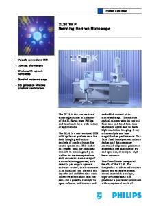
1. INTRODUCTION Scanning Electron Microscopy allows the acquisition of high resolution images of materials using different physical phenomena occuring after the sample is excited by an electron beam [1]. In the case of cementitious materials, BackScattered Electrons (BSE) and X-ray diffraction have been used to obtain two types of images of the tested samples. BSE images are high spatial resolution images (354 nm here) whose gray levels are related to the density of the material at the pixel location, while X-ray images, once the excitation energies are well tuned, can account for the presence of the corresponding chemical elements in the sample. Then a BSE image as well as a collection of X-ray images can be acquired, one for every element to be studied. X-ray images are corrupted by noise and quantization effects occurring during the acquisition. In this case, the width of the images represents around 364 µm of the sample. The data is then a multivariate image of 15 bands in these specific settings (1 for the BSE image, and 14 for the chosen elements, here Al, C, Ca, Cl, Fe, K, Mg, Mn, Na, O, P, S, Si and Ti), as shown in Fig. 1. In the context of cement, the objective is the analysis of the phases present in the sample, in order to monitor the chemical reactions occuring in the cement paste after its solidification, by computing the hydration degree of the components [2]. Thus, to identify the proportions of the phases in a sample, accurate (supervised) classification maps have to be generated. This task can be performed visually by an expert, but there is a need in the cement industry for precision and efficiency achievable with an automation of the procedure, using only training samples identified beforehand (c.f. Fig. 5). Existing classification techniques include multiple thresholding on both types of images [3] [4], decision trees [5], Mean Shift clustering [6], and Support Vector Machines (SVM). The latter can be combined with a spatial regularization based on Markov Random Fields (MRF) in order to exploit the contextual relations of the pixels [7]. The classification maps are spatially more homogeneous, but some structures, such as edges and small objects, which can be significant for estimating the quantity of a material in the sample, are lost. In order to regularize the classification maps, SVMs can also be run on a segmentation of the image, such as a watershed segmentation or a superpixel generation algorithm, such as [8]. In both cases, the information loss due to the regularization is detrimental especially for the fly ashes, i.e. small round or crescent-shaped components that have been more and more used in the cement industry for their beneficial impact on the amount of CO2 rejected in the environment. This paper introduces a

new semi-automatic classification technique based on the denoising of the X-ray images, SVM classification, and interactivity with the user, who will be able to update the training set by integrating new samples by exploiting a segmentation map. The latter is automatically generated using Binary Partition Trees (BPT) but can also be tuned by the user, with the exploration of the tree structure.

Figure 1. A multivariate SEM image of a cement sample.

2. PROPOSED APPROACH The proposed classification method is first based on the denoising of the X-ray bands, necessary to improve the smoothness of the classification maps. Then a hierarchical representation of the regions of the image is generated using a BPT. An automatic pruning of the tree provides a segmentation map to the user, who can improve it by exploring the tree structure. In parallel, an automatic classification is generated using SVMs. The user is then asked to correct some misclassified regions (defined by the segmentation map) that will be then integrated to the training set. The interactivity allowed by the BPT structure is twofold: on a spectral level with the tuning of the training for the classification, and on a spatial level with the exploration of the hierarchical structure of the BPT. A flowchart of the proposed approach is given in Fig. 2. Training Samples

Data

BM3D Denoising

Region Model Merging Criterion Pruning Strategy

BPT Construction

SVM

BPT Pruning

Segmentation map

Classification map

GUI

GUI

Figure 2. Flowchart of the proposed method.

2.1 Denoising The first step is the denoising of the X-ray bands (the BSE band is practically noise free), performed with the BM3D algorithm, first presented in [9]. The variance of the noise, required as the only input parameter, is estimated using Median Absolute Deviation (MAD) [10]. The effect of the denoising on two bands, including one associated to a scarce chemical element which presents strong quantization effects, is shown in Fig. 3, in comparison with a 3 × 3 median filter.

2.2 Interactive Segmentation using BPTs After the denoising step, a segmentation map of the data is generated for the user to be able to interact with the regions of the image. Binary Partition Trees, introduced in [11], are used. BPTs provide a hierarchical tree representation of the regions of the image. Starting from an initial partition (here obtained using a hyperspectral watershed algorithm [12]) with n regions, the two most similar regions are merged to form a new node. The process is repeated iteratively until only one region (the root), whose support is the same as the whole image, is left, forming a tree with 2n−1 nodes. The nodes of the initial partition are called the leaves. An example is shown in Fig. 4. To define a similarity measure between regions, a region model and a merging criterion are required [13,14,15]. For this study, a nonparametric region model was chosen [13]: every region Ri is represented by the set of L histograms {Hl } of the region pixels, one for each of the L available bands: MRi = {H1 , H2 , · · · , HL }. The merging criterion is the so-called diffusion distance, a cross-bin distance between two histograms, adapted to the multivalued case: L X R D(Ri , Rj ) = Dl (HlRi , Hl j ) (1) l=1 R Dl (HlRi , Hl j )

where is the diffusion distance of two histograms as introduced in [16]. Once the tree is built, the following step is to extract a segmentation map by pruning the tree. The idea is to keep a set of nodes that forms a partition of the original image (see Fig. 4 for an example). The simplest pruning strategies consist in a cross-cut of the tree at a given height, or in keeping the partition obtained after a certain number of region mergings. Here, the chosen strategy is to keep one node per branch (a branch is the set of nodes between a leaf and the root) in the final partition, when the Spectral Angle Mapper (SAM) between the chosen region and the sibling region is higher than a given threshold α:   mRi · mRj >α (2) SAM (Ri , Rj ) = arccos ||mRi ||2 × ||mRj ||2 with mRi the mean spectrum of the region pixels. However, the automatic segmentation map cannot be optimal. Small regions may be undersegmented and disappear from the result, while in some other cases, unnecessary partitions are made, e.g. inside the same phase (Fig. 6). However, thanks to the hierarchical structure of the BPT, this automatic segmentation serves as a basis for a user-improved version. To this end, a GUI was implemented to allow the user to explore the tree, starting from the partition defined by the pruning. The current segmentation map is showed next to a representation of the image (e.g. a certain band, a false color composition using PCA, ...). The user is able to display any region (s)he selects and the region corresponding to the parent node. Then (s)he chooses whether or not to perform the merging on oversegmented regions and update the pruning accordingly. Similarly, (s)he may also visualize the two children of a node, and split an undersegmented region if needed. With this simple strategy, the hierarchy defined by the tree helps to refine the already good segmentation results. Typically, only a few corrections are necessary to improve the segmentation map, as can be seen on Fig. 6. Note that this exploration of the image regions remains constrained by the tree structure.

(a) Al X-ray band. (b) 3 × 3 median filter.

(c) BM3D.

(d) Cl X-ray band. (e) 3×3 median filter.

(f) BM3D.

Figure 3. Results of the denoising using the BM3D algorithm on two X-ray bands (Al and Cl) of a cement sample.

(a) An example of the construction of a BPT.

(b) Two possible prunings of the BPT. Only nodes that form a partition of the initial image can be selected.

Figure 4. Illustration of the construction and the pruning of a BPT.

2.3 Interactive Classification using SVMs In parallel with the segmentation step, a classification map is generated using the denoised data, manually defined training samples and multiclass SVMs. The SVM features are simply the pixel values in each band of the image. The denoised data allows the pixelwise SVM classification to be much more homogeneous than with the raw data. However, it is probably not optimal. The most critical parameter in the classification is the definition of the training samples: they have to be good and balanced representatives of the different classes. The idea that motivates our approach is that the user is usually able to spot easily some of the misclassifications (only a few corrections are required in practice). If (s)he could correct a certain part of the classification, the algorithm should be capable of learning from the corrections and adjust the classification map accordingly. The regularization of the classification map is performed on the regions of the segmentation map. Every region of the segmentation map is assigned to the majoritary class among its pixels. Thus, using a second GUI, the user will be able to select the classified regions of the segmentation map. Comparing the classification maps with a representation of the data (e.g. training image, false color composition, ...), the misclassified regions can be easily spotted and assigned to the correct class. The information provided by the user to improve the training samples allows the classifier to learn from the corrections. Based on empirical observations, 5% of the pixels of the chosen regions are randomly selected and added to the training set with a label that corresponds to the corrected class. By repeating this operation on a few misclassified regions, the training set is enriched and becomes more representative of the classes and learns from its previous mistakes. Then a final (pixelwise) SVM classification map is generated from the new training set, using the denoised data as input (the SVM regularization is only useful for the interactive process and is not the final result).

3. VALIDATION

In this section, the results of the proposed classification technique are presented. Fig. 5 shows an example of classification map, compared to the results of SVM on the raw data and the SVM-MRF method of [7]. Visually,

(a) Initial training image and infor- (b) SVM (no denoising). mation on the classes.

(c) SVM-MRF.

(d) Proposed approach.

Figure 5. Classification maps of the proposed method in comparison with SVM and SVM-MRF.

(a) BSE age.

im- (b) First (c) Automatic (d) Corrected (e) SVM with (f) 3 principal segmentation. Segmentation. no denoising. MRF. components.

SVM- (g) SVM on (h) Proposed the denoised Approach. data.

Figure 6. Segmentation (some edges on a fly ash were highlighted) and classification maps of a subset of the image of Fig. 5.

the proposed method, in spite of being pixelwise, provides smooth classification maps because of the denoising, as opposed to SVM. It also preserves the edges of the phases and the smallest regions much more than SVMMRF, which can contribute significantly to the phase percentages, e.g. for the different type of micronized Fly Ashes (FA), often disappearing after the MRF regularization while they are of prime importance for the cement industry. This can be also seen on Fig. 6. In addition, it shows that the SVM on the denoised data is not sufficient in general to guarantee a good separation of the classes, since the denoising step reduces intra-class variability. In this case, the corrected regions mainly added samples for the FA and porosity classes, thus improving their detection rate in the classification maps. For quantitative results, experiments have been performed on one day old cement pastes, at which point we can consider that some of the components have not started to react yet. Then, by comparing the phase percentages on a sufficiently large region to the quantity that was actually put in the cement, the results can be quantified. A full SEM acquisition corresponds to up to 50 tiles of size 1024×768×15. The training and the interactive process was performed on one of these tiles, and the updated training set was then used to perform SVM classifications on every tile, after the denoising step. The phase percentages were then computed on each tile and averaged. A Gaussian Radial Basis Function was used for the SVM kernel. For the MRF, 3 × 3 neighborhoods were used, and XXX XXX Phase XXX Method X BPT SVM-MRF Theory Absolute difference with theory (BPT) Absolute difference with theory (SVM-MRF)

FA in OPC-FA-LF 13.22 16.40 13.90 0.68 2.50

SL in OPC-FA-SL 3.70 3.27 3.97 0.27 0.70

SL in OPC-FA-SL 5.00 6.45 5.84 0.84 0.61

FA in OPC-FA-SL 15.88 12.05 13.92 1.96 1.87

FA in OPC-FA-SL 19.97 19.95 19.10 0.87 0.85

PZN in OPC-PZN 8.25 12.70 7.49 0.76 5.21

FA in OPC-FA 32.84 31.00 31.87 0.97 0.87

Table 1. Phase percentages obtained by the proposed approach (BPT) confronted to those of SVM-MRF. OPC: Ordinary Portland Cement, FA: Fly Ashes, PZ: Pozzolan, SL: Slag, LF: Limestone Fillers. Bold values indicate the best result. Red values indicate better performance for the proposed approach. Blue values indicate comparable performance (absolute error differing by 0.1% or less). The green value correspond to a better performance for SVM-MRF.

Figure 7. Experimental phase percentages plotted against theoretical values for the proposed approach and SVM-MRF.

for the BPT segmentation, a threshold of 0.2 rad was used. The proposed method is compared to the results obtained by SVM-MRF. Quantitative results are given in Table 1 and plotted on Fig. 7. We can see that the BPT approach performs better than SVM-MRF in 3 cases out of 7, comparably in 3 cases out of 7, and worse in only one case. The main improvement can be seen on two cases: FA in a ternary OPC-FA-LF mixture, and PZN in an OPC-PZN mixture (which corresponds to the arrows in Fig 7). The small size of the FA and the complexity of the mixture in the first case and the presence of clay in the second are better handled by the proposed approach. This suggests the potential of the interactive BPT approach as a robust technique for the classification of complex mixtures.

4. CONCLUSION An interactive classification technique for cementitious materials using multivalued SEM images was presented in this paper. It is based on a segmentation step using a BPT, performed after denoising the data, and interactivity with the user. Then a SVM classifier is used, and the user can integrate misclassified regions in the training samples to better represent the classes. The method was compared to another classification approach, both visually and quantitatively using 1-day old cement pastes. The results show the potential of the method for the classification of Fly Ashes, a component of prime importance for the cement industry, as well as complex mixtures. Future work could include inferring decisions from the user’s corrections of the segmentation map to try to learn rules or infer new pruning strategies, and on the classification part an optimal selection of the most informative training samples using the tools of Active Learning.

REFERENCES [1] Goldstein, J., Newbury, D., Joy, D., Lyman, C., Echlin, P., Lifshin, E., Sawyer, L., and Michael, J., [Scanning Electron Microscopy and X-Ray Microanalysis (3 ed) ], Springer (2003). [2] Haha, M. B., de Weerdt, K., and Lothenbach, B., “Quantification of the degree of reaction of fly ash,” Cement and Concrete Research 40, 1620–1629 (2010). [3] Bentz, D. P. and Stutzman, P. E., “Sem analysis and computer modeling of hydration of portland cement particles,” in [Symposium on Petrography of Cementitious Materials ], 60–73 (June 1993). [4] Stutzman, P. E., “Scanning electron microscopy imaging of hydraulic cement microstructure,” Cement and Concrete Composites 26, 957–966 (November 2004). [5] Ding, Q. and Colpan, M., “Decision tree induction on hyper-spectral cement images,” International Journal of Information and Mathematical Science 2(3), 169–175 (2006). [6] Martins, D., Josa, V. G., Castellano, G., and da Costa, J. B., “Phase classification by mean shift clustering of multispectral material images,” Microscopy and Microanalysis 19, 1266–1275 (October 2013). [7] Meulenyzer, S. P., Chanussot, J., Crombez, S., and Chen, J. J., “Spectral spatial image processing strategies for classifying multispectral sem-eds x-ray maps of supplementary cementitious materials,” in [14th Euroseminar on Microscopy Applied to Building Materials], (June 2013). [8] Achanta, R., Shaji, A., Smith, K., Lucchi, A., Fua, P., and Susstrunk, S., “Slic superpixels compared to state-of-the-art superpixel methods,” Pattern Analysis and Machine Intelligence, IEEE Transactions on 34, 2274–2282 (Nov 2012). [9] Dabov, K., Foi, A., Katkovnik, V., and Egiazarian, K., “Image denoising by sparse 3D transform-domain collaborative filtering,” IEEE Transactions on Image Processing 16 (August 2007). [10] Hoaglin, D., Mosteller, F., and Tukey, J., [Understanding robust and exploratory data analysis ], vol. 3, Wiley New York (1983). [11] Salembier, P. and Garrido, L., “Binary partition tree as an efficient representation for image processing, segmentation and information retrieval,” IEEE Transactions on Image Processing 9, 561–576 (April 2000). [12] Tarabalka, Y., Chanussot, J., and Benediktsson, J. A., “Segmentation and classification of hyperspectral images using watershed transformation,” Pattern Recognition 43, 2367–2379 (2010). [13] Valero, S., Salembier, P., and Chanussot, J., “Comparison of merging orders and pruning strategies for binary partition tree in hyperspectral data,” in [Image Processing (ICIP), 2010 17th IEEE International Conference on ], 2565–2568 (Sept 2010).

[14] Valero, S., Salembier, P., and Chanussot, J., “Hyperspectral image representation and processing with binary partition trees,” Image Processing, IEEE Transactions on 22, 1430–1443 (April 2013). [15] Veganzones, M., Tochon, G., Dalla Mura, M., Plaza, A., and Chanussot, J., “Hyperspectral image segmentation using a new spectral mixture-based binary partition tree representation,” in [Image Processing (ICIP), 2013 20th IEEE International Conference on ], 245–249 (Sept 2013). [16] Ling, H. and Okada, K., “Diffusion distance for histogram comparison,” Computer Vision and Pattern Recognition, 2006 IEEE Computer Society Conference 1, 246–253 (June 2006).