Commun. Theor. Phys. (Beijing, China) 36 (2001) pp. 351–356 c International Academic Publishers °

Vol. 36, No. 3, September 15, 2001

Self-organized Criticality in a Model Based on Neural Network∗ ZHAO Xiao-Wei and CHEN Tian-Lun Department of Physics, Nankai University, Tianjin 300071, China

(Received December 6, 2000)

Abstract Based on the LISSOM neural network model, we introduce a model to investigate self-organized criticality in the activity of neural populations. The influence of connection (synapse) between neurons has been adequately considered in this model. It is found to exhibit self-organized criticality (SOC) behavior under appropriate conditions. We also find that the learning process has promotive influence on emergence of SOC behavior. In addition, we analyze the influence of various factors of the model on the SOC behavior, which is characterized by the power-law behavior of the avalanche size distribution. PACS numbers: 64.60.Ht, 87.10.+e

Key words: neuron network, self-organized criticality, avalanche

1 Introduction A few years ago, Bak, Tang and Wiesenfeld introduced the concept of the “self-organized criticality” (SOC) in the sand pile model.[1] From then on, this concept has been widely studied in many extended dissipative dynamical systems, such as earthquake,[2] biology evolution,[3] forest fire,[4] and so on. It is shown that all these large dynamical systems tend to self-organize into a statistically stationary state without intrinsic spatial and temporal scales. This critical state is achieved over a wide range of the parameters of the system and no fine tuning is needed, and it is characterized by a power-law distribution of avalanche sizes, where the size is the total number of toppling events or unstable units. In this sense, the dynamical state of every spatial and temporal scale can emerge if the system is in SOC state. Therefore, it is considered that the system in SOC state has maximal complexity and latent computing potency. The human brain is one of the most complex systems, and it possesses about 1010 ∼ 1012 neurons. The brain’s information process has the properties of stability and variability — on one hand, there is relative stable information stored in the brain; on the other hand, the brain is influenced by the environment and people should continuous update knowledge and points. So it is stated that the brain must operate at the critical state, and it should self-organize to this critical state under some suitable conditions.[5] In fact, the strong analogies between the dynamics of the SOC model for earthquakes and that of neurobiology have been realized by Hopfield.[6] We hope that grasping the mechanics of SOC processes in the brain will be helpful in understanding the higher functions of the brain. So we try to study SOC in the activity of neural populations. Our group has done a work in this area,[7] but it is still immature. In this paper, we introduce a kind of serial cellular automation system which replicates the correlation structure of neural populations, that is, each cell behaves like ∗ The

an integrate-and-fire neuron. The system can emerge SOC behavior in a wide range of system parameters. And more importantly, when the influence of connection (synapse) between neurons is adequately considered, we can find that the model’s learning process, which is important and natural for real brain, plays a promotive role in the emergence of SOC behavior. The work is the first try to study the relation between SOC behavior and the learning process in the brain. In the second section of this paper, a general description of our model is given. In Sec. 3, we show the simulation results of the system and the influence of various factors of the model on the SOC behavior. The conclusion and perspective are contained in the last section.

2 The Model Our model is a kind of serial cellular automaton system based on the LISSOM model.[8] It has two layers, the first one is input layer, there are h neurons, received h-dimensional input vector ζ. The second one is computing layer, it is a two-dimensional square lattice with N × N neurons, and every neuron’s state is ηij . When an h-dimensional vector ζ is inputted, the state ηij (t) of the neuron (i, j) at time t is changed according to the formula nX X µij,h ζh + γe Eij,kl ηkl (t − 1) ηij (t) = σ h

− γi

X k ′ l′

kl

o Iij,k′ l′ ηk′ l′ (t − 1) = σ{fij (t)} ,

(1)

where σ(x) is an active function, and it is a piecewise linear approximation of the familiar sigmoidal activation function,  0, x ≤ 0.6 ,   σ(x) = (x − 0.6)/(1.3 − 0.6) , 0.6 < x < 1.3 , (2)   1, x ≥ 1.3 ;

project supported by National Natural Science Foundation of China under Grant No. 60074020

352

ZHAO Xiao-Wei and CHEN Tian-Lun

µij,h is afferent input weight from an input layer neuron (h) to a computer layer neuron (i, j); Eij,kl is the excitatory lateral connection weight on the connection from the neuron (k, l), which is in the neuron (i, j)’s excitatory lateral connection scope, to the neuron (i, j); I(ij, k ′ l′ ) is the inhibitory connection weight; fij (t) is the local field of the neuron (i, j) at time t; γe and γi are constant factors. According to the dynamic Hebb rule, the adjustment of those three connection weights is as follows: µij,h (t) + αηij ξh µij,h (t + 1) = P , 2 { h [µij,h (t) + αηij ξh ] }1/2 Eij,kl (t) + αE ηij ηkl Eij,kl (t + 1) = P , kl [Eij,kl (t) + αE ηij ηkl ] Iij,k′ l′ (t) + αI ηij ηk′ l′ , (3) k′ l′ [Iij,k′ l′ (t) + αI ηij ηk′ l′ ] where α, αE , αI are the learning rates. Generally, the scope of lateral connection weight is in a local case, and the excitatory lateral connection radius de is smaller than the inhibitory radius di , here we let di = 3de . Note the change of the neuron states is quicker and the adjustment of the connection weights is slower. Usually, after 10 iterations of the neuron states when any pattern is inputted (At this time, the network state becomes an attractor in the state space, often a fixed point), all connection weights are updated once. Thus, after learning a while, the lateral connection weights evolve into the “Mexican hat” profile, the afferent input weights self-organize into a topological map of the input space, and the state of the neural network is evolved from disordered case to stable and topological case in state space. Our system has not some properties of the LISSOM model, such as connection death and modification of activation function σ(x).[8] But, the two models are essentially similar on dynamic behavior, and here we use the same parameters as those in the LISSOM model. Now, we add a kind of integrate-and-fire mechanism into the model for every neuron. The mechanism is to simulate the current neuron-dynamical picture of brain, the essential features of its function are written below.[9] When the membrane potential of a neuron exceeds the threshold, the neuron sends out signals with the form of action potentials and then returns to the rest state (the neuron fires). The signal is transferred by the synapses to the other neurons, which has an excitatory or inhibitory influence on the membrane potential of the receiving cells according to whether the synapses are excitatory or inhibitory, respectively. The resulting potential, if it also exceeds the threshold, leads to the next step firing, and so on giving an avalanche like it in earthquake or sand-pile models. The integrate-and-fire mechanism can be described as follows in detail. Iij,k′ l′ (t + 1) = P

Vol. 36

(i) When the membrane potential fij (t) of neuron (i, j) at time t is below a threshold Vth = 1.3 , we call the neuron (i, j) is stable and it does not influence the others. (ii) If neuron (i, j) is unstable, i.e. fij (t) ≥ 1.3, ηij (t) = 1, it will fire, and each of the nearest four neighbors (i′ , j ′ ) around this unstable neuron will receive a pulse from it. At the same time, the neuron (i, j) becomes stable again, fi′ j ′ → fi′ j ′ + β(Eij,i′ j ′ − Iij,i′ j ′ )ηij , fij → 0 ,

ηij → 0 ,

(4)

here β is a tunable parameter, and the term of β(Eij,i′ j ′ − Iij,i′ j ′ )ηij represents the pulse intensity from an unstable neuron to its neighbors. (iii) Find out the maximal value Vmax , and add Vth − Vmax to all neurons fij → fij + (Vth − Vmax ) .

(5)

This driving process represents that all the neurons receive continual driving from external or other parts of the brain. At the same time we must make all fij > 0. Now, we present the computer simulation procedure of this model in detail, here we have used open boundary condition. (a) Variable initialization In the two-dimensional n × n lattice, let the initiatory state and local field equal 0; randomly initialize each connection weight among [0, 1]; and keep the total excitatory (inhibitory) lateral connection weights of every neuron be constant (It is 1). The random input patterns ζj (j = 1, 2, 3) are produced according to ζ1 = 1 × cos x1 cos x2 , ζ2 = 1 × sin x1 cos x2 ,

ζ3 = 1 × sin x2 ,

where x1 , x2 are random numbers between [−0.5, 0.5]. It is the same as input vector of the LISSOM model.[8] (b) Learning process We input patterns randomly, iterate the neuron state and local fields according to formula (1), and adjust the three connection weights according to formula (3). After a period of time, the state of the network reaches stability and we consider that the map of input patterns has been stored. (c) Associative memory and avalanche process Input a new pattern, then search the unstable neuron (i, j) as defined above in whole lattice. If there exits any unstable neuron (i, j): fij ≥ 1.3, ηij = 1, redistribute the states of it and its nearest neighbors according to Eq. (4). Repeat this procedure until all the neurons of the lattice are stable. Define this process as one avalanche, and define the avalanche size as the number of all unstable neurons in this process. Then begin drive process (iii) by formula (5), another avalanche begins. In fact, the integrate-and-fire mechanism is similar with the dynamical rule of the earthquake model,[2] but

No. 3

Self-organized Criticality in a Model Based on Neural Network

there is important difference between them. In our mechanism, we adequately consider the influence of lateral connection weight between neurons.

3 Simulation Results 3.1 Power-Law Behavior and Influence of Learning Process First, we let the size of lattice be 20 × 20, β = 21, and make the excitatory lateral connection radius de = 3, the inhibitory connection radius di = 3de . Here, we consider two situations, one is without learning process, the other is learning 3000 times. These two situations can be seen in Fig. 1. We find that in associated with memory process, for learning situation, the distribution

353

of the avalanche size satisfies the power-law behavior P (S) ∝ S −τ , τ ≈ 1.29. We can also see, for without learning situation, the power-law is not obvious as before (learning situation), and P (S) deviates from power-law more and more in large size S, the probability of large scale avalanches is smaller than before. Why does this phenomenon happen? We think that it is the influence of lateral connection weights. To check our idea, we draw the lateral connections of a neuron sited at position (11, 11) in Fig. 2. It can be clearly seen that the excitation and inhibition weights are randomly distributed before learning (Fig. 2a), and a very smooth “Mexican hat” profile evolves around this neuron (11, 11) well after learning 3000 times (Fig. 2b). The result is similar to the case of the LISSOM model.[8]

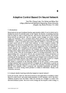
Fig. 1 The probability of the avalanche size (unstable neurons) P (S) as a function of size S for a 20 × 20 system with the lateral connections di = 3de = 9, β = 21. The curves correspond to two conditions: one is with learning 3000 times, another is without learning process.

Fig. 2 The combined lateral interaction of lateral excitation and inhibition weights for a neuron sited at position (11, 11) in the 20 × 20 system. (a) Before learning process. (b) After learning process.

354

ZHAO Xiao-Wei and CHEN Tian-Lun

Without learning process, the lateral connection between fire (unstable) neuron and its neighbors may be very small, even negative, so the term β(Eij,i′ j ′ − Iij,i′ j ′ )ηij may be very small even negative. On the other hand, with learning condition, the lateral connections between neurons self-organize into smooth “Mexican hat” profile, so the pulse intensity between fire (unstable) neuron and its neighbors is stronger than previous (without learning process) condition. We can see in the next subsection, with the pulse intensity decrement, the probability of large scale avalanche will decrease, the result is similar to the result of Refs [7] and [10]. Because the brain is a kind of neural network and synapse weight learning process is important for information process of the brain, the adding of learning process and lateral connection between neurons in our system is very natural. At the same time we find that the SOC behavior in learning condition is better than that without learning condition. It can be thought that, before learning, the system operates at a sub-critical state, in which case the external input signal can only access to a small,

Vol. 36

limited part of the system. After learning process, the system is trained to operate at the SOC state, which is highly sensitive to small outer inputs and robust. It is consistent with P. Bak’s view — the brain can be neither sub-critical nor super-critical, it must be critical and self-organized.[5] So for further investigation, we use the condition with learning process below. 3.2 Influence of the Pulse Discharging Intensity Parameter β In the avalanche process, the influence of parameter β of Eq. (4) is very important. As shown in Fig. 3a, when β is small, the probability of the avalanche size P (S) decays exponentially with the size of the avalanches, which means that there are only localized behaviors. With β increasing, the power-law behavior gradually generates, and the transition from localization to SOC behavior occurs. From Fig. 3b, we can see that the critical exponent τ depends on β. The exponent τ decreases with the increment of β. It is similar to the results of OFC model[2] and Ref. [7].

Fig. 3 (a) The same as Fig. 1, but with pulse discharging intensity parameter β changed. (b) The power-law exponent τ as a function of pulse discharging intensity parameter β.

No. 3

Self-organized Criticality in a Model Based on Neural Network

355

Fig. 4 The avalanche average size hSi as a function of the pulse intensity parameter β for a 20 × 20 system, another parameters are the same as those in Fig. 1.

At the same time, we investigate the relation between the avalanche average size hSi and parameter β. From Fig. 4, we can see that with the increment of β, hSi also increases, and at last, the slope of the curve becomes quite large. This is consistent with the results in Ref. [11], where the mean avalanche size increases extremely quick as the system’s conservative limit is approached (dissipation tends to zero). 3.3 Influence of Lattice Size In the OFC model, the lattice size N is important. We have investigated the influence of lattice size too. In Fig. 5, we show the results of simulations with N = 10, 20, 30. Here we can see that, with the increment of size N , the range of SOC behavior increases too, the cutoff in the avalanche distribution scales with the system size N . It is a kind of finite-size effect and similar to the results of OFC earthquake model.[2]

Fig. 5 Simulation results for the probability of the avalanche size P (S) as a function of size S with di = 3, de = 9, β = 20. The different curves refer to different system sizes, N = 10, 20, 30.

4 Conclusion and Discussion In conclusion, based on the LISSOM neural network model, we have introduced a cellular automaton model which adequately considers the connections of neurons and

replicates the correlation structure of neural populations. Our model can emerge SOC behavior in a wide range of the system parameters. More importantly, we find that the learning process has promotive influence on SOC be-

356

ZHAO Xiao-Wei and CHEN Tian-Lun

Vol. 36

havior and this process is natural in our model. In addition we have analyzed the influence of various factors of the model. Our work just tries to indicate some relations between SOC behavior and brain dynamical process. It might provide an approach for analyzing the collective behavior of neuron populations in brain. Based on SOC behavior, maybe we can describe the information process of the brain as follows. When an outer pattern (external sig-

nal) is inputted into the brain, after learning process, the brain is trained to operate at the SOC state, the neuron populations in the brain behave SOC behavior, the pattern is stored in the brain as an SOC attractor, and the associative memory can be designed as the process of the input pattern evolving into the attractor. But our model is only a very simple simulation of the brain and many details of neurobiology are ignored, so there are still a lot of work to be done.

References

[6] John J. Hopfield, Phys. Today 47 (1994) 40. [7] HUANG Jing and CHEN Tian-Lun, Commun. Theor. Phys. (Beijing, China) 33 (2000) 365. [8] J. Sirosh and R. Miikkulainen, Biol. Cybern. 71 (1994) 65. [9] Dan-Mei CHEN, et al., J. Phys. A: Math. Gen. 28 (1995) 5177. [10] S. Lise and H.J. Jense, Phys. Rev. Lett. 76 (1996) 2326.

[1] P. Bak, C. Tang and K. Wiesenfield, Phys. Rev. A38 (1988) 364. [2] Z. Olami, S. Feder and K. Christensen, Phys. Rev. Lett. 68 (1992) 1244. [3] P. Bak and K. Sneppen, Phys. Rev. Lett. 71 (1993) 4083. [4] K. Christensen, H. Flyvbjerg and Z. Olami, Phys. Rev. Lett. 71 (1993) 2737. [5] P. Bak, How Nature Works: the Science of Self-organized Criticality, Springer-Verlag Press, New York (1996).

[11] M.L. Chabanol and V. Hakim, Phys. Rev. E56 (1997) R2343.