Selective Perception Policies for Guiding Sensing and Computation in Multimodal Systems: A Comparative Analysis Nuria Oliver a,∗ Eric Horvitz a a Adaptive

Systems & Interaction, Microsoft Research, Redmond, WA

Corresponding author Nuria Oliver Adaptive Systems & Interaction, Microsoft Research, Redmond, WA 98052 Phone: +1 425 705 4051 Fax: +1 425 936 7329 Email: [email protected]

∗ Corresponding author. Email addresses: [email protected] (Nuria Oliver), [email protected] (Eric Horvitz). URL: http://research.microsoft.com/∼nuria (Nuria Oliver).

Preprint submitted to Elsevier Science

8 December 2003

Abstract Intensive computations required for sensing and processing perceptual information can impose significant burdens on personal computer systems. We explore several policies for selective perception in SEER, a multimodal system for recognizing office activity that relies on a layered Hidden Markov Model representation. We review our efforts to employ expected-value-of-information (EVI) computations to limit sensing and analysis in a context-sensitive manner. We discuss an implementation of a one-step myopic EVI analysis and compare the results of using the myopic EVI with a heuristic sensing policy that makes observations at different frequencies. Both policies are then compared to a random perception policy, where sensors are selected at random. Finally, we discuss the sensitivity of ideal perceptual actions to preferences encoded in utility models about information value and the cost of sensing. Key words: Selective perception, expected value of information, automatic feature selection, Hidden Markov models, office awareness, multi-modal interaction, human behavior recognition

1

Introduction

Investigators have long been interested in the promise of performing automatic recognition of human behavior and intentions from observations. Successful recognition of human behavior enables compelling applications, including automated visual surveillance and multimodal human–computer interaction (HCI)—considering multiple streams of information about a user’s behavior and the overall context of a situation to provide appropriate control and services. There has been progress on multiple fronts in recognizing human behavior and intentions. However, challenges remain for developing machinery that can provide rich, human-centric notions of context in a tractable manner. We address in this paper the computational burden associated with perceptual analysis. Computation for visual and acoustical analyses has typically required a large portion –if not nearly all– of the total computational resources of personal computers that make use of such perceptual inferences. It is not surprising to find that there is little interest in invoking such perceptual services when they require a substantial portion of the available CPU time, significantly slowing down more primary applications that are supported or extended by the perceptual apparatus. Thus, we have pursued coherent strategies for automatically limiting in an automated manner the computational load of perceptual systems. 2

Our work centers on the control of perception in SEER, a probabilistic reasoning system that provides real-time interpretations of human activity in and around an office [1]. We have explored two strategies for sensor selection and sensor data processing in SEER. The first approach is based on the use of decision-theoretic principles to guide perception, where we compute the expected value of information (EVI) of different subsets of observations in real-time on a frame by frame basis. This is a greedy, one-step lookahead approach to computing the next best set of observations to evaluate at each time step. We refer to this strategy as EVI-based perception. The second approach to limiting the computational burden of perception centers on defining heuristically policies by specifying observational frequencies and duty cycles with which each feature extracted from the sensors is computed. We name this approach rate-based perception. We will compare the performance of the EVI-based and the rate-based perception methods with the legacy SEER system that analyzes all features all the time (i.e. without selective perception), and with a random feature selection perception approach, where the features are randomly selected at each time step. This paper is organized as follows: We first provide background on contextsensing systems and principles for guiding perception in Section 2. In Section 3 we describe the challenge of understanding human activity in an office setting and review the different perceptual inputs that are used. We also provide background on the legacy SEER system, focusing on our work to extend a single-layer implementation of HMMs into a more effective cascade of HMMs, a representation that we refer to as Layered Hidden Markov Models (LHMMs). Section 4 describes the three selective perception strategies that we have developed: EVI-based, rate-based and random-based perception. In Section 5 we review the implementation of a new version of the SEER system that we refer to as Selective SEER (S-SEER hereafter). Experimental results with the use of S-SEER are presented in Section 6. Finally, we summarize our work and highlight several future research directions in Section 7.

2

Prior Related Work

Human Activity Recognition Most of the prior work on leveraging perceptual information to recognize human activities has centered on the identification of a specific type of activity in a particular scenario. Many of these techniques are targeted at recognizing single, simple events, e.g., “waving the hand” or “sitting on a chair”. 3

Only in recent years more effort has been applied to research on methods for identifying more complex patterns of human behavior, extending over longer periods of time. A significant portion of work in this arena has harnessed Hidden Markov Models (HMMs) [2] and extensions. Starner and Pentland in [3] use HMMs for recognizing hand movements used to relay symbols in American Sign Language. More complex models, such as Parameterized-HMMs [4], Entropic-HMMs [5], Variable-length HMMs [6], Coupled-HMMs [7], structured HMMs [8] and context-free grammars [9] have been used to recognize more complex activities such as the interaction between two people or cars on a freeway. Moving beyond the independence assumptions made by HMMs, over the last several years more general dependency models, represented as dynamic Bayesian networks have been adopted for the modeling and recognition of human activities [10–15]. Finally, beyond recognizing specific gestures or patterns the dynamic Bayesian network models have been used to make inferences about the overall context of the situation of people. Recent work on probabilistic models for reasoning about a user’s location, intentions, and focus of attention have highlighted opportunities for building new kinds of applications and services [16]. We have explored the use of a layering of probabilistic models at different levels of temporal abstraction. We have shown that this representation allows a system to learn and recognize in real-time common situations in office settings [1]. Although the methods have performed well, a great deal of perceptual processing has been required by the system, consuming most of the resources available by personal computers. We have thus been motivated to explore strategies for selecting on-the-fly the most informative features, starting with the integration of decision-theoretic approaches to information value for guiding perception.

Principles for Guiding Perception Decision theory studies mathematical techniques for deciding between alternative courses of action. It provides an overall mathematical framework for reasoning about the net value of information [17]. Expected value of information (EVI) refers to the expected value of making observations under uncertainty, taking into consideration the probability distribution over values that will be seen should an observation be made. The connection between decision theory and perception received some attention by AI researchers studying computer vision tasks in the mid-70’s, but interest faded for nearly a decade. Decision theory was used to model the behavior of vision modules [18], to score plans of perceptual actions [19] and 4

plans involving physical manipulation with the option of performing simple visual tests [20]. This early work introduced decision-theoretic techniques to the perceptual computing community. Following this early research, was a second wave of interest in applying decision theory in perceptual applications in the early 90’s, largely for computer vision systems [21] and in particular in the area of active vision search tasks [22].

3

Toward Robust Context Sensing

Before focusing on the control of perceptual actions, we will discuss in more detail the domain and original SEER office-awareness prototype. We will turn to selective perception in Section 4. A key challenge in inferring human-centric notions of context from multiple sensors is the fusion of low-level streams of raw sensor data—for example, acoustic and visual cues—into higher-level assessments of activity. We have developed a probabilistic representation based on a tiered formulation of dynamic graphical models that we refer to as Layered Hidden Markov Models (LHMMs) [1]. For recognizing office situations, we have explored the challenge of fusing information from the following sensors: 1. Binaural microphones: Two mini-microphones (20 − 16000 Hz, SNR 58 dB) capture ambient audio information and are used for sound classification and localization. The audio signal is sampled at 44100 KHz. 2. Camera: A video signal is obtained via a standard Firewire camera, sampled at 30 f.p.s, that is used to determine the number of persons present in the scene. 3. Keyboard and mouse: We keep a history of keyboard and mouse activities during the past 1, 5 and 60 seconds. 3.1 Hidden Markov Models (HMMs) In early work on SEER we explored the use of single-layer hidden Markov models (HMMs) to reason about an overall office situation. Graphically, HMMs are often depicted “rolled-out in time”, as displayed in Figure 1 (a). We found that a single-layer HMM approach generated a large parameter space, requiring substantial amounts of training data for a particular office or user. The single-layer model did not perform well: the typical classification accuracies were not high enough for a real application. Also, when the system was moved 5

to a new office, copious retraining was typically necessary to adapt the model to the specifics of the signals and/or user in the new setting. Thus, we sought a representation that would be robust to typical variations within office environments, such as changes of lighting and acoustics, and models that would allow the system to perform well when transferred to new office spaces with minimal tuning through retraining.

Fig. 1. Graphical representation of (a) HMMs, and (b) LHMMs with 3 different levels of temporal granularity.

3.2 Layered Hidden Markov Models (LHMMs) We converged on the use of a multilayer representation that reasons in parallel at multiple temporal granularities, by capturing different levels of temporal detail. We formulated a layered HMM (LHMM) representation that had the ability to decompose the parameter space in a manner that reduced the training and tuning requirements. In LHMMs, each layer of the architecture is connected to the next layer via its inferential results. The representation segments the problem into distinct layers that operate at different temporal granularities 1 —allowing for temporal abstractions from pointwise observations at particular times into explanations over varying temporal intervals. LHMMs can be regarded as a cascade of HMMs. The structure of a three-layer LHMM is displayed in Figure 1 (b). The layered formulation of LHMMs makes it feasible to decouple different levels of analysis for training and inference. As we review in [1], each level of 1

The “time granularity” in this context corresponds to the window size or vector length of the observation sequences in the HMMs.

6

the hierarchy is trained independently, with different feature vectors and time granularities. In consequence, the lowest, signal-analysis layer, that is most sensitive to variations in the environment, can be retrained, while leaving the higher-level layers unchanged. Figure 1(b) highlights how we decompose the problem into layers with increasing time granularity.

4

Selective Perception Policies

Although the legacy SEER system performs well, it consumes a large portion of the available CPU time to process video and audio sensor information to make inferences. We integrated into SEER several methods for selecting features dynamically: EVI-based perception, based on calculations of the Expected Value of Information (EVI); and rate-based perception, an observational frequency approach. In experiments, we studied the performance of the system using these methods as compared with the legacy SEER system, and with a random perception approach, where features are randomly selected, frame by frame.

4.1 EVI for Selective Perception We focused our efforts on implementing a principled, decision-theoretic approach for guiding perception. Thus, we worked to apply expected value of information (EVI) to determine dynamically which features to extract from sensors in different contexts. EVI policies for guiding sensing and computational analysis of sensory information promised to endow SEER with an ability to limit computation with utility-directed information gathering. The following properties of SEER and its problem domain are conductive to implementing an EVI analysis: (1) a decision model is available that allows the system to make decisions with incomplete information; (2) the decision model can be used to determine the value of information for different sets of variables used in the decision; (3) there are multiple information sources, associated with different costs and response times; (4) the system operates in a personal computing environment with limited resources (CPU, time): gathering all the relevant information all the time before making the decision is very expensive. A critical issue is deciding which information to collect when there is a cost associated with its collection. We compute the expected value of information for a perceptual system by considering the value of eliminating uncertainty about the state of the set of features fk , k = 1...K, under consideration. For example, the features associated with the vision sensor (camera) are motion 7

density, face density, foreground density and skin color density in the image. There are K = 16 possible combinations of these features and we wish the system to determine in real-time which combination of features to compute, depending on the context 2 .

Perceptual Decisions Grounded in Models of Utility We wish to guide the sensing actions with a consideration of their influence on the global expected utility of the system’s performance under uncertainty. Thus, we need to endow the perceptual system with knowledge about the value of action in the world. In our initial work, we encoded utility as the cost of misdiagnosis by the system. We assess utilities, U (Mi , Mj ), as the value of asserting that the real-world activity Mi is Mj . In any context, a maximal utility is associated with the accurate assessment of Mj as Mj . Uncertainty About the Outcome of Observations Let us take fkm , m = 1...M to denote all possible values of the feature combination fk , and E to refer to all previous observational evidence. The expected value (EV) of computing the feature combination fk is, EV (fk ) =

X

P (fkm |E) max i

m

X

P (Mj |E, fkm )U (Mi , Mj )

(1)

j

As we are uncertain about the value that the system will observe when it evaluates fk , we consider the change in expected value associated with the system’s overall output, given the current probability distribution of the different values m that would be obtained if the features in fk would in fact be computed, P (fkm |E). The expected value (EVI) of evaluating a feature combination fk is the difference between the expected utility of the system’s best action when observing the features in fk and not observing them, minus the cost of sensing and computing such features, cost(fk ). If the net expected value is positive, then it is worth collecting the information and therefore computing the features. EV I(fk ) = EV (fk ) − max i

X

P (Mj |E)U (Mi , Mj ) − cost(fk )

(2)

j

2

In the following we will refer to features instead of sensors, because one can compute different features for each sensor input –e.g. skin density, face density, motion density, etc, for the camera sensor.

8

where cost(fk ) is in our case the computational cost associated with computing feature combination fk . Perceptual systems normally incur significant cost with the computation of the features from the sensors. Thus, we trade the information value of observations with the cost due to the analysis required to make the observations. Note that all the terms in Equation 2 should have the same units. Traditionally, EVI approaches convert all the terms to dollars. In our case, we use a scale factor for the cost(fk ). Just as we can acquire detailed preferences about the value model, we can assess preferences about the cost of computation in different settings. The cost can be represented by a rich model that that continues to take into consideration changes in the usage context. For a system like SEER, which was designed to run in the background, monitoring the user’s daily activities in the office, the cost of computation is significant when a user is engaged in a resource-intensive primary computing task and is insignificant when the user is not using the computer. Thus, as we show in Section 6.2, we can construct an expected cost model that takes into consideration the likelihood that a user will experience poor responsiveness because of the portion of CPU that is being used by SEER.

Single and Multistep Analyses For tractability, real-world applications of EVI typically employ a greedy approach, computing the next best observations at each step, making a false assumption that the final system action will occur in the next step. Although we similarly use a greedy strategy to compute the next best observations, we extend typical EVI computations by reasoning about different combinations of features, fk . In our analysis, the system selects the feature combination with the greatest EVI, i.e. f ∗ = arg maxk EV I(fk ). As indicated by Equation 1, the computation of EVI, even in the case of greedy analysis, requires for each piece of unobserved evidence, probabilistic inference about the outcome of seeing the spectrum of alternate values should that observation be computed. Thus, even one-step lookaheads can be computationally costly. A variety of less-expensive approximations for EVI have been explored [23,24]. As we show next, we exploit dynamic programming in HMMs to achieve an efficient algorithm to determine the EVI associated with each feature combination. We follow an approach similar to other architectures, referred to as sequential diagnosis, for interleaving the computation of beliefs and executing information acquisition [25,26,24,27]; we embed the graphical model framework in an architecture with two interconnected modules: the first module (probabilistic module) specifies a graphical model and its associated algorithms for comput9

ing probabilities and processing evidence. The second module (control module) incorporates the method for selective gathering of evidence. Both modules cooperate such that the control module queries the probabilistic module for information about the variables of interest and decides on what computations should be performed next by the probabilistic module.

EVI in HMMs Our probabilistic modules are HMMs, with one HMM per class. In the case of HMMs, with continuous observation sequences {O1 , ..., Ot , Ot+1 }, the term P (fkm |E) from Equation 1 is given by: P (fkm |E) =

X

fm

k |Mn )P (Mn ) p(Ot+1

(3)

n

∝

XX X fkm [ αtn (s) ansl bnl (Ot+1 )]P (Mn ) n

s

l

where αtn (s) is the alpha or forward variable at time t and state s in the standard Baum-Welch algorithm [28], ansl is the transition probability of going fkm fkm ) is the probability of observing Ot+1 in from state s to state l, and bnl (Ot+1 state l, all of them in model Mn . Therefore the EVI of features fk is given by 3 :

EV I(fk ) =

Z

fk ) max p(Ot+1 i

− max i

X

X j

U (Mi , Mj )p(Mj )dOfk

t+1

fk ) U (Mi , Mj )p(Mj ) − cost(Ot+1

j

Z XX X fk ∝ )]P (Mn ) [ αtn (s) ansl bnl (Ot+1 n

max i

s

X j

− max i

l

U (Mi , Mj )p(Mj )dOfk

(4)

t+1

X

fk ) U (Mi , Mj )p(Mj ) − cost(Ot+1

j

If we discretize the observation space into M bins 4 , Equation 4 becomes: 3

For the sake of conciseness, we will drop hereafter the conditioning on the previous evidence, E (observations in the HMMs case {O1 ...Ot }). 4 In S-SEER M is typically 10.

10

M XX X X fkm )]P (Mn ) ansl bnl (Ot+1 [ αtn (s) EV I ∝ m=1 n

max i

X j

− max i

s

l

U (Mi , Mj )p(Mj )

X

fk U (Mi , Mj )p(Mj ) − cost(Ot+1 )

(5)

j

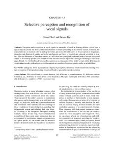
The computational overhead added to carry out the EVI analysis is –in the discrete case– O(M ∗ F ∗ N 2 ∗ J), where M is the maximum cardinality of the features, F is the number of feature combinations, N is the maximum number of states in the HMMs and J is the number of HMMs. 4.2 Heuristic Rate-based Perception In order to better understand the properties of the EVI approach, we have developed alternative methods for selective perception. We explored, in a second selective perception policy, a heuristic, rate-based approach. This policy consists of defining an observational frequency and duty cycle (i.e. amount of time during which the feature is computed) for each feature f . Figure 2 illustrates an example of different observational frequencies and duty cycles for four features: audio classification, video classification (person presence), sound localization and keyboard and mouse activities. With this approach, each feature f is computed periodically. The period between observations and the duty cycle of the observation is determined by means of cross-validation on a validation set of real-time data. The rationale behind this rate-based perception strategy is based on the observation that not all the features are needed all the time: the system should be able to make accurate inferences about the current activity with partial information about the current state of the world. For example, to identify that a Presentation is taking place, the system heavily relies on the keyboard and mouse activities and on the audio classification. The video classification and sound localization features become less relevant. Therefore, instead of computing all the features all the time, one could set a high frequency for the computation of the audio and keyboard/mouse features, and a low frequency for computing the video and sound localization. Because HMMs process the data contained in a sliding window of length T , their inferences are robust to some missing (non-observed) features in some of the data points of the sliding window.

11

Period ON Video Classification OFF Duty Cycle

ON

Audio Classification OFF

ON Sound Localization OFF

ON Keyboard & Mouse OFF

Fig. 2. Example of observational frequencies and duty cycles for four features: audio classification, video classification, sound localization and keyboard and mouse activities.

Although we defined a heuristic rate-based policy, we note that a rate-based formulation could be used within an EVI framework. That is, observational rates and duty cycles for sensors can serve as control parameters optimized with an EVI analysis at design time or in real-time. We are investigating the development of an EVI-mediated, rate-based system.

4.3 Random Selection For another baseline policy, we developed a simple random-selection method, where features are selected randomly for use on a frame-by-frame basis. In this case, the average computational cost of the system is constant, independent of the current sensed activity, and lower than the cost of computing all of the features all the time.

5

Implementation of S-SEER

S-SEER operates the same way as its predecessor, SEER, except in the avail-

ability of several selection perception policies. For clarity, we shall include a brief summary of the core system and move onto the details of experiments with selective perception in Section 6.

5.1 Core Learning and Inference SEER consists of a two-level LHMM architecture with three processing layers. For a more detailed description we direct the reader to [1]. 12

Feature Extraction in S-SEER The raw sensor signals are preprocessed in S-SEER to obtain feature vectors (i.e. observations) for the first layer of HMMs. With respect to the audio analysis, Linear Predictive Coding coefficients [2] are computed. Feature selection is applied to these coefficients via principal component analysis. The number of features is selected such that at least 95% of the variability in the data is maintained, which is typically achieved with no more than 7 features. We also extract other higher-level features from the audio signal such as its energy, the mean and variance of the fundamental frequency over a time window, and the zero crossing rate [2]. The source of the sound is localized using the Time Delay of Arrival (TDOA) method. Four features are extracted from the video signal: the density of skin color in the image (obtained by discriminating between skin and non-skin models, consisting of histograms in YUV color space), the density of motion in the image (obtained by image differences), the density of foreground pixels in the image (obtained by background subtraction, after having learned the background), and the density of face pixels in the image (obtained by means of a real-time face detector [29]). Finally, a history of the last 1, 5 and 60 seconds of mouse and keyboard activities is logged.

First Level HMMs The first level of HMMs includes two banks of distinct HMMs for classifying the audio and video feature vectors. The structure for each of these HMMs is determined by means of cross-validation on a validation set of real-time data. On the audio side, we train one HMM for each of the following office sounds: human speech, music, silence, ambient noise, phone ringing, and the sounds of keyboard typing. In our architecture, all the HMMs are run in parallel. At each instant, the model with the highest likelihood is selected and the data –e.g. sound in the case of the audio HMMs– is classified correspondingly. We will refer to this kind of HMMs as discriminative HMMs. The video signals are classified using another bank of discriminative HMMs that implement a person detector. At this level, the system detects whether nobody, one person (semi-static), one active person, or multiple people are present in the office. Each bank of HMMs can use any of the previously defined selective perception strategies to determine which features to use. For example, a typical scenario is one where the system uses EVI analysis to select in real-time the motion and skin density features when there is one active person in the office, and skin density and face detection when there are multiple people present. 13

Second Level HMMs The inferential results 5 from this layer (i.e. the outputs of the audio and video classifiers), the derivative of the sound localization component, and the history of keyboard and mouse activities constitute a feature vector that is passed to the next (third) and highest layer of analysis. This layer handles concepts with longer temporal extent. Such concepts include the user’s typical activities in or near an office. In particular, the activities modeled are: (1) Phone conversation; (2) Presentation; (3) Face-to-face conversation; (4) User present, engaged in some other activity; (5) Distant conversation (outside the field of view); (6) Nobody present. Some of these activities can be used in a

variety of ways in services, such as those that identify a person’s availability. The models at this level are also discriminative HMMs and they can also use selective perception policies to determine which inputs from the previous layer to use.

5.2 Performance of SEER We have tested S-SEER in multiple offices, with different users and respective environments for several weeks. In our tests, we have found that the high-level layers of S-SEER are relatively robust to changes in the environment. In all the cases, when we moved S-SEER from one office to another, we obtained nearly perfect performance without the need for retraining the higher levels of the hierarchy. Only some of the lowest-level models required re-training to tune their parameters to the new conditions (such as different ambient noise, background image, and illumination) . The fundamental decomposability of the learning and inference of LHMMs makes it possible to reuse prior training of the higher-level models, allowing for the selective retraining of layers that are less robust to the variations present in different instances of similar environments.

5.3 HMMs vs LHMMs In a more quantitative study, we compared first the performance of our model with that of single, standard HMMs. The feature vector in the latter case results from the concatenation of the audio, video and keyboard/mouse activities features in one long feature vector. We refer to these HMMs as the Cartesian Product (CP) HMMs. 5

See [1] for a detailed description of how we use these inferential results.

14

Note that the number of parameters to estimate is much lower for LHMMs than for CP HMMs. Moreover, in LHMMs the inputs at each level have already been filtered by the previous level and are more stable than the feature vectors directly extracted from the raw sensor data. Therefore, encoding prior knowledge about the problem in the structure of the models decomposes the problem in a set simpler subproblems and reduces the dimensionality of the overall model. For the same amount of training data, we would expect LHMMs to have superior performance than HMMs. Our experimental results corroborate this expectation. We direct the reader to [1] for a detailed description of the experiments comparing HMMs and LHMMs for office activity recognition as well as to a detailed review of an evaluation of the recognition accuracy of the system.

6

Experiments with Selective Perception

We performed a comparative evaluation of the S-SEER system when executing the EVI, rate-based, and random selective perception algorithms.

6.1 Studies of Accuracy and Computation In an initial set of studies, we considered diagnostic accuracy and the computational cost incurred by the system. The results are displayed in Tables 1, 2 and 3, and in Figure 3. We use the abbreviations: PC=Phone Conversation; FFC=Face to Face Conversation; P=Presentation; O=Other Activity; NP=Nobody Present; DC=Distant Conversation. Figure 3 illustrates the automatic toggling on and off of features when running the EVI analysis in S-SEER in the office and switching between different activities. The figure shows only the transitions among activities. If a feature was turned on, its activation value in the graph is 1 whereas it is 0 if it was turned off. The vertical lines indicate the change of activity and the labels on the top show which activity was taking place at that moment. In this experiments we assume a simple utility model represented as the identity matrix. Observations that can be noted from the figure include: (1) At times the system does not use any features at all. For example at time=50, no features are evaluated as the system is confident enough about the situation, and it selectively turns the features on only when necessary; (2) the system guided by EVI tends to have longer switching time (i.e. the time that it takes to the system to realize that a new activity is taking place) than when using all the features all the time. We found that the EVI computations trigger the 15

Fig. 3. Automatic selection of features when transitioning between different office activities. Each graph represents the activation of one feature: video processing, audio processing, sound localization and computer activity monitoring.

use of features again only after the likelihoods of hypotheses have sufficiently decreased, i.e. none of the models is a good explanation of the data; (3) in the example, the system never turns the sound localization feature on, due to its high computational cost versus the relatively low informational value the acoustical analysis provides. Tables 1 and 2 compare the average recognition accuracy and average computational cost (measured as % of CPU usage) when testing S-SEER on 600 sequences of office activity (100 sequences/activity) with and without (first column, labeled “Nothing”) selective perception. Note how S-SEER with selective perception achieved as high a level of accuracy as when evaluating all the features all the time, but with a significant reduction on the CPU usage. These results correspond to the following observational rates (in seconds): 10 for the audio channel, 20 for the video channel, .03 for the keyboard and mouse activities and 20 for the sound localization. The recognition accuracy for Phone Conversation in the rate-based approach is much lower than for any of the other activities. This is because the system needs to use video information more often than every 20 seconds in order to appropriately recognize that a Phone Conversation is taking place. If we raise the rate of using video to 10 seconds, while keeping the same observational frequencies for the other sensors, the recognition accuracy for Phone Conversation becomes 89%, with a computational cost of 43%. 16

Table 1 Average accuracies for S-SEER with and without different selective perception strategies. Recognition Accuracy (%) Nothing

EVI

Rate-based

Random

PC

100

100

29.7

78

FFC

100

100

86.9

90.2

P

100

97.8

100

91.2

O

100

100

100

96.7

NP

100

98.9

100

100

DC

100

100

100

100

Table 2 Average computational costs for S-SEER with and without different selective perception strategies. Computational Costs (% of CPU time) Nothing

EVI

Rate-based

Random

PC

61.22

44.5

37.7

47.5

FFC

67.07

56.5

38.5

53.4

P

49.80

20.88

35.9

53.3

O

59

19.6

37.8

48.9

NP

44.33

35.7

39.4

41.9

DC

44.54

23.27

33.9

46.1

6.2 Richer Utility and Cost Models The EVI-based approach experiments previously reported correspond to using an identity matrix as the system’s utility model U (Mi , Mj ) and a measure of cost cost(fk ), proportional to the percentage of CPU usage. However, we can assess more detailed models that capture a user’s preferences about different misdiagnoses in various usage contexts and about latencies associated with computation for perception. Models of the Cost of Misdiagnosis As an example, one can assess in dollars the cost to a user of misclassifying Mi as Mj , i, j = 1...N in a specific setting. In one assessment technique, for each actual office activity Mi , we seek the dollar amounts that users would 17

be willing to pay to avoid having the activity misdiagnosed as Mj by an automated system, for all N − 1 possible misdiagnoses. Models of the Cost of Perceptual Analysis In determining a real world measure of the expected value of computation, we also need to consider the deeper semantics of the computational costs associated with perceptual analysis. To make cost-benefit tradeoffs, we map the computational cost and the utility to the same currency. Thus, we can assess cost in terms of dollars that a user would be willing to pay to avoid latencies associated with a computer loaded with perceptual tasks. Operating systems are complex artifacts, and perceptual processes can bottleneck a system in different ways (e.g. disk i/o, CPU, graphics display). In a detailed model, we must consider dependencies among specific perceptual operations and different kinds of latencies associated with primary applications being executed by users. As an approximation, we seek to characterize the relationship between latencies for common operations in typical applications and the total load on the CPU. We then assess a function linking the latencies to a user’s willingness to pay (in dollars) to avoid such latencies during typical computing sessions. In the end, we have a cost model that provides a dollar cost as a function of the computational load. Similar to the value model, represented as a context-sensitive cost of misdiagnosis, we can introduce key contextual considerations into a cost-model. For example, we can condition cost models on the specific software application that has focus at any moment. We can also consider settings where a user is not explicitly interacting with a computer (or is not relying on the background execution of primary applications), versus cases where a user is interacting with a primary application, and thus, at risk of experiencing costly latencies. We compared the impact of an activity-dependent cost model in the EVIbased perception approach. We run S-SEER on 900 sequences of office activity (150 seq/activity) with a fixed cost model (i.e. the computational cost) and an activity-dependent cost model. In the latter case, the cost of evaluating the features was penalized when the user was interacting with the computer (e.g. Presentation, Person Present-Other Activity), and it was reduced when there was no interaction (e.g. Nobody Present, Distant Conversation Overheard). Table 3 summarizes our findings. It contains the percentage of time per activity that a particular feature was active both with constant costs and activitydependent costs. Note how the system selects less frequently computationally expensive features (such as video and audio classification) when there is a person interacting with the computer (third and fourth columns in the table) 18

while it uses them more frequently when there is nobody in front of the computer (last two columns in the table). Finally, the last row of each section of the table corresponds to the average accuracy of each approach. Table 3 Impact of a variable cost model in EVI-based selective perception as measured in percentage of time that a particular feature was “ON”. PC

FFC

P

O

NP

DC

Constant Cost Video

86.7

65.3

10

10

78.7

47.3

Audio

86.7

65.3

10

10

78.7

47.3

Sound Loc

0

0

0

0

0

0

Kb/Mouse

100

100

27.3

63.3

80.7

100

Accuracy (%)

100

100

97.8

100

98.9

100

Variable Cost Video

78

48.7

2

1.3

86

100

Audio

78

40.7

2

1.3

86

100

Sound Loc

14.7

0

2

1.3

86

100

Kb/Mouse

100

100

53.3

63.3

88

100

Accuracy (%)

82.27

100

97.7

87.02

98.47

100

The use of such context-sensitive cost models is directly supported by S-SEER’s domain level reasoning. S-SEER provides the probability that the primary activity at hand involves interaction with the desktop system. If we assume that the cost of computation is zero when users are not using a computer, we can harness such a likelihood to generate an expected cost (EC) of perception as follows, EC(Lat(fk ), E) = C(Lat(fk ), E)(1 −

m X

P (Mi |E))

(6)

i=1

where Lat(fk , E) represents the latency associated with executing the observation and analysis of the set of features fk , E represents evidence already observed, and the index 1..m contains the subset activities of the N total activities being considered that do not involve a user’s usage of the computer. Thus, the probability distribution over the inferred activities changes the cost structure. As EVI-based methods weigh the costs and benefits of making observations, systems representing expected cost as in Equation 6, would typically shift their selective perception policies in situations where, for example, a user begins to use an interactive application. 19

Volatility and Persistence of the Observed Data We can extend our analysis by learning and harnessing inferences about the persistence versus volatility of observational states of the world. Rather than consider findings unobserved at a particular time slice if the corresponding sensory analyses have not been immediately performed, the growing error for each sensor (or feature computation), based on the previous evaluation of that sensor (or feature) and the time since the finding was last observed, is learned. The probability distribution of how each feature’s uncertainty grows over time can be learned and then captured by functions of time. For example, the probability distribution of the skin color feature used in face detection that had been earlier directly observed in a previous time slice can be modeled by learning via training data. As faces do not disappear instantaneously –at least typically, approximations can be modeled and leveraged based on previously examined states. After learning distributions that capture a probabilistic model of the dynamics of the volatility versus persistence of observations, such distributions can be substituted and integrated over, or sampled from, in lieu of assuming “not observed” at each step. Thus, such probabilistic modeling of persistence can be leveraged in the computation of the expected value of information to guide the allocation of resources in perceptual systems. For example, the probability distribution of skin color, Pskin (x), can be modeled by a normal or Gaussian distribution of mean the last observed value and with a covariance matrix that increases over time with a rate learned from data. In a one-dimensional case: Pskin (x) =

1 (x − µ)2 exp(− ) (2πσ(t)2 )1/2 2σ(t)2

(7)

where µ is the mean value and σ(t) is the standard deviation at time slice “t”. In future inferences, if the EVI analysis does not select the skin color feature to be computed, instead of assuming that the skin color feature has not been observed, the distribution in Equation 7 may be sampled to obtain its value. We are currently working on learning the uncertainties for each sensor (feature) from data and applying this approach to our EVI analysis.

7

Summary and Ongoing Research

We have reviewed our efforts to endow a computationally intensive perceptual system for office activity recognition with selective perception policies. We have explored and compared the use of different selective perception policies for guiding perception in our models, emphasizing the balance between 20

computation and recognition accuracy. In particular, we have compared EVIbased perception and rate-based perception techniques to a system evaluating all features all of the time all and a random feature selection approach. We have carried out experiments probing the performance of LHMMs in S-SEER, a real-time system for recognizing typical office activities. Although the EVI analysis adds computational overhead to the system, we had shown that a utility-directed information-gathering policy can significantly reduce the computational cost of the system by selectively activating features, depending on the situation. When comparing the EVI analysis to the ratebased and random approaches, we found that EVI provides the best balance between computational cost and recognition accuracy. We believe that this approach can be used to enhance multimodal interaction in a variety of domains. We are currently exploring the refinement of S-SEER along several dimensions. In one area of effort, we are pursuing a deeper understanding of how the cost and utility models affect the selection of features. As part of this effort, we are seeking realistic utility models that represent the costs of recognitions in different contexts. This research includes constructing models of cost based on the expected disatisfaction of users with the reduction of performance of their personal computer during different kinds of activities. We are also interested in building and using models that represent the decay of confidence about states of the world with increasing time since an observation is made. Different observations are associated with different volatilities; we believe that there is opportunity to use the expected stability of states to inform selective perception policies. We have found that selective perception policies can significantly reduce the computation required by a multimodal behavior-recognition system. Selective perception policies show promise for enhancing the design and operation of multimodal systems–especially for systems that consume a great percentage of available computation on perceptual tasks.

21

References [1] N. Oliver, E. Horvitz, A. Garg, Layered representations for human activity recognition, in: Proc. of Int. Conf. on Multimodal Interfaces, 2002, pp. 3–8. [2] L. Rabiner, B. Huang, Fundamentals of Speech Recognition, 1993. [3] T. Starner, A. Pentland, Real-time american sign language recognition from video using hidden markov models, in: Proceed. of SCV’95, 1995, pp. 265–270. [4] A. Wilson, A. Bobick, Recognition and interpretation of parametric gesture, in: Proc. of International Conference on Computer Vision, ICCV’98, 1998, pp. 329–336. [5] M. Brand, V. Kettnaker, Discovery and segmentation of activities in video, IEEE Transactions on Pattern Analysis and Machine Intelligence 22(8). [6] A. Galata, N. Johnson, D. Hogg, Learning variable length markov models of behaviour, International Journal on Computer Vision, IJCV (2001) 398–413. [7] M. Brand, N. Oliver, A. Pentland, Coupled hidden markov models for complex action recognition, in: Proc. of CVPR97, 1996, pp. 994–999. [8] F. B. S. Hongeng, R. Nevatia, Representation and optimal recognition of human activities, in: Proc. of the IEEE Conference on Computer Vision and Pattern Recognition, CVPR’00, 2000. [9] Y. Ivanov, A. Bobick, Recognition of visual activities and interactions by stochastic parsing, IEEE Trans. on Pattern Analysis and Machine Intelligence, TPAMI 22(8) (2000) 852–872. [10] A. Madabhushi, J. Aggarwal, A bayesian approach to human activity recognition, in: In Proc. of the 2nd International Workshop on Visual Surveillance, 1999, pp. 25–30. [11] J. Hoey, Hierarchical unsupervised learning of facial expression categories, in: Proc. ICCV Workshop on Detection and Recognition of Events in Video, Vancouver, Canada, 2001. [12] J. Fernyhough, A. Cohn, D. Hogg, Building qualitative event models automatically from visual input, in: ICCV’98, 1998, pp. 350–355. [13] H. Buxton, S. Gong, Advanced Visual Surveillance using Bayesian Networks, in: International Conference on Computer Vision, Cambridge, Massachusetts, 1995, pp. 111–123. [14] S. S. Intille, A. F. Bobick, A framework for recognizing multi-agent action from visual evidence, in: AAAI/IAAI’99, 1999, pp. 518–525. [15] J. Forbes, T. Huang, K. Kanazawa, S. Russell, The batmobile: Towards a bayesian automated taxi., in: Proc. Fourteenth International Joint Conference on Artificial Intelligence, IJCAI’95, 1995.

22

[16] E. Horvitz, A. Jacobs, D. Hovel, Attention-sensitive alerting, in: Proc. of Conf. on Uncertainty in Artificial Intelligence, UAI’99, 1999, pp. 305–313. [17] R. Howard, Value of information lotteries, IEEE Trans. on Systems, Science and Cybernetics SSC-3, 1 (1967) 54–60. [18] R. Bolles, Verification vision for programmable assembly, in: Proc. IJCAI’77, 1977, pp. 569–575. [19] J. Garvey, Perceptual strategies for purposive vision, Tech. Rep. 117, SRI International (1976). [20] J. Feldman, R. Sproull, Decision theory and artificial intelligence ii: The hungry monkey, Cognitive Science 1 (1977) 158–192. [21] H. Wu, A. Cameron, A bayesian decision theoretic approach for adaptive goaldirected sensing, ICCV 90 (1990) 563–567. [22] R. D. Rimey, Control of selective perception using bayes nets and decision theory, Tech. Rep. TR468 (1993). [23] M. Ben-Bassat, Myopic policies in sequential classification, IEEE Trans. Comput. 27 (1978) 170–178. [24] D. Heckerman, E. Horvitz, B. Middleton, A nonmyopic approximation for value of information, in: Proc. Seventh Conf. on Uncertainty in Artificial Intelligence, 1991. [25] G. Gorry, G. Barnett, Experience with a model of sequential diagnosis, Computers and Biomedical Research 1 (1968) 490–507. [26] E. Horvitz, J. Breese, M. Henrion, Decision theory in expert systems and artificial intelligence, International Journal of Approximate Reasoning, Special Issue on Uncertain Reasoning 2 (1988) 247–302. [27] L. van der Gaag, M. Wessels, Selective evidence gathering for diagnostic belief networks, AISB Quarterly (86) (1993) 23–34. [28] L. R. Rabiner, A tutorial on hidden Markov models and selected applications in speech recognition, Proceed. of the IEEE 77 (2) (1989) 257–286. [29] S. Li, X. Zou, Y. Hu, Z. Zhang, S. Yan, X. Peng, L. Huang, H. Zhang, Real-time multi-view face detection, tracking, pose estimation, alignment, and recognition (2001).

23