Clemson University

TigerPrints All Dissertations

Dissertations

12-2007

Sediment Transport Upstream of Orifices David Powell Clemson University, [email protected]

Follow this and additional works at: http://tigerprints.clemson.edu/all_dissertations Part of the Civil Engineering Commons Recommended Citation Powell, David, "Sediment Transport Upstream of Orifices" (2007). All Dissertations. Paper 140.

This Dissertation is brought to you for free and open access by the Dissertations at TigerPrints. It has been accepted for inclusion in All Dissertations by an authorized administrator of TigerPrints. For more information, please contact [email protected].

SEDIMENT TRANSPORT UPSTREAM OF ORIFICES

A Dissertation Presented to the Graduate School of Clemson University

In Partial Fulfillment of the Requirements for the Degree Doctor of Philosophy Civil Engineering

by David Newell Powell December 2007

Accepted by: Dr. Abdul A. Khan, Committee Chair Dr. Nadim M. Aziz Dr. Benjamin L. Sill Dr. Firat Y. Testik

ABSTRACT

Sediment transport upstream of orifices has not been studied outside the realm of the restoration of reservoir storage capacity. This experimental study used a large basin with a circular orifice outlet and a movable sand bed leveled with the invert of the orifice. Three sizes of non-cohesive, uniform sand were used with d 50 values of 0.29mm, 0.72mm, and 0.89mm. Bed profiles at equilibrium scour conditions were measured for three different head levels for each sediment size. The maximum scour depth, length, and scour width were related to the particle size and the available head. The longitudinal and lateral extents of the scour hole were defined by the stable angle of the sand. The primary mechanism of sediment removal from a scour hole was vertically-oriented vortices that entrained sediment from the base of the scour hole, lifting it up and out through the orifice. Equations were developed to predict the length, width, and depth of the scour hole as well as to define its longitudinal and transverse shapes. The flow field upstream of the orifice was measured with an ADV after the equilibrium scour conditions had been reached. Similar measurements were taken over a fixed bed located at the orifice invert. It was found that the decay of the centerline velocity resembled an unbounded orifice within the scoured area before transitioning to a decay rate similar to that of an orifice over a fixed bed approximately at the extent of the scour area. The velocity profiles in the horizontal plane behaved similarly for both the fixed and movable beds, and their growth rate was calculated. The profiles in the vertical

ii

direction showed exceptional similarity at each x

D

location. The vertical velocity at

various locations clearly showed the flow diving into and rising out of the scour hole. The experimental data were compared to predictions using a numerical model. The numerical model did not provide accurate predictions of the flow field above the fixed bed or the movable bed geometries.

iii

DEDICATION

This work is dedicated to my family and friends. Mom, Dad, and John - your support over the years has been instrumental in this accomplishment. Matt, Jessica, Billy, Rich, Bryan, Travis, John R., Brian, Morgan, Jocelyn, Warren, and Lori - thanks for keeping me semi-grounded in reality and preserving my sanity!

iv

ACKNOWLEDGMENTS

I would first and foremost like to thank my advisor, Dr. Khan. Without his endless patience and timely words of wisdom, I would never have gotten this far. I will always be grateful for his help these last few years. I would also like to thank Dr. Aziz for the opportunity to continue through the graduate program and the financial support that allowed me to remain in school. I thank my other committee members, Dr. Sill and Dr. Testik, for their insight into the various aspects of this project. I must acknowledge Dr. John Raiford for the countless problem solving and idea exchange sessions throughout the years that have helped with the project. The Dean’s Graduate Scholars Award Committee was instrumental in providing the funding for the experimental setup and an additional scholarship. I also need to thank those who assisted with the construction of my experiment Danny Metz, Scott Kaufman, and Ken Davy.

Their advice, troubleshooting, and

experience have been tremendously helpful over the course of this project.

v

TABLE OF CONTENTS

Page TITLE PAGE .......................................................................................................

i

ABSTRACT.........................................................................................................

ii

DEDICATION.....................................................................................................

iv

ACKNOWLEDGMENTS ...................................................................................

v

LIST OF TABLES...............................................................................................

viii

LIST OF FIGURES .............................................................................................

ix

LIST OF SYMBOLS ...........................................................................................

xiii

CHAPTER 1.

INTRODUCTION ................................................................................

1

2.

REVIEW OF LITERATURE ...............................................................

4

Flow Field Studies .......................................................................... Orifice Flows ............................................................................ Sluice Gates .............................................................................. Shear and Scour .............................................................................. Sediment Transport.........................................................................

4 4 8 9 14

3.

EXPERIMENTAL SETUP ..................................................................

22

4.

EXPERIMENTAL PROCEDURE .......................................................

29

5.

SCOUR MECHANICS AND OBSERVATIONS ...............................

37

Critical Shear Extent ....................................................................... Vortex Development.......................................................................

37 40

vi

Table of Contents (Continued) Page 6.

BED SCOUR PROFILES.....................................................................

49

Centerline Profiles .......................................................................... Cross-Section Profiles..................................................................... Parameter Estimation ......................................................................

50 54 59

VELOCITY VARIATIONS .................................................................

67

Centerline Velocity Decay.............................................................. Velocity Variation - Horizontal Plane ............................................ Velocity Variation - Vertical Plane.................................................

67 73 79

NUMERICAL SIMULATION OF FLOW FIELD ..............................

89

Centerline Velocity Decay.............................................................. Velocity Variation - Horizontal Plane ............................................ Velocity Variation - Vertical Plane.................................................

89 91 93

CONCLUSIONS...................................................................................

97

APPENDICES .....................................................................................................

100

7.

8.

9.

A: B: C: D:

Supplemental Scour Plots ............................................................... Supplemental Velocity Plots........................................................... Curve Fit Equations ........................................................................ Supplemental Numerical Model Comparison Plots........................

101 114 144 148

BIBLIOGRAPHY................................................................................................

153

vii

LIST OF TABLES Table

Page

3.1

Sand Characteristics.................................................................................

26

4.1

Experimental Runs and IDs .....................................................................

35

4.2

Head Levels for Constant Flow Rate Runs..............................................

35

5.1

Critical Shear Extent, Fixed Bed .............................................................

38

6.1

Scour Hole Parameters.............................................................................

49

7.1

Horizontal Growth Parameters ................................................................

78

viii

LIST OF FIGURES Figure

Page

2.1

Hemi-Elliptical Velocity Contours ......................................................................... 6

3.1

Plan View of Model .............................................................................................. 23

3.2

Profile View of Model .......................................................................................... 23

3.3

Coordinate System - Profile View and Plan View................................................ 25

5.1

Fixed Bed with Sand............................................................................................. 38

5.2

Dye Visualization, Fixed Bed ............................................................................... 40

5.3

Initial Burst ........................................................................................................... 41

5.4

Dual Vortices ........................................................................................................ 42

5.5

Single Vortex ........................................................................................................ 43

5.6

Drifting Vortices ................................................................................................... 44

5.7

Vortex Core........................................................................................................... 45

5.8

Vortex, Center Ridge, and Base Ridge ................................................................. 46

5.9

Time Variation of Centerline Bed Profile............................................................. 47

5.10

Final Scour Hole - Perspective View.................................................................... 48

6.1

Centerline Bed Profiles, Fine Sediment................................................................ 51

6.2

Centerline Bed Profiles, Low Head ...................................................................... 52

6.3

ND Centerline Scour Profiles, All Heads and Sediments, Transition Equation............................................................................................... 53

6.4

XS of Scour Hole - Low Head, Fine Sediment, Varied x Locations....................................................................................................... 55 D

ix

List of Figures (Continued) Figure

Page

6.5

XS of Scour Hole - High Head, Fine Sediment, Varied x Locations....................................................................................................... 55 D

6.6

ND Cross Section of Scour Hole - H18F, Varied x Locations....................................................................................................... 57 D

6.7

ND Cross Section of Scour Hole - H30F, Varied x Locations....................................................................................................... 58 D

6.8

ND Cross Section Values and Trendline, Varied x Locations....................................................................................................... 58 D

6.9

Re SD* Comparison ................................................................................................ 60

6.10

Re SD Comparison ................................................................................................. 61

6.11

Re SL Comparison .................................................................................................. 63

6.12

Re SW Comparison ................................................................................................ 63

6.13

Shape of Top of Scour Hole.................................................................................. 65

7.1

CVD – Fixed Bed.................................................................................................. 68

7.2

CVD - Fine Sediment, Varied Head Levels.......................................................... 69

7.3

CVD - Low Head, All Sediment Sizes ................................................................. 70

7.4

CVD - Equal Flow Rate, All Sediment Sizes ....................................................... 71

7.5

All Movable Bed Centerline Velocity Data and its Trendline.............................. 71

7.6

Comparison of CVD Profiles................................................................................ 72

7.7

HP - Fixed Bed, H = 18 inches, Varied x

x

D

Locations ....................................... 73

List of Figures (Continued) Figure

Page

7.8

HP - Fine Sediment, H = 18 inches, Varied x

7.9

HP - ND Velocity Profile, Fixed Bed, All Heads ................................................. 75

7.10

HP - ND Velocity Profile, Fine Sand, All Heads ................................................. 75

7.11

HP - Velocity Profile with Trendline, Fixed Bed, All Heads .............................................................................................................. 76

7.12

HP - Velocity Profile with Trendline, Comparison, Fine Sand, All Heads ............................................................................................ 77

7.13

Horizontal Growth of Velocity Profile in HP ....................................................... 78

7.14

VP Velocity Profiles - Fixed Bed, H = 18 inches, Varied x Locations........................................................................................... 79 D

7.15

VP Velocity Profiles - Fine Sediment, H = 18 inches, Varied x Locations........................................................................................... 80 D

7.16

Variation of Vertical Location of Maximum Velocity ......................................... 81

7.17

VP Velocity Profiles, Fine Sediment, All Heads, Varied x Locations........................................................................................... 82 D

7.18

VP Velocity Profiles at x

= 0.250, All Sediments, D Varied Head .......................................................................................................... 83

7.19

VP Velocity Profiles at x

= 0.500, All Sediments, D Varied Heads......................................................................................................... 84

7.20

VP Velocity Profiles at x

= 1.000, All Sediments, D Varied Heads......................................................................................................... 84

7.21

Variation of Vertical Velocity in VP at x

xi

D

D

Locations................................. 74

= 0.250, H18 .................................. 85

List of Figures (Continued) Figure

Page

7.22

Variation of Vertical Velocity in VP at x

7.23

Variation of Vertical Velocity in VP at x

8.1

CVD - Fixed Bed .................................................................................................. 90

8.2

CVD - Fine Sand, Two Heads .............................................................................. 91

8.3

HP Velocity Profiles - Fixed Bed, Two x

8.4

HP Velocity Profiles - Fine Sand, Two x

8.5

VP Velocity Profiles - Fixed Bed, H = 30 inches, Varied x Locations....................................................................................................... 94 D

8.6

VP Velocity Profiles - Fine Sand, H = 30 inches, Varied x Locations....................................................................................................... 94 D

8.7

VP Velocity Profiles - Medium Sand, H = 30 inches, Varied x Locations........................................................................................... 95 D

8.8

VP Velocity Profiles - Coarse Sand, H = 30 inches, Varied x Locations........................................................................................... 95 D

xii

D D

D D

= 1.000, H18 .................................. 86 = 2.000, H18 .................................. 86

Locations ....................................... 92 Locations........................................ 93

LIST OF SYMBOLS

b Cd D d 50

γ

Half-width of the velocity profile in the horizontal plane Discharge coefficient Diameter of the orifice Diameter of sediment of which 50% is finer by weight

µ

Specific weight of the fluid Gravitational acceleration Head over the centerline of the orifice Dynamic viscosity of the fluid

ν ρ

Kinematic viscosity of the fluid Density of the fluid

ρS

Density of the sediment Scour depth Scour depth along the orifice centerline Maximum scour depth along the orifice centerline Distance from the orifice centerline to the bed Specific gravity Scour length along orifice centerline (x-axis) Scour width Maximum scour width

g H

SD SDCL SDCL − M SDCO SG SL SW SWM

τo

U UM Uo u*

∀ V VR W ZU m

Bed shear stress Mean velocity in the x-direction Local maximum velocity Average orifice velocity Shear velocity Volume of sediment removed from the scour hole Mean velocity in the y-direction Magnitude of the velocity vector Mean velocity in the z-direction Vertical location of maximum velocity of a profile

xiii

CHAPTER 1: INTRODUCTION

Orifices and sluice gates are among the most studied hydraulic structures in civil engineering. Their uses for flow control, measurement, and distribution projects make them ideal for flow field studies. Most studies investigate the effects downstream of the opening, as regions of high velocity are of more interest in erosion models. Consequently, the flow upstream of orifices and sluices is little understood and few studies have been conducted in this area. In the zone upstream of an orifice, such as near a tank or reservoir outlet, the flow field varies rapidly. The combination of the little known effects of flow upstream of orifices on sediment transport and their potential to impact water impoundment structures were the foundations for this project. Large hydroelectric projects in various countries have been concerned about the amount of sediment deposition in reservoirs and the ability to remove the deposited sediment efficiently. This deposition has necessitated a maintenance practice called flushing, or sluicing. Outlets near the base of the dam are designed to remove sediment from the reservoir and restore some of its water storage capacity. Many studies have focused on the efficiency with which sediment can be removed for dam maintenance. Bed profiles and total volumes of sediment have been the measures of success for various outlet types and flow rates. Most of these studies focus on a process called “drawdown flushing.” In this process, the reservoir is completely drained and the sediment removal is accomplished through the creation of a channel network in the reservoir. Small reservoirs can perform drawdown flushing because they can recharge quickly, but this

1

process is not feasible for large recreational lakes or water supply reservoirs. Localized flushing is more useful for these reservoirs, and the effectiveness of their sediment removal is determined by the flow field upstream of the flushing outlets. Important factors within the field of sediment transport related to channel constrictions, local scour around bridge piers and abutments, and non-uniform river flows have been extensively investigated. However, sediment transport phenomena within the zone of constricting flows have not been investigated in previous studies. The majority of fundamental studies in this area focus on sluice gate operations where the opening stretches the entire width of the channel. While 2-D flow upstream of sluices (and unbounded orifices, to some extent) has been measured before, outlets in large reservoirs have a radial, 3-D effect that is influenced by the presence of the bed but not the sides. Finally, changing bed geometry due to erosion will influence the velocity profiles and the bed shear stresses near the outlet. Sediment transport models have predominantly attempted to predict the extent of scour and erosion through the use of critical shear stress, incipient motion, and the Shields diagram. This study will attempt to predict the critical bed shear zone for a fixed bed condition and sediment transport mechanism upstream of an orifice. This study will use a free-surface physical model combined with analytical and numerical models to investigate velocity variations upstream of reservoir flushing outlets for multiple non-cohesive, uniformly graded sediment sizes.

The steady-state

(equilibrium) bed profiles of the scour hole will be recorded and included in the models. The flushing potential of an orifice will be compared for different head levels and

2

sediment sizes. Velocity profiles at locations within and outside of the scoured hole will be measured. Specific objectives of this dissertation include:

1. Observation of the sediment transport mechanics in and around the scour hole. 2. Measurements of the bed topography in the near-orifice region. 3. Defining important parameters for quantifying the scour hole extent using dimensional analysis and experimental data. 4. Developing equations/procedures to predict the size of the equilibrium scour hole. 5. Observation of the variation in velocity profiles through the scoured region. 6. Comparison of velocity profiles with the movable bed to those of an unbounded orifice and a fixed bed. 7. Comparison of physical model data with data generated using a numerical model.

3

CHAPTER 2: REVIEW OF LITERATURE

As mentioned in the previous chapter, there are few studies investigating the behavior of flow and sediment transport upstream of orifices.

There are, however,

several studies that investigate parts of the scope of this research.

This review of

literature will encompass flow field studies upstream of orifices and sluice gates, shear and scour near obstructions, and sediment transport under steady-state conditions.

Flow Field Studies

Orifice Flows Orifices have been used as water clocks for centuries because their flow could be calculated with a high degree of accuracy. Unbounded orifices are prime candidates for potential flow analysis. Mathematical solutions of flow near orifices in infinite reservoirs are relatively straightforward to calculate and typically provide good similarity to experimental measurements. An interesting approach to orifice flow can be found in studies of heart valves and blood flow. Anayiotos et al. (1995) was interested in determining the flow rate for an improperly functioning heart valve.

Medical technicians used a Color Doppler

Ultrasound (CDU) instrument to obtain measurements on patients because of safety concerns and the capability of the CDU to transmit signals through human tissue. The authors used an experimental setup to obtain velocity readings with the CDU and then

4

compare them to values taken from a Laser Doppler Velocimeter (LDV).

It was

determined that the CDU could be used to calculate flow rates, but its limited range was impractical for engineering research. Chanson et al. (2002) studied unsteady flows in large orifices. The experiment was set up as a vertically draining tank of water and was focused heavily on classifying the development of the unsteady two-dimensional flow. Velocity was measured with an Acoustic Doppler Velocimeter (ADV).

Limited velocity results were listed, and a

general flow net was the only flow field data shown. However, the flow net did show an approximately hemi-elliptical shape of the velocity contours near the orifice. A “hemielliptical” shape is that of half of a 3-D ellipse, similar to an egg against a wall. Figure 2.1 shows the elliptical lines of constant

VR

UO

. Far upstream of the orifice the velocity

is uniform, and within the orifice the velocity is also uniform. Near the orifice, the flow approaches radially.

5

Uniform Approach Velocity

Orifice Centerline

0.3 0.4 0.5 Boundary Orifice Velocity Figure 2.1: Hemi-Elliptical Velocity Contours

This shape is noted in potential flow solutions of finite size orifices as well. However, the unsteady, 2-D nature of this particular experiment limits the applicability of the results to this study. Despite the limitations of the conclusions, the successful use of the ADV instrument lends credence to the usefulness of this instrument for measuring timeand spatially-varied flows.

6

Shammaa et al. (2005) studied the flow field upstream of sluice gates and orifices. Their potential flow solution to orifice flows accurately predicts the flow field and velocity contours for the shown experimental data from other studies. This is important to note because it shows that a potential flow solution can be used to predict velocities. All results for unbounded orifice flows had the hemi-elliptical shape of Figure 2.1. The authors found their profiles to be in good agreement with the experimental data. An important note for the solution procedure is that the orifice is not modeled as a point sink. It is instead treated as a finite number of point sinks over the orifice area. Superposition of the potential flow solutions allows the computation of finite depth solutions. These steps provide good replications of the hemi-elliptical nature of the velocity contours measured in other studies. Orifice velocity is observed to decrease very rapidly upstream of the orifice, reaching approximately 10 percent of orifice velocity at a distance of one orifice diameter upstream of the orifice. The velocity contours are hemielliptical up to 1.5 orifice diameters and change to hemispherical beyond this point. Sluice gate profiles showed that the velocity reached approximately 2 percent of uniform velocity at a location of 1.5 times the water depth upstream. One problem with this study is that the magnitudes of the velocities within the potential flow solution were added rather than adding their components. This caused irregularities in the solution close to the orifice. Bryant (2006) performed an experimental study with small and large orifices. It was noted that the Shammaa et al. (2005) potential flow solution tends to provide irregular isovels near the orifice. This study was able to observe and quantify these

7

problems experimentally and analytically by using a 6 inch diameter orifice. allowed the ADV instrument to obtain velocity measurements at lower x

D

This

values. The

potential flow solution was augmented based on these measurements to account for the velocity vectors and the variation of the pressure distribution across the large orifice. The modified solution agreed well with the new and the older experimental data.

Sluice Gates The velocity field upstream of sluice gates has been studied because of their use in channels as flow control structures.

The specifics of the velocity decay may not be

directly applicable to this study because of the 2-D nature of sluices and the 3-D behavior of submerged orifices. Rajaratnam and Humphries (1982) measured velocities and pressure distributions upstream of sluice gates. They observed a drop in pressure at the bed just upstream of the gate due to the acceleration of flow under the gate.

The pressure dropped below

hydrostatic for a small region and can be represented by similar profiles. The authors showed that the pressure reduction just upstream of the gate was approximately 40% of the hydrostatic pressure and became negligible after a distance of approximately 5 times the gate opening. Montes (1997) also studied flow and pressure variations under sluice gates. Conformal transformations were used to develop a potential flow solution to the flow field under a sluice gate of any angle. This solution and experimental data were used to show a pressure deficit upstream of the gate opening that extends upstream nearly twice

8

the gate opening height. The data of Rajaratnam (1977) and Valentin (1968) were used to validate the analytical solution. Shammaa et al. (2005) only looked at velocity variations upstream of the sluice gate. The potential flow solution to sluices was treated as half of a “double sluice gate.” This allowed a maximum velocity at the “bed” and the authors noted that the velocity decreased very quickly upstream of a sluice gate, similar to an orifice. For finite flow depths, it was noted that the velocity was almost uniform (within 2%) at a distance of 1.5 times the depth.

Shear and Scour

The flow in and around obstructions is another field that has been extensively studied. This area is typically focused on scour around abutments and piers in channels. It is known that there is an area of higher velocity upstream of an orifice which has the capacity to alter the bed. The flow field in this region may be similar to that within a channel contraction.

This section will focus on shear and scour research and

instrumentation applicable to the current study. The physics of erosion of sediment around bridge piers is not quite the same as that near orifices because of the differences in flow structure. When the flow encounters a bridge pier, it creates a stagnation pressure and a downward flow immediately in front of the pier. When it reaches the base, a horse-shoe vortex forms which sweeps sediment away from the base of the pier. The opposite effect is present near orifices. The velocity

9

vectors are pointed towards the orifice while turbulence and vorticity are dampened by the constricting flow. In spite of this, the instrumentation and calculation procedures are very similar in the two fields. Graf and Istiarto (2002) performed measurements of pier scour under clear-water scour conditions, meaning that the sediment was not moving upstream of the study area. Velocity readings were taken using an Acoustic Doppler Velocity Profiler (ADVP). Velocities were averaged over a 60-second interval to get a time-averaged value. The measurement of bed shear stress was discussed in the paper, with three methods suggested. The first method is to find a velocity parallel to the bed at all points within the scour hole. Bed shear stress (τ O ) can then be calculated from the velocity gradient normal to the surface at any point. This is shown in Equation 2.1.

⎛ ∂V ⎞ ⎟ ⎝ ∂n ⎠

τ O ,1 = ρ ν t ⎜ Where:

(2.1)

τ O = bed shear stress

ρ = fluid density V = velocity

n = vector normal to the bed surface

ν t = kinematic eddy viscosity

The constant ν t was measured in the approach flow section. The authors reference this procedure to Melville and Raudkivi (1977). Another procedure is to use the projection of the turbulence intensity to obtain u ' w' values at the bed and use Equation 2.2.

10

( )

τ O , 2 = − ρ u ' w' Where:

bed

cos(θ )

(2.2)

θ = angle of the bed from the horizontal u ' w' = turbulent Reynolds stresses

The final method is based on a relationship for the velocity distribution developed by Graf and Altinakar (1998) and is provided as Equation 2.3.

τ O ,3 = ρ (u*,3 )

2

Where:

⎛ g ⎞ ⎟ = ρ ⎜⎜U 2 ⎟ C ⎝ ⎠

2

(2.3)

u* = shear velocity

U = local depth-averaged flow velocity C = Chezy coefficient g = gravitational acceleration

The authors note that within the scour hole, the first method appeared to be more reliable as it depended on more objective numbers than the extrapolation of turbulence quantities. The second equation relies on turbulent quantities which can be difficult to measure accurately. The third equation is probably not very valid for the current research because of its dependence on the approach channel and a pre-defined velocity distribution. Luque and van Beek (1976) measured the fluctuations of turbulent velocity near a bed with a LDV. These measurements were used to assist in the calculation of bed shear in their study, although the specific equation is not mentioned. The results are also used

11

in various bed load transport equations including the Bagnold and Einstein methods. Those methods are mentioned later in this chapter and are explained in Graf (1971) and ASCE (1975). Molinas et al. (1998) used a Preston tube to measure shear stress at the bed. The authors note an important restriction on use of this instrument. The Preston tube relies on the velocity measurement at a known distance from the bed within the “Inner Region” of the boundary layer. A calibrated equation for the logarithmic velocity distribution can then be used to determine the shear velocity and bed shear. This method is commonly used and is explained in Graf (1971). Graf and Istiarto (2002) state that the bed shear stress within a scour hole around a pier is less than the approach shear stress for all three methods. This is an interesting finding, as it might be thought that the high vorticity would cause higher turbulence and thus more shear. In their report, the authors showed two zones of increased turbulent kinetic energy within the scoured region, possibly indicating a vortex structure. This might mean that the important parameter to define the size of the scour hole and the removal of sediment is the magnitude of a vortex rather than shear stress and the Shields parameter. The authors verified that the bed shear stress in the scour hole was below its critical threshold value as determined by the Shields diagram. Using clear-water scour simulations allowed the observers to study the motion of sediment due to flow patterns without having to account for pre-existing suspended sediment transport. This approach to clear water scour and sediment motion near structures will be employed for parts of this study.

12

Abutment scour represents both local scour and some contraction scour phenomena. As in the case of piers, the scour results from the flow structure near the abutment (a spiral shaped vortex at the base of the abutment). Laursen (1962) focused heavily on the prediction of the maximum scour depth, which is inside the constricted section. Molinas et al. (1998) determined that the largest increase in bed shear stress was at the upstream corner of the abutment just inside the contracted zone.

Dey and

Barbhuiya (2006) measured bed contours and velocity profiles throughout the scoured section next to an abutment. Detailed velocity data were obtained around the abutment using an ADV inside and outside of the scour hole. A vortex structure with a horizontal axis inside the scour hole was also identified. Umbrell et al. (1998) focused on maximum scour for bridges under pressurized flows. The authors found that for a given upstream depth, the maximum scour under a bridge increased as the distance between the bridge and the bed decreased. This is important as the study investigates the impact of the constricted flow on erosion. A jet flowing out of an opening over a movable bed has been studied by Kurniawan et al. (2004), Ali and Neyshaboury (1991), and Rajaratnam and Berry (1977). They observed that the location of the maximum velocity begins at the jet centerline and drops down below the centerline further downstream in the scour hole. The maximum velocity then moves upward at the extremity of the scoured area. This study deals with scoured area upstream of the orifice and the maximum velocity location may change compared to the fixed bed condition.

13

Sediment Transport

As a topic, sediment transport is a very complex subject. The two main types of transport, bed load and suspended load, have been studied in depth for many years and the details of their behaviors are still the topic of many papers. Most studies can be classified as dealing with cohesive or non-cohesive sediments; this research will focus only on non-cohesive sediment behavior. Graf (1971) and ASCE (1975) explained that the sub-groups of non-cohesive sediment transport design include three schools of thought that are described below.

1. The original criterion for sedimentation engineering was the critical velocity method. This has been the method of choice of canal and waterways engineers since the 1800’s, and classical engineers probably used similar but less standard criteria. Its ease of use has been the driving factor for its proliferation, but current research is moving away from this direction. 2. The primary basis for many current sediment transport calculations is the tractive force method. This method became more widely used after the work of Shields (1936). The idea of critical tractive force along the bed and relating it to the particle Reynolds number has yielded a graph known as Shields’ diagram. Depending on the conditions of flow and the sediment characteristics, this diagram can give guidelines on whether or not there will be sediment motion.

14

3. Lift on particles is the third major factor that has an acknowledged impact on the transport of sediment. Potential flow solutions can predict the lift force on a particle, so microscopic solutions can be found. Because of the “standard” velocity profiles in the inner region of the boundary layer and the similarity of the lift equation to the drag equation, lift coefficients have often been combined with other sediment coefficients. This method is also very similar to the critical velocity method, with the only difference being the semantics of “maximum drag force” for critical velocity and “force to lift the particle off of the bed” for lift force. Both involve the velocity and velocity gradient at the bed. Since the tractive force method is the most commonly used method, it will be used in this study. The critical shear stress can be found using the Shields diagram. Graf (1971) reported the Shields Parameter (Θ) as:

Θ=

τO τO = (γ S − γ ) d S (SG − 1) γ d 50

(2.4)

and the particle Reynolds number ( Re * ) as:

Re * = Where:

U* dS

ν

γ S = specific weight of the sediment γ = specific weight of the fluid

15

(2.5)

SG = specific gravity of the particle d S = diameter of the sediment particles d50 = diameter of sediment of which 50 percent is finer by weight

To predict the critical shear stress using the Shields diagram, the flow and sediment characteristics must be known. The criteria used for the definition of observed incipient motion of sediment is not standard. This leads to widespread variations in plotting experimental data against the Shields diagram. Data from many researchers has been plotted against the diagram and all give approximately the same trend. Incipient motion criteria have been suggested in numerous studies. Einstein (1942) suggested a statistical nature to sediment transport due to the effects of turbulence. Bridge and Bennett (1992) also suggested a frequency distribution for bed shear stress as a way to combine older ideas with the new methods. While that study primarily investigated non-uniform sediment sizes, the small-scale statistical approach is still valid. White (1940) performed several experimental runs and determined that the critical shear stress for a sediment should be determined from laminar flow values. He stated that turbulent flow shear stresses could fluctuate twice as high as the mean values which would invalidate any specific criteria obtained under those conditions.

When the results from his experiment are plotted against the Shields

diagram, the values show appreciable scatter. Lane (1955) and others have suggested equations relating critical shear stress and critical velocity to particle diameter for a given

16

specific weight, essentially a modification of tractive force methods. Critical velocity conditions have been studied by Lai and Chang (2001) as reported by McNeil et al. (1996). This criterion requires determining the velocity at which a defined depth of soil will be lost within a specified time, but a lower velocity will not. McNeil used a depth change of 1 millimeter over 2 minutes for cohesive soils to consider the soil eroding, and less than 1 millimeter in 15 minutes as not eroding. There was no clarification provided for the specification of this criterion, but the idea of time-scaled erosion could be used for this study as well. While Lai and Chang (2001) used these specific time scales for cohesive soils, they could be used for baseline work for non-cohesive sediments as well. Other studies have even developed plots for incipient motion either for their own experimental criteria or based only on the size of the particle, though these plots are typically valid for limited situations and particle types. The various criteria for incipient motion result from numerous studies attempting to verify the predictions of Shields’ diagram.

Use of the diagram is somewhat

complicated due to the fact that the bed shear stress appears on both axes of the plot – as the numerator in the Shields parameter and as part of the shear velocity of the particle Reynolds number. A piece-wise explicit solution to this diagram was provided by van Rijn (1993). The sediment properties are the only inputs to this procedure, making it a more direct solution. The particle parameter D* is defined as:

17

1

⎛ (SG − 1) g ⎞ 3 ⎟⎟ • d 50 D* = ⎜⎜ ⎝ ν2 ⎠

Where:

(2.6)

ν = kinematic fluid viscosity

Depending on the value of this parameter, different equations for the critical Shields parameter are used, typically of the form:

Θ CR = (k ) D*α Where:

(2.7)

α = a parameter dependent on the range of D* k = a parameter dependent on the range of D*

Once the critical Shields parameter is calculated, it can be used in the equation to solve directly for the critical bed shear stress. Equation 2.8 is the same as Equation 2.4, only with the stipulation of critical conditions.

Θ CR =

τ CR

(SG − 1) γ d 50

(2.8)

Once the critical shear stress is calculated, it can be compared to the observed or predicted conditions. Typical methods for predicting bed-load transport in open channels are explained in Graf (1971) as falling into three categories. They include DuBoys-type, Schoklitsch-

18

type, and Einstein-type formulas. DuBoys-type equations are oriented towards bed shear stress (depth) parameters and include those of Shields and Kalinske. Schoklitsch-type equations use discharge (velocity) parameters and include the Meyer-Peter-Muller formula.

Einstein-type equations use statistical methods relating to lift forces on

sediment particles and include the Einstein bed-load equation as well as the Bagnold and Yalin models. While these formulas are all dependent on open-channel parameters and bulk transport quantities, each equation takes a different approach to the mechanism of sediment saltation. Reservoir flushing typically refers to drawdown flushing, a process in which an entire reservoir is drained to remove sediment. Basson and Olesen (1997) discuss this practice as it relates to the 1-dimensional MIKE-II RFM reservoir flushing model, which is used for reservoir maintenance operations. Longitudinal profiles upstream of a dam are used to measure the accuracy of this model. Olsen (1999) describes a 2-dimensional model to predict the drawdown flushing and the velocity field. The model is verified with field data. Liu et al. (2004) uses a 1-D model to predict the amount of sediment flushing and deposition along reservoirs in series as well as the concentration of the suspended sediment in the reservoirs. Lai and Shen (1996) discuss a 1-D model that can predict sediment discharge over time during reservoir flushing events. Shen (1999) discusses modifications to Lai and Shen’s (1996) model and elaborates on the risk associated with planned flushing operations for flood control structures. An important factor to note in this review is the topic of armoring. A wellgraded, non-cohesive sediment tends to resist erosion more than a uniformly graded

19

sediment because the large particles shield the small particles while the small particles fill the gaps between the larger particles and make it more difficult for the flow to go around them.

This causes a variance in observed eroded bed profiles.

Aderibigbe and

Rajaratnam (1998) noted that the maximum scour depth and dune height of a jet impinging on a sediment bed were reduced by nearly 50 percent from armoring effects. The authors also noted that the d95 was a better sediment scaling size than the d50 for well-graded materials. The magnitude of this effect is also dependent on the particular gradation, so there is the potential for much variation when well-graded particles are used. The dynamics of particle motion with armoring are not fully understood, so this experiment will use sediment as close to uniformly graded as possible. Important non-dimensional parameters related to erosion often center on the particle size or dimensions of an eroded area. Aderibigbe and Rajaratnam (1998) used the depth of the scour hole and the height of the dune within their jet scour experiment, as did Dey and Sarkar (2006). The length of the scour hole can also be used for certain parameters. The dimension of the jet or orifice (height or diameter) is another common scaling factor and is used in nearly all of the papers mentioned in this chapter. The Densimetric Froude Number (Frd ) is another parameter for comparing multiple test cases and sediment types to each other. It is shown as equation 2.9.

Frd =

U g d 50

20

(2.9)

Chiew and Lim (1996) used relationships based on the densimetric Froude Number to predict the length, width, and depth of the scour hole downstream of a jet. A Reynoldstype parameter (Re d ) can also be used, as pressure gradients through soil may involve viscous forces. This type of parameter may be seen in Equation 2.10.

Re d =

U d 50

ν

(2.10)

The length scale shown as the sediment d 50 could be replaced with one of many other length scales available in the experiment such as the head, orifice diameter, or scour hole dimensions.

Summary

Sediment transport as a whole is a broad topic. This study will incorporate various aspects of the above-mentioned procedures and topics into a comprehensive study of non-cohesive movable beds upstream of orifices under constant discharge conditions. Particular attention will be paid to the scour dimensions and volume with some analysis of the flow field within the scour hole. Existing sedimentation calculation methods will be compared with the new data to determine the appropriate method to characterize the sediment behavior upstream of orifices.

21

CHAPTER 3: EXPERIMENTAL SETUP

The experimental work presented in this research was conducted at the Clemson Hydraulics Laboratory in a basin with an orifice outlet. The reservoir was constructed to allow the placement of sediment on the upstream side of the orifice. This chapter will show the setup of the physical model. The model consists of an elevated rectangular box for the reservoir and another rectangular box for a sump. The reservoir outlet is a 6 inch diameter circular orifice. Figure 3.1 shows the plan view of the model and Figure 3.2 shows the profile view. Basin dimensions are included in the figures.

22

INFLOW MANIFOLD

ORIFICE

8 FT LONG

MAG. FLOW METER

7 FT WIDE 3.5 FT SUMP

RESERVOIR PUMP

Figure 3.1: Plan View of Model

WOVEN MESH WEIR WALL 8 FT LONG MANIFOLD

4 FT DEEP

1 FT

Figure 3.2: Profile View of Model

23

SUMP

Multiple measures are used to ensure uniform flow and to diminish the turbulence caused by pump fluctuations. The inflow pipe is connected directly to a manifold at the rear of the tank. This manifold has circular openings cut into it that point towards the bottom-rear of the reservoir to avoid large jets flowing into the experimental section. This manifold area is isolated from the main tank by a short weir wall. The water must flow upward through blankets of woven synthetic mesh to reduce turbulence and vortices. After the flow passes over the weir wall, there is another layer of woven synthetic mesh across the entire cross-section of the reservoir to assist in turbulence damping and overall uniformity of approach flow. These measures are all located within the first 3.5 feet of the reservoir. The reservoir is then checked for uniform flow using velocity measurements and dye visualizations. Measured velocities near the side walls of the reservoir are less than or equal to the approach flow velocity, meaning the side walls do not impact the orifice flow. The sump is located downstream of the reservoir and is designed to allow a free outfall for the orifice flow. The intake for the pump is located in the sump, and the supply pump is located immediately adjacent to it. The flow rate is controlled by a Variable Frequency Drive (VFD) motor controller wired to the pump.

Flow rate is

measured using a magnetic flow meter in the supply line. An Acoustic Doppler Velocimeter (ADV) is mounted on a cart that allows the instrument to be positioned in all three dimensions. The instrumentation cart travels on rails along the top of the basin. It has approximately 8 feet of travel upstream of the orifice (x-direction). This motion is accomplished by manually rolling the cart along

24

steel rails mounted on the top of the model. Location in the x-direction is set using a pointer on the cart with a scale affixed to the rail. The lateral range (y-direction) is approximately 6 feet, nearly the entire width of the model basin. The motion in this direction is controlled by a threaded rod attached to the cart. One rotation of a handle connected to this threaded rod moves the cart 1 of an inch and is measured by a digital 16 tape and a hard reference attached to the cart. Finally, the instrumentation cart has full range over the vertical (z-direction) dimension of the basin.

This direction is also

controlled by a threaded rod of the same scale as the lateral motion. Measurements in this direction are also taken using a digital tape and hard scale. The positioning system is nominally accurate to 1 of an inch (0.0625 in) in all three dimensions. The coordinate 16 system is set with the origin at the invert of the orifice as shown in Figure 3.3. The x (positive) location is measured upstream of the orifice and y location is measured laterally across the orifice.

+z scoured region

scoured region +x

+x +y

Figure 3.3: Coordinate System - Profile View and Plan View

25

Non-cohesive sediments of different sizes are used in this study. Sand is chosen because of its availability, relative uniformity of size, and known specific gravity (relatively constant at 2.65). The sand used in this study is classified as sub-angular in shape and is described below in Table 3.1. The gradation coefficient (σ ) is defined as d 84

d16

(Julien, 2002). The values of the gradation coefficient indicate uniform size

sediments. The critical shear stress for all sands is found using van Rijn’s (1993) simplification of Shields’ diagram.

Table 3.1: Sand Characteristics

Fine Medium Coarse

d 50 (mm)

σ

0.29 0.73 0.89

1.50 1.46 1.31

τ c ⎛⎜ N

⎞ ⎝ m ⎠ 0.183 0.353 0.462 2⎟

The designation of “Fine,” “Medium,” and “Coarse” are only for identification purposes in this study and do not correspond to the actual classification of the sand size. The size of the Fine sand ensures non-cohesive behavior while the Coarse sand used is selected primarily because it is the largest size sand available from local suppliers – anything larger is considered small gravel (pea-gravel).

26

A false floor is also constructed to perform the fixed bed tests. The floor is level with the orifice invert and is removable to allow sediment studies in the basin. The floor material is plywood and is coated with a water-proofing paint to minimize degradation. To measure velocities in the x , y , and z directions, a SONTEK 16-MHz ADV was used. The ADV has a sampling volume of 0.0055 in 3 (0.09 cm3 ) that is located 1.97 inches (5 cm) below the acoustic transmitter. The ADV can measure velocities within a range from 0.1 to 250 cm

s

and is accurate to 1% of the velocity range. The instrument

emits high frequency sound waves that collide with small, neutrally buoyant seeding particles in the water and then bounce back to the three receivers. These return signals are used to measure a three-dimensional velocity by calculating the Doppler shift that occurs due to the velocity of the seed particles in the water. The ADV was set up to collect 4500 samples per point with a sampling rate of 50Hz. These 4500 samples were then processed to determine average velocities in the x , y , and z directions. The sound to noise ratio (SNR) and the correlation factor should be monitored during data acquisition. The SNR is a measure of seeding material in the water. The seeding particles are solid glass spheres with a diameter of 11 microns and are added to the flow until the SNR reaches acceptable levels. A high SNR value indicates that there is a large amount of seeding material in the water. A low SNR can result in unreliable data. The sound to noise ratio can be as low as 5dB and still have accurate results, but SNR values above 10dB are desired. The correlation value is a measure of the quality of the velocity measurements.

Low correlation values lead to erratic velocity

measurements. This is manifested by velocity spikes up to the maximum values of the

27

instrument. High correlation values indicate that the samples are closely associated with each other and that variations in the recorded velocity are reflecting the flow field rather than instrument noise. Data samples are only considered acceptable for correlation values higher than 75%, although correlation values above 90% are desirable.

28

CHAPTER 4: EXPERIMENTAL PROCEDURE

This chapter outlines the planned experimental procedure based on the previous literature available and a preliminary dimensional analysis. This information is then used to determine the specific runs and variables to change. This is followed by a discussion of observations that are made after initial testing and the necessary modifications to the procedure. The purpose of this research was to observe the flow upstream of an orifice before and after the scour development and extent of sediment erosion for various sediment sizes and flow parameters. The flow velocity was known to have an effect on sediment transport, so its value had to be measured. Velocity fields were measured using an ADV connected to a computerized recording set up. Bed shear could then be calculated from velocities near the bed using theoretical relationships described in Chapter 2. When reviewing the previous literature, it was found that there were no studies of orifices near movable beds. There were two general ideas common to many scour experiments that were incorporated into this study.

The current experiments were

conducted under clear-water scour conditions, similar to previous work. It meant that the sediment upstream of the area under study should not be moving during operating conditions of the model. This required that the bed shear stress in the approach to the study area must be less than the critical shear stress. The other concern was sediment armoring that could cause significant variations in the scour hole development and size.

29

Having uniform sediment rather than well-graded or even a gap-graded sediment ensured that the critical shear stress was not modified by hiding and exposure effects. When planning the tests, the first step was to determine the parameters of importance in the study using dimensional analysis. This would assist in determining the variables in the experiment that should be varied between runs. The primary variable of interest was the maximum scour depth, SDM . Important material parameters included the fluid density (ρ ) , fluid viscosity (µ ) , the sediment size (d 50 ) , and the sediment density (ρ S ) . The flow parameters included the total head above the center of the orifice (H), orifice diameter (D), discharge coefficient (C d ) , and gravitational acceleration (g). Equation 4.1 shows these terms.

SDM = f (ρ , µ , d 50 , ρ S , H , D, C d , g )

(4.1)

The discharge coefficient represents the geometry of the orifice. The velocity through the orifice is a function of head above the center of the orifice, gravitational acceleration, and discharge coefficient. Since all of these variables are represented in Equation 4.1, its explicit inclusion is not required. The discharge coefficient is an implicit measure of the Froude number as shown below.

30

Q = C d AO 2 gH

Cd = Where:

Q AO 2 gH

=

V 2 gH

=

Fr 2

Q = flow rate AO = orifice area

Repeating variables selected are the orifice head, gravitational acceleration, and fluid density. The resulting terms of the dimensional analysis are shown in Equation 4.2.

⎞ ⎛ H ρ g H d 50 ρ S D , , , , Cd ⎟ SDM = f ⎜ ⎟ ⎜ µ H ρ H ⎠ ⎝

(4.2)

For all tests, the sediments used were sand with the same specific gravity, so the relative density term can be neglected. Since the discharge coefficient was kept constant, this would imply that Froude number remained the same for all runs.

The remaining

parameters included a Reynolds-type term as well as sediment and orifice diameter scaled with the head over the orifice. In order to asses the influence of Reynolds number and only use water, the head over the orifice would need to be varied.

The 2 length

parameters available included the head, sediment size, and orifice diameter. A previous study by Bryant (2006) suggested that trends were similar for bounded orifices even when different orifice diameters were used. Thus, the orifice diameter was set as 6 inches and the H

D

parameter was varied by changing the head over the orifice only.

31

Changing the sediment size and head provided a variation of the other length scale. This also allowed direct comparison of the scour size variations with sediment mean diameter. Because of the available sediment sizes and model depth constraints, it was not possible

d to compare different sediment and head combinations with the same ratio of 50

H

.

The first set of runs was performed with a fixed bed. The invert of the orifice was placed at the bed level (z = 0). This resulted in a bounded orifice. Velocity profiles were taken at various x

D

locations that would be repeated for the movable bed cases. Three

head levels were used (H = 1.5, 2, and 2.5 feet) and the corresponding flow rates were measured with a magnetic flow meter. For the movable bed scenarios, the sediment bed was leveled with the orifice invert, mimicking the fixed bed scenario. The same head levels as the fixed bed tests were used for each sediment size. The model was run until the bed topography reached equilibrium. Runs were performed with one sand particle size at a time. The equilibrium condition of negligible sediment motion within the scour hole is difficult to define and has been defined differently in nearly all studies.

For this

experiment, the scour hole is assessed as having reached equilibrium when the centerline bed profile does not change more than 2 mm within a 24-hour period. This is determined by routinely taking centerline bed profiles during the scour hole development process. While the time rate of change of these profiles will not be directly examined, these intermediate measurements provide insight into the bed morphology process.

32

For each sediment size, the head was varied from the lowest to the highest. After the equilibrium scour conditions had been reached and the necessary data collected, the flow rate was increased to reach the next higher head. Deshpande et al. (2007) noted that the initial flow field conditions had no lasting effect on the scour profiles after a time of 24 hours. This suggests that there would be no difference between the equilibrium scour profiles for different starting conditions for times greater than 24 hours. Early runs were thus repeated for re-leveled beds and from the previously scoured beds at lower heads. Observations of these repeated runs confirmed that scour holes begun from existing bed topography reached the same equilibrium size and shape as those begun from level beds. During the experimental runs, observations were made that suggested deviations from the original procedure. The first observation was that the flow rate for a given head was different between the fixed bed and movable bed runs at equilibrium scour conditions. For a given head level, the flow rate for the fixed bed run was higher than the flow rate for a movable bed run, suggesting a higher energy loss. The difference was more pronounced for larger sand sizes. For a given head level, the head loss might be a result of higher surface roughness and/or flow interaction with the scour hole. Two tests were performed to isolate the effect of surface roughness and losses associated with the scour hole. In these tests, the same sediment size was used. The first test was performed at a constant head level with the fixed bed covered with sediment. The results showed that for a given head, the sand-covered fixed bed had a lower flow rate than the uncovered fixed bed. The second test was performed under a movable bed condition at the same head level. After the equilibrium scour was established, the flow

33

rate was noted to be lower than the sediment covered fixed bed.

To quantify the

headloss, these tests were repeated for a constant flow rate corresponding to 18 inches of head over an uncovered fixed bed. The head level corresponding to the sediment covered fixed bed was 18.75 inches (headloss of 0.75 inch) while the head level for the movable bed under equilibrium scour condition was 18.9375 (additional headloss of 0.1875 inch) inches. As the reduction in flow rate at a given head is directly related to the energy loss, these observations suggested that the loss was primarily due to the bed roughness. Since the Coarse sediment had a larger roughness size and a smaller scour hole than the Fine sediment, it was believed that the contribution to headloss due to bed roughness would be greater for the Coarse sediment. It was also noted that the head loss decreased as the water level increased. The procedure for the movable bed tests was modified to include not only all three head levels used for the fixed bed runs but also to include the equivalent flow rates. The equivalent flow rate runs would allow comparison of the flow field between the fixed bed and movable bed tests for equal orifice velocities. The final selection of runs is shown in Table 4.1. The run identification terms in Table 4.1 are comprised of the head levels, “H” followed by the head over the orifice centerline (in inches) and the sediment identification (Fine, Medium, or Coarse), if any. The “CQ” denotes the constant flow rate tests. As shown in Table 4.1, for every fixed bed run two different types of tests could be conducted for the movable bed case, either the head level or the flow rate could be kept the same. The head levels in the run identification of the CQ runs indicate the approximate head levels at equilibrium scour condition.

34

For the Fine sand, CQ

conditions for all three fixed bed runs were tested, while the CQ condition was tested for the other two sand sizes only for the low head fixed bed case.

Table 4.1: Experimental Runs and IDs H18 Fixed Bed H18F CQ H19F Fine Sed. Medium Sed. H18M CQ H20M Coarse Sed. H18C CQ H20C

H24 H24F CQ H25F H24M H24C

H30 H30F CQ H31F H30M H30C

The observed head levels for the CQ runs at equilibrium scour condition are shown in Table 4.2. It should be noted that the higher head levels primarily reflect the head loss due to sand roughness.

Table 4.2: Head Levels for Constant Flow Runs Run ID CQ H19F CQ H25F CQ H31F CQ H20M CQ H20C

Base H (in) 18 24 30 18 18

Observed H (in) 18.9375 24.6875 30.5 19.875 20.0625

Change (in) 0.9375 0.6875 0.5 1.875 2.0625

A second major observation was that the ADV did not work well near the bed. Reflections of the acoustic pulses of the ADV caused a loss of signal in the region between 0.25 inch and 2 inches above the bed. The signal was acceptable and functioned

35

normally above this region. Since the critical bed shear stress equations in Chapter 2 depended on data values near the bed, a different procedure was adopted to identify the

(

)

zone of critical bed shear. It was decided to place a thin layer 1 inch of sediment 16 over the fixed bed and measure the dimensions of the region where the sand was removed. In summary, the experimental procedure outlined was a result of the ideas gathered from the literature review and preliminary investigations. The final selection of runs was defined in Table 4.1.

36

CHAPTER 5: SCOUR MECHANICS AND OBSERVATIONS

The chapter will begin with a visualization of the zone of shear stress that is higher than the critical shear stress upstream of the orifice. This will reflect the initial condition of sediment motion expected to occur in the flow over a movable bed. This section will be followed by observations of the mechanism of the development of the scour hole within movable beds upstream of orifices.

Critical Shear Extent

An experiment was performed with a fixed bed covered loosely with a thin

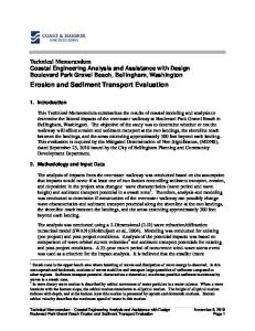
(116 inch ) layer of sediment. This allows a direct observation of the zone of the critical shear stress for the initial phase of sediment motion. This will also give a representation of the predicted maximum scour extent upstream of and laterally across the orifice for plane bed conditions. Figure 5.1 shows the fixed bed covered with the Coarse sand while a constant flow rate equal to the low head, fixed bed test is maintained. This shows the zone of the critical shear stress for this test under plane bed conditions. Table 5.1 shows the extent of this region for all sediment sizes and head levels as well as the aspect ratios ⎛ R1 ⎞ ⎜ R ⎟ of the critical shear zone. 2⎠ ⎝

37

R1 R2

Figure 5.1: Fixed Bed with Sand

Table 5.1: Critical Shear Extent, Fixed Bed Run ID H18F H24F H30F H18M H24M H30M H18C H24C H30C

R1

R2

D 0.79 0.92 1.00 0.88 0.92 1.00 0.92 1.00 1.08

D 1.04 1.08 1.13 1.04 1.08 1.13 1.08 1.17 1.25

Aspect Ratio 0.85 0.86 0.93 0.87 0.90 0.92 0.75 0.94 0.98

It can be stated that for a movable bed, as the scour depth increases the velocities in the scoured region at a given location will decrease. This will reduce the shear stresses in the area as well and may fall below the critical value. However, as the sediment is scoured, the slope of the perimeter of the scour hole will increase and may eventually slough off.

38

This may result in scour zone dimensions larger than those shown in Table 5.1. Analysis of the velocity data over a fixed bed shows that the edge of the critical shear zone does not coincide with any isovel computed from velocities measured at the orifice centerline. The velocities measured at the R1 location are significantly greater than the velocities at the R2 location. However, velocity data near the bed will be needed to verify that the edge of the zone is not an isovel. It is also noted that the aspect ratio of the critical shear zone increases with head, indicating that the shape of the scoured zone shifts from an ellipse to a circle. Another observation during this run was that there were no vortices present in the flow. Figure 5.2 shows dye placed along the bed of the model and drawn in towards the orifice.

39

Figure 5.2: Dye Visualization, Fixed Bed

The dye moved towards the orifice radially. The darkest dye trail visible is located just above the bed and clearly shows that there is no vortex present in the region upstream of the orifice under flat bed conditions.

Vortex Development

A movable bed test provided the images for this section. The bed was started from level conditions flush with the invert of the orifice. This run used the Coarse sediment and a constant head of 18 inches. The times listed below are referenced from the start of the test.

40

Initially, the sediment is drawn towards the orifice radially across the surface of the bed. It appears to draw from a region similar in shape and area to that shown in the fixed bed conditions of Figure 5.1. The sediment appears to lift from the bed and become suspended in flow before being carried out of the orifice (following the streamlines). This stage lasts for the first 30 seconds to one minute and is shown in Figure 5.3. It appears that the primary mechanism of sediment transport during this initial stage is the excess bed shear stress.

Figure 5.3: Initial Burst

After this initial motion, two counter-rotating vortices begin to form below the invert of the orifice just flanking the centerline. It should be noted that the vortices begin to form while most of the sediment is still moving radially. During this stage, the vortices at the

41

orifice help lift the sediment near the orifice into the main flow. Both scour mechanisms operate simultaneously for a very brief period of time. After this short transition period (lasting less than 10 seconds) the vortices near the orifice become the dominant mechanism for removing sediment from the scour hole. These vortices are shown in Figure 5.4, also illustrating minimal radial sediment transport in the scoured area. Looking at them from above, the one on the left rotates clockwise and the one on the right rotates counter-clockwise.

Figure 5.4: Dual Vortices

While the vortices are not the same size in this picture, they grow and shrink in alternating patterns through the entire scouring process. Sediment particles begin to roll

42

down the sides of the scoured area until they reach the vortex. They then get entrained in the vortex and sucked vertically out of the scour hole and through the orifice. There is always a vortex within the scour hole from this stage onward. However, after the scour hole grows for approximately five minutes, one vortex dominates the other to the point that the small one is not visible any more. Figure 5.5 shows one large vortex after it has eliminated the second one. Depending on which vortex has been eliminated, the single vortex may rotate in the other direction.

Figure 5.5: Single Vortex

An interesting feature to note is that the sediment is fed into the vortex in spiral shape as evident from the ridges in the figure. Some ridges are oriented parallel to the orifice face rather than pointing radially towards the outlet. Their orientation and shape

43

are driven by the vortex structure now and appear to be less dependent on the primary direction of flow. This implies that the scour processes are dependent on the vortex much more than the velocity field. As the scoured area develops further (approximately 8 minutes into the process) the second vortex returns and the vortices begin drifting around the scour hole. Figure 5.6 shows a vortex that has moved upstream from the orifice face while its counterpart remains below the invert. Figure 5.7 shows a well-defined vortex core stretching from the bed up into the flow.

Figure 5.6: Drifting Vortices

44

Figure 5.7: Vortex Core

As the scour hole develops, the vortices come and go, strengthen and weaken, sweep around the scoured area, and eventually carve out a rather large hole. The final scouring phase sees the appearance of a dominant ridge structure within the scour hole as shown in Figure 5.8.

This ridge alternately forms and is eroded throughout the

development process and becomes a permanent fixture after a time of 20-25 minutes. The vortices continue sweeping throughout the scoured area removing sediment from the base of the scour hole.

45

Center Ridge

Base Pile and Ridge Vortex

Figure 5.8: Vortex, Center Ridge, and Base Ridge

The center ridge often starts relatively straight (normal to the orifice) and begins to weave from side to side as the vortices continue to remove sediment. The sediment is always moving towards the ridge rather than in the direction of the primary flow field. The depth of the scour hole is determined by the strength of the vortices. The lateral and longitudinal extent of the scour hole is determined by the interaction of vortex induced erosion at the base of the slope and sediment trying to maintain a stable angle. This is observed by measuring the centerline scour profile during the development of the hole. These profiles show alternating pattern of base scour and sloughing of the side slopes and are shown in Fig. 5.9.

46

0.0 -0.1 -0.2 -0.3

z

D -0.4 -0.5

5hrs 20hrs

-0.6

28hrs 93hrs

-0.7 0.0

0.5

1.0

x

1.5

2.0

D

Figure 5.9: Time Variation of Centerline Bed Profile

Figure 5.10 shows the final scour hole shape after a run was completed. The perspective view shows the vertical scale of the many ridges and troughs that develop due to the drifting vortices. The centerline ridge is visible in this image, as is a well-defined ridge near the base of the scour hole. The base ridge demarcates the area of high vortex activity from the low. The vortices are located primarily in the area close to the orifice. It is clear from this figure that the equilibrium scoured area for a movable bed is much larger than the scoured area over the sediment-covered fixed bed shown in Figure 5.1.

47

Base Ridge

Center Ridge

Figure 5.10: Final Scour Hole - Perspective View

It is concluded that the size of the scoured area is dependent primarily upon the vortex structure that develops underneath the orifice and its interaction with the angle of repose of the sand. The appearance of the vortex structure is dependent upon the initial radial scour creating a depression below the orifice, but the majority of the removed sediment from the scour hole is a result of vortex-induced motion. Other runs showed similar behavior in terms of scour hole and flow field development.

48

CHAPTER 6: BED SCOUR PROFILES

As observed in the experiment and confirmed by video analysis, vortices inside the scour hole are the primary mechanism for sediment transport in this region and the growth of the scour hole.

However, the scour holes show similar patterns in the

longitudinal and transverse directions for all runs. The scour depth, length, and width for all runs as well as their corresponding critical shear zone dimensions are shown below in Table 6.1. The aspect ratios of the scour zone for the movable bed runs (AR-MB) are shown and compared to those of the critical shear zone above the fixed bed (AR-FB).

Table 6.1: Scour Hole Parameters Run ID H18F H24F H30F H18M H24M H30M H18C H24C H30C

SD

D 0.60 0.61 0.71 0.55 0.57 0.65 0.50 0.63 0.58

SL

D 1.67 1.83 2.17 1.67 1.83 2.00 1.50 1.92 2.00

R1

SW

D 1.96 2.13 2.33 1.92 2.04 2.17 2.00 2.04 2.04

D 0.79 0.92 1.00 0.88 0.42 1.00 0.92 1.00 1.08

R2

D 1.04 1.08 1.13 1.04 1.08 1.13 1.08 1.17 1.25

ARMB 0.76 0.85 0.89 0.84 0.85 0.89 0.85 0.86 0.87

ARFB 0.85 0.86 0.93 0.87 0.90 0.92 0.75 0.94 0.98

The results show that for a given sediment size, the size of the scour hole increases with head. The increase in scour hole with head is more pronounced for finer sediment. It is also noted that while the aspect ratios for movable bed scour holes generally increases with head level, they are generally smaller than the aspect ratio of their corresponding

49

fixed bed critical shear zones.

This chapter focuses on non-dimensional (ND)

comparisons of the size and shape of the scoured area based on dimensional analysis. General relationships will be determined within the experimental range of the variables.

Centerline Profiles

The centerline bed profile is taken along the x-axis upstream of the orifice. Due to instrument constraints, the bed elevation upstream of the orifice could only be measured with the ADV past a distance of x = 1.5 inches. The bed elevation flush with the wall beneath the orifice invert was checked for multiple runs and it was noted that the bed elevation at this location (x = 0) was very near to the bed elevation at x = 1.5 inches. This indicates that the bed elevations recorded with the ADV provide an accurate measure of the maximum scour depth and that the scour depth at x = 1.5 can be used to define the scour depth at x = 0. Similar observation of flat area has been recorded for scour around abutments (Dey and Barbhuiya, 2005). Figure 6.1 shows the non-dimensional centerline bed profiles for the Fine sand for various head levels and flow rates. The abscissa shows the distance upstream of the orifice and the ordinate shows the scour depth (SD), both non-dimensionalized using orifice diameter.

50

0.0

-0.5

SD

D -1.0

-1.5

H18F

CQ H19F

H24F

CQ H25F

H30F

CQ H31F

-2.0 0.0

0.5

1.0

1.5

x

2.0

2.5

D

Figure 6.1: Centerline Bed Profiles, Fine Sediment

The results show that the scour depth increases as the head and flow rate increase. The H24F centerline profile shows values higher than those of the lower heads. This is a discrepancy caused by the centerline ridge positioning itself along the centerline profile. The Medium sand and Coarse sand plots are shown in Appendix A and follow similar trends as this figure. The upper slope of the profiles for the Fine sediment in Figure 6.1 is approximately 30 degrees. The angles for the scour profiles of the Medium and Coarse sediments are both approximately 21 degrees.

51

Also of importance is the variation of the centerline profile with sediment size. Figure 6.2 shows the variation of the bed for the low head runs for different sediment size. The other heads show similar trends and are shown in Appendix A.

0.0

-0.5

SD

D -1.0

H18F

-1.5

H18M H18C -2.0 0.0

0.5

1.0

1.5

x

2.0

2.5

D

Figure 6.2: Centerline Bed Profiles, Low Head

This plot shows that the scour depth decreases with an increase in sediment size for a given head. It can be noted that the location of the upstream edge of the scour hole is nearly identical between all three cases while the scour depth shows distinct differences. This is a result of the vortex within the scour hole. If the shear stress was the primary factor defining sediment removal then the length of the scour hole would also vary with

52

sediment size. This further supports the description in Chapter 5 of the vortex as the primary mechanism of sediment removal from the scour hole. All of the centerline bed profiles appear to have the same shape when nondimensionalized (ND) with maximum scour depth along the centerline (SDCL − M ) and the scour length (SL). Figure 6.3 shows this comparison. The comparisons of centerline bed profiles for a given sediment size and varying heads are shown in Appendix A. The figure shows a transition function that has been fitted to the profile. This function and its fit parameters are shown in Appendix C. However, the shape of the profile can also be approximated by two linear relationships shown below as Equations 6.1 and 6.2.

0.0

-0.2

H18F

H24F

H30F

H18M

H24M

H30M

H18C

H24C

H30C

EQN -0.4

SD CL

SD CL − M -0.6

-0.8

-1.0 0.0

0.2

0.4

0.6

x

0.8

1.0

SL

Figure 6.3: ND Centerline Scour Profiles, All Heads and Sediments, Transition Equation

53

SDCL = SDCL − M

for x

( SL) + 1.1765

SDCL = −1.1765 x

SL

< 0.15

for 0.15 ≤ x

(6.1)

SL