Robust methods for feature extraction from mobile laser scanning 3D point clouds Abdul Nurunnabi†, Geoff West‡, David Belton‡ Department of Spatial Sciences Curtin University, Perth, Australia CRC for Spatial Information (CRCSI) †
[email protected], ‡{g.west, d.belton}@ curtin.edu.au
Abstract Three dimensional point cloud data obtained from mobile laser scanning systems commonly contain outliers. In the presence of outliers most of the currently used methods such as principal component analysis for point cloud processing and feature extraction produce inaccurate and unreliable results. This paper investigates the problems of outliers, and explores advantages of recently introduced statistically robust methods for automatic robust feature extraction. The robust algorithms outperform classical methods and show distinct advantages over well-known robust methods such as RANSAC in terms of accuracy and robustness. This paper shows the importance and advantages of several recently introduced robust statistics based algorithms for (i) planar surface fitting, (ii) surface normal estimation, (iii) edge detection, and (iv) segmentation. Experimental results for real mobile laser scanning point cloud data consisting of planar and non-planar complex objects surfaces show the proposed robust methods are more accurate and robust. The robust algorithms have potential for surface reconstruction, 3D modelling, registration, and quality control for point cloud data.
1
Introduction and Motivation
Mobile Mapping System (MMS) is an emerging technology for acquiring a three-Dimensional (3D) survey of the environment and objects in the vicinity of the mapping vehicle accurately, quickly and safely. Laser scanning provides explicit and dense 3D measurements that generate sparse point clouds. Due to its cost effectiveness and reasonable data accuracy it has been used in many applications including smart city modelling, road and rail corridor asset and inventory maintenance and management, environmental monitoring, accidental investigation, industrial control, construction management, archaeological studies, marine and coastal surveying, change detection for military and security forces, man-induced and natural disaster management (Tao and Li, 2007; Vosselman and Maas, 2010). A MMS incorporates various navigation and sensors on a common moving platform. The vehicle (Figure 1) has advanced imaging and ranging devices, such as cameras, laser scanners or Light Detection and Ranging (LiDAR) systems, and navigation/positioning/geo-referencing devices such as a Global Navigation Satellite System (GNSS) for the determination of the position of the moving platform. An Inertial Measurement Unit (IMU) that contains sensors to detect rotation and acceleration used for determining the local orientation of the platform. A Distance Measurement Instrument is often connected to a wheel of the vehicle to provide linear distance in case of GNSS outage. The continuous integration between GNSS and IMU deals with a possible loss of signal sent by the satellite and to constantly maintain the high accuracy of data acquisition. A computer with storage and operational software is used to control the data acquisition task. Laser scanners mounted on the platform (usually at a 45o angle to the vehicle track) swing the laser beam through 360o and time-of-flight is used to determine the distance to Copyright © by the paper’s authors. Copying permitted only for private and academic purposes. In: B. Veenendaal and A. Kealy (Eds.): Research@Locate'15, Brisbane, Australia, 10-12March 2015, published at http://ceur-ws.org
Research@Locate '15
109
targets. The unit can rotate up to 200 revolutions per second and the laser records points at frequencies of up to 200 kHz. Performance includes a spatial resolution of up to 1 cm at 50 km/hour, range > 100 metres (with 20% reflectivity), and measurement precision ±7 mm (Arditi et al., 2010). These configurations and advantages vary for different systems. MMSs are now able to collect more than 600,000 points per second. To extract 3D coordinates of objects and features from the geo-referenced images, modelling and data fusion are required. MMSs produce huge volumes of 3D geospatial point cloud data (Figure 2) defined by their x,y,z coordinates (or latitude, longitude and elevation). Point cloud data may have colour r,g,b information from co-registered cameras and intensity from the reflected laser beam. The output point cloud data is generally stored in an industry standard format (such as LAS), which encodes the data into a point based binary or text file.
Figure 1: Mobile mapping vehicle with onboard sensors; (curtesy: Department of Spatial Sciences, Curtin University).
Figure 2: Mobile laser scanning point cloud data with laser intensity (curtesy of AAM1). 1
http://www.aamgroup.com/
Research@Locate '15
110
Important tasks in point cloud processing include feature extraction, visualization, analysis, modelling, surface fitting, and reconstruction. Segmentation is required for surface reconstruction, feature extraction, object recognition and modelling (Pfeifer and Briese, 2007). For surface reconstruction, the quality of the results depends on the quality of estimated local surface normals. The data acquired from MMSs typically contains regions of particular surface shape (planes, cylinders), undefined surface shape, of complex topology and geometrical discontinuities, inconsistent point density, sharp features, missing points that can create holes, and features varying in size, density and complexity. Moreover, it is unreasonable to think of point cloud data without outliers. Outliers may occur because of noise, occlusions, multiple reflectance, objects getting in the way including rain, birds and other unimportant features w.r.t. the specific study (Leslar et al, 2010). Inclusion of outliers in point cloud data exacerbates the problems for reliable and robust point cloud processing and feature extraction tasks. The presence of outliers affects the estimates of normal and curvature, resulting in misleading and inconsistent results. Outliers can be dealt with by robust methods that have been widely used in computer vision, machine learning, pattern recognition, photogrammetry, remote sensing and statistics (Rousseeuw and Leroy, 2003; Meer, 2004). In spite of the recognition of outlier, many applications still use classical non-robust techniques including Least Squares (LS) and Principal Component Analysis (PCA) for point cloud processing tasks (Rabbani et al., 2006). It is well known that most of the classical techniques work well only for high-quality data and fail to perform adequately in the presence of outliers, giving inconsistent and misleading estimates of the model parameters (Nurunnabi et al., 2012a; 2014). In this paper we investigate outlier problems in classical methods as well as in robust methods such as RANSAC (Fischler and Bolles, 1981) that have been widely used for feature extraction and other point cloud processing tasks. We present some recently introduced robust methods those have been developed based on robust statistical techniques as a solution to outlier influence. This will be demonstrated through four essential point cloud processing tasks: planar surface fitting, robust local saliency features (normals and curvature) estimation, edge detection, and segmentation. The paper is organised as follows. In Section 2, the relevant literature is briefly discussed. Section 3 gives some general ideas about relevant principles and methods used in feature extraction. Robust feature extraction methods are discussed in Section 4. The limitations of the classical methods and advantages of the robust statistical methods are highlighted using real MMS acquired point cloud datasets in Section 5. Section 6 concludes the paper.
2
Background
Accurate plane fitting and the resultant estimates of the plane parameters are essential in point cloud data processing because of the presence of planar objects in the built environment. The LS method is the most wellknown classical method for model parameter estimation (Klasing et al., 2009). Hoppe et al. (1992) introduced PCA for plane fitting that has been subsequently used and extended by many authors for point cloud processing (Pauly et al., 2002; Rabbani et al., 2006; Sanchez and Zakhor, 2012). Nurunnabi et al. (2014) showed that PCA based planar surface fitting is better than LS based fitting. Fleishman et al. (2005) proposed a forward-search approach based on a robust moving least squares (Levin, 2003) technique for reconstructing a piecewise smooth surface. The method can deal with multiple outliers, but it requires very dense sampling and a robust initial estimator to initialize the algorithm. The RANSAC algorithm has been used frequently for planar surface fitting and extraction (Schnabel et al., 2007; Masuda et al., 2013). RANSAC is very efficient for detecting large planes in noisy point clouds (Deschaud and Goulette, 2010). The Hough Transform (Duda and Hart, 1972) has been used to detect geometric shapes and for plane detection in point clouds (Borrmann et al., 2011). Many methods have been developed to improve the quality of estimated normals and curvatures. Combinatorial and numerical approaches (Dey et al., 2005; Castillo et al., 2013) are two methods for normal estimation. Dey et al. (2005) developed combinatorial methods for estimating normals in the presence of noise, but in general, this approach becomes infeasible for large datasets. Hoppe et al. (1992) estimated the normal at each point to the fitted plane of nearest neighbours by applying the ‘total least squares’ method, which can be computed efficiently by PCA. PCA based plane fitting can be shown to be equivalent to the Maximum Likelihood Estimation (MLE) method (Wang et al., 2001). Distance weighting (Alexa et al., 2001), changing neighbourhood size (Mitra et al., 2004) and higher-order fitting (Rabbani et al., 2006) algorithms have been developed to modify PCA for better accuracy near sharp features and to avoid the influence of outliers on the estimates. Oztireli et al. (2009) used local kernel regression to reconstruct sharp features. However Weber et al. (2012) claimed there is a problem with the reconstruction from Oztireli et al. (2009) as it does not have a tangent plane at a discontinuous sharp feature. Segmentation groups the data points into a number of locally uniform regions. Algorithms proposed can be organised roughly into three types: edge and/or border based, region growing based, and hybrid (Koster and Spann, 2000; Huang and Menq, 2001). In edge/border based methods, points positioned on the edges/borders are detected, and then points are grouped within the identified boundaries and connected edges. In region growing algorithms, generally a seed point is chosen, and then local neighbours of the seed point are combined with the seed point if they have similar surface point properties. Many authors claim that region growing based methods suffer from over
Research@Locate '15
111
and under segmentation (Liu and Xiang, 2008). This is overcome by hybrid methods that comprise both the boundary/edge and region growing based approaches (Woo et al., 2002). Marshall et al. (2001) used LS fitting and identified surfaces of known geometric features within a segmentation framework. Klasing et al. (2009) identified the limitations of high computational cost for a large number of features. Poppinga et al. (2008) developed an efficient method of plane fitting by mean squared error computation. Castillo et al. (2013) introduced a point cloud segmentation method using surface normals computed by the constrained nonlinear least squares approach.
3
Related Classical and Robust Methods used in Feature Extraction
3.1
Principal Component Analysis and Robust Principal Component Analysis
PCA is one of the most popular multidimensional statistical techniques for dimension reduction and data visualization (Johnson and Wichern, 2002). It finds a small number d of linear combinations of the m observed variables that can represent most of the variability of the data. Data transformation generates a new set of uncorrelated and orthogonal variables that can explain the underlying covariance structure of the data. The new set of variables (the linear combinations of the mean centered original variables) called Principal Components (PCs) produce the corresponding directions using the eigenvectors of the covariance matrix (Johnson and Wichern, 2002). Many point cloud processing methods analyze the nature of the data for a local neighbourhood of a point of interest 𝑝𝑖 (𝑥𝑖 , 𝑦𝑖 , 𝑧𝑖 ) through the study of the covariance matrix of the neighbourhood. Performing Singular Value Decomposition (SVD; Searle, 2006) on the covariance matrix C of k neighbouring points of 𝑝𝑖 , 1
𝐶3×3 = 𝑘 ∑𝑘𝑖=1(𝑝𝑖 − 𝑝̅ ) (𝑝𝑖 − 𝑝̅ )𝑇 ,
(1)
where 𝑝̅ is the centre of the data, and solving the eigenvalue equation: 𝜆𝑉 = 𝐶𝑉,
(2)
produces the diagonal matrix of eigenvalues as its diagonal elements 𝜆𝑖 , and the eigenvector matrix V that contains eigenvectors or PCs as its columns. Given the required eigenvectors and the corresponding eigenvalues, C can be rewritten as: 𝐶 = ∑2𝑖=0 𝜆𝑖 𝑣𝑖 𝑣𝑖𝑇 ,
(3)
where 𝜆𝑖 and 𝜐𝑖 are the ith eigenvalue and eigenvector, respectively. The eigenvalues denote the variances along the associated eigenvectors (Johnson and Wichern, 2002). The PCs are usually ranked in descending order of explanation of the underlying data variability. Robust Principal Component Analysis (RPCA) is a robust version of PCA for determining the PCs that are resistant to outliers (Hubert et al., 2005; Feng et al., 2012). For processing 3D point cloud data, where the number of dimensions of a point is very small comparing with the number of points, an efficient method developed by Hubert et al. (2005) has been shown to give good results (Nurunnabi et al., 2014). The method maximizes certain robust estimates of univariate variance to obtain consecutive directions on which the data are projected. Hubert et al. (2005) coupled the ideas of using the robust estimator of the covariance matrix and the well-known Projection Pursuit method (PP) to use advantages from both the approaches. In the RPCA (Hubert et al., 2005), the data are pre-processed to make sure that the transformed data are lying in a subspace whose dimension is less than the number of observations. A useful way for reducing the data space is by using the SVD on the mean-centred data matrix. Then, the h points, where 𝑛/2 < ℎ < 𝑛, i.e. the “least outlying” data points are identified, and a measure of outlyingness is computed by projecting all the data points onto many univariate directions, each of which passes through two individual data points. In order to speed up the computation, the data set is compressed to PCs defining potential directions. Then, every direction for a point 𝑝𝑖 is scored by its corresponding value of outlyingness (Stahel, 1981; Donoho, 1982): 𝑤𝑖 = arg max𝑣
|𝑝𝑖 𝑣 𝑇 −𝑐MCD (𝑝𝑖 𝑣 𝑇 )| ΣMCD (𝑝𝑖𝑣 𝑇 )
,
𝑖 = 1,2, … , 𝑛
(4)
where 𝑝𝑖 𝑣 𝑇 denotes a projection of the ith observation onto the v direction, and 𝑐MCD and ΣMCD are the FMCD (Rousseeuw and van Driessen, 1999) based mean and scatter (covariance matrix) on an univariate direction v. The FMCD based estimators are used as the robust estimators of the mean and scatter in Eq. (4). In the next step, an assumed h (ℎ > 𝑛/2) portion of observations with the smallest outlyingness values are used to construct a robust covariance matrix Σℎ . A larger h can give a more accurate RPCA and a smaller h is better for more robust results. In this paper for the RPCA we use ℎ = ⌈0.5 × 𝑛⌉. Then, the method projects all the remaining observations onto the d dimensional subspace spanned by the d largest eigenvectors of Σℎ , and computes the mean and the covariance matrix by means of the reweighted MCD estimator, with weights based on the robust distance of every point. The
Research@Locate '15
112
eigenvectors of this covariance matrix from the reweighted observations are the final robust PCs. Using RPCA has the advantages of yielding accurate estimates of outlier free datasets and more robust estimates for contaminated data. In addition, it has the further advantage of classification of points into inliers and outliers (Hubert et al., 2005). Hubert et al. (2012) developed a deterministic algorithm for the MCD (DetMCD) to get the robust mean vector and covariance matrix. It uses the same iteration step but does not draw a random subset. Rather it starts from only a few well-defined initial estimators. The authors claimed that DetMCD is much faster than FMCD and is at least as robust as FMCD. The DetMCD (Hubert et al., 2012) based mean vector and covariance matrix in Eq. (4) can find outlying cases, and use of the DetMCD based mean vector and robust covariance matrix in relevant places in the RPCA algorithm produces the DetMCD based RPCA, which is called Deterministic robust PCA (DetRPCA). 3.2
RANdom SAmple and Consensus (RANSAC)
Fischler and Bolles (1981) developed a model-based robust approach: RANdom SAmple Consensus (RANSAC) that has been used in many applications for estimating model parameters from outlier contaminated data such as planar surface fitting, extraction and normal estimation in computer vision, photogrammetry and remote sensing. It can tolerate a large fraction of outliers, depending on the complexity of the model, up to and above 50%. RANSAC classifies data into inliers and outliers by using the LS cost function with maximum support (the number of data points that match with the model). It consists of two steps. First, a subset is randomly sampled and the required model parameters are estimated based on the subset. The size of the subset should be minimal of the random subset that is enough to estimate the model parameters (three points for a plane). In the second step, the model is compared with the data and its support is determined. This two-step iterative process continues until the likelihood of getting a model with better support than the current best model is lower than a given threshold, usually 1% to 5%.
4
Robust Algorithms for Feature Extraction
In this section we discuss recently introduced robust statistics based algorithms for both low level and high level feature extraction. We estimate normals and curvature as the low level saliency features that are later used for high level feature extraction. We also detect sharp features such as object edges and corners as the low level features. In this paper we perform robust segmentation (Nurunnabi et al. 2012b) to get individual surfaces (high level features) for the objects acquired by MMS. The methods for feature extraction used in this paper consist of four related tasks (Figure 3): (i) Plane fitting, (ii) edge detection, (iii) normal estimation, and (iv) segmentation.
Figure 3: Feature extraction process Using PCA for 3D point cloud data, the first two PCs form an orthogonal basis for the best-fit-plane, explaining the most variability. The third PC corresponding with the least eigenvalue expresses the least amount of variation, which defines the normal to the fitted plane. The elements of the third PC are used as the estimates of the plane parameters. The PCs (eigenvectors) 𝜈2 , 𝜈1 and 𝜈0 can be arranged according to the corresponding eigenvalues 𝜆2, 𝜆1 and 𝜆0. Thus 𝜈0 approximates the normal 𝑛̂ of the surface, and 𝜆0 indicates the surface variation along the normal. It is known that PCA is extremely sensitive to outliers, so in the following algorithms RPCA is used. Pauly et al. (2002) defined surface variation or curvature as: 𝜆0
𝜎𝑝 = ∑2
𝑖=0 𝜆𝑖
,
𝜆0 ≤ 𝜆1 ≤ 𝜆2.
(5)
Nurunnabi et al. (2012a) developed the method for edge detection in point cloud data, where the ith point is an edge point if 𝜆0 ≥ mean (𝜆0 ) + 1 × standard deviation (𝜆0 ).
Research@Locate '15
113
(6)
In this paper, we use the robust segmentation algorithm (Nurunnabi et al., 2012b) that is based on robust saliency features using DetRPCA. The robust segmentation algorithm uses a region growing approach, where the region growing starts with the least curvature value 𝜎𝑝 in Eq. (5). It uses the k nearest neighbours defined as the neighbourhood 𝑁𝑝𝑖 for every point in the data. A local planar surface is determined for every point and its neighbourhood in the point cloud using the DetRPCA algorithm. Three measures are used by DetRPCA: Orthogonal Distance OD𝑖 for the ith seed point 𝑝𝑖 to its best-fit-plane, Euclidian Distance ED𝑖𝑗 between the seed point 𝑝𝑖 and one of its neighbours 𝑝𝑗 , and angle 𝜃𝑖𝑗 between two points 𝑝𝑖 and 𝑝𝑗 . These are defined as: OD𝑖 = (𝑝𝑖 − 𝑝̅ )𝑇 . 𝑛̂,
(7)
where 𝑝̅ and 𝑛̂ are the centre and the unit normal for the fitted plane for 𝑝𝑖 , ED𝑖𝑗 = ‖𝑝𝑖 − 𝑝𝑗 ‖,
(8)
𝜃𝑖𝑗 = arccos|𝑛̂𝑖𝑇 . 𝑛̂𝑗 |,
(9)
and
where 𝑛̂𝑖 and 𝑛̂𝑗 are the unit normals for the ith seed point and one of its neighbours 𝑝𝑗 . The segmentation algorithm grows region by adding more neighbouring points one at a time from the set of data points P to the current region 𝑅𝑐 and to the seed point list 𝑆𝑐 using the following conditions: (i) OD𝑖 < OD𝑡ℎ , (ii) ED𝑖𝑗 < ED𝑡ℎ , and (iii) 𝜃𝑖𝑗 < 𝜃𝑡ℎ ,
(10)
where the OD threshold OD𝑡ℎ = median {OD (𝑁𝑝𝑖 )} + 2 × MAD {OD (𝑁𝑝𝑖 )}, {OD (𝑁𝑝𝑖 )} is the set of all OD in the 𝑁𝑝𝑖 , MAD is the Median Absolute Deviation for all the ODs in 𝑁𝑝𝑖 , and ED threshold ED𝑡ℎ = median {ED𝑖𝑗 }. If the 𝑝𝑗 fulfil the above conditions in Eq. (10) then the point is removed from the data P and considered as the next seed point for the region 𝑅𝑐 . 𝑅𝑐 grows until no new point is available in 𝑆𝑐 . After completing the region 𝑅𝑐 , the next seed point is selected from the remaining points in P in a similar fashion as the first one, and the process of region growing continues until P is empty.
5
Demonstration of the Algorithms and Results Evaluation
In this section we demonstrate the algorithms for planar surface fitting, edge detection, normal estimation, and segmentation. We explore the effects of outliers on the results based on PCA, RANSAC and DetRPCA on real MMS 3D point clouds. The results presented are mainly qualitative as it is difficult, many times, to quantitatively present results compared to, say, ground truth because of the wide variation in the results that depend on the position of outliers and the shape of the surfaces. However the results shown are representative of what would be achieved in reality. 5.1
Planar Surface Fitting
We consider the MMS dataset shown in Figure 4a. This figure shows a house and a tree with the planar surface (roof) of interest marked as blue. We label this dataset as the ‘roof’ dataset. The roof plane contains 2293 points, many of which have neighbouring points in the tree. The task is to isolate the roof from the rest of the data requiring the tree points to be detected as outliers. Figure 4b shows the points used to fit a plane using PCA (magenta), which deviate from the orientation of the original points (green) because of the influence of the outlying points in the tree. The black ellipses in Figure 4e shows the fitted and extracted plane contains many outliers projected onto the 2D approximation. That means, the outliers appear as inliers in the PCA determined plane, which clearly shows the masking effect (Hadi and Simonoff, 1993) caused by the presence of multiple outliers. We also use RANSAC algorithm for finding outliers and after removing the outlier points we fit a plane by the classical PCA, which is a diagnostic approach. The RANSAC results are in Figure 4 (c and f). Figure 4f shows many points are missing in the black rectangle and some outliers are still present in the black ellipse. Although RANSAC plane is better because the orientation of the fitted plane (magenta) in Figure 4c is almost coincides to the real points but the fitted plane (magenta) for PCA in Figure 4b is significantly distracted by the outliers. Now we perform DetMCD based RPCA (DetRPCA) to fit the plane. Results in Figure 4d shows that the fitted plane is in right direction without the effect of outliers, and the resultant extracted final plane in Figure 4g is clearly free from the effect of outlier without showing any masking effect. That means, DetRPCA results are robust to outliers.
Research@Locate '15
114
Figure 4: Plane fitting and identification for (a) roof and tree dataset surrounded by a tree, the roof points are in blue. Plane (magenta) orientation by (b) PCA, (c) RANSAC, and (d) DetRPCA.The fitted/extracted plane by (e) PCA, (f) RANSAC, and (g) DetRPCA.
5.2
Edge Detection and Normal Estimation
We take a dataset containing part of a building (Figure 5a) consisting of 58,371 points. We label the data as the ‘building and wall’ dataset that has sharp edges and corners. To extract these sharp features we use the classification algorithm (Nurunnabi et al., 2012a). We fit a plane to each point in the data with a local neighbourhood of k = 50. We choose the value of k based on similar real data empirically. We calculate the 𝜆0 values and classify the points into inliers (surface points) and outliers (edge or corner points) according to Eq. (6). The classification results are in Figure 5(b, c and d). The results in Figure 5b show that PCA fails to recover the sharp features (edge/corner points), marked by the black ellipse and polygon. Although RANSAC (Figure 5c) is a robust method, it does not correctly classify surface, edges and corners, with many surface points appearing as edge points. Figure 5d shows that the proposed DetRPCA is significantly more accurate than PCA and RANSAC. Normals on or near sharp features become overly smooth mainly for two reasons: (i) neighbourhood points may be present locally from two or more surfaces, and (ii) the presence of outliers/noise in the local neighbourhood (Nurunnabi et al., 2014). We consider a small part from Figure 5a shown in Figure 6a where three edges and one corner are present. In Figure 6b, the PCA method counts all the points for plane fitting in a local neighbourhood and so misrepresenting the normal at the vertex and smoothing out the sharp features. Figure 6c shows that RANSAC normals are not properly estimated and oriented, with many misclassified points around the edges and corners. This is because RANSAC was unable to get the most homogeneous points within the neighbourhoods. The robust statistical method used in the DetRPCA algorithm groups the majority of points that are homogeneous w.r.t. the neighbouring points. Hence, the estimated normal represents the surface consisting of the majority of homogeneous points. In Figure 6d, we see that robust normals are correctly oriented on the corner and on the edge points and results in normals that preserve the sharp transitions while PCA and RANSAC have smoothly changing normals areas by the black lines.
Research@Locate '15
115
Figure 5: (a) The building and wall data, edge and corner point recovery (in magenta): (b) PCA, (c) RANSAC, and (d) DetRPCA.
Figure 6: (a) Point cloud data, and normal orientation for: (b) PCA, (c) RANSAC, and (d) DetRPCA. 5.3
Segmentation
For segmentation, we consider a MMS dataset shown in Figure 7a of a petrol station, consisting of many planar and non-planar surfaces described by 111,070 points. We name this the ‘petrol station’ dataset. We set the required parameters: k = 30 and angle threshold 𝜃𝑡ℎ= 7o. Segmentation results are in Figure 7 (b, c and d) in which points that belong to each region are shown in different colours. Perfect Segmentation (PS) is identified as a true segment from manually determined ground truth i.e. one segment describes a single feature such as the wall of a house that is one planar surface. Over Segmentation (OS) occurs where one true segment is broken into two or more separate segments, and Under Segmentation (US) is where more than one true segment are wrongly grouped together as one segment (Nurunnabi et al., 2014). Figure 7b
Research@Locate '15
116
shows that PCA produces the worst results and failed to segment most of the different surfaces correctly. Much OS and US occurs in different places, these are highlighted by the black ellipses. Although the results in Figure 7c look slightly better than those in Figure 7b, likewise PCA, RANSAC fails to separate the road, kerb and footpath. In Figure 7c the black ellipse on the roof shows much unwanted OS occurring. DetRPCA based segmentation results in Figure 7d show that most of the surfaces are properly segmented with very little OS and without any US, out of 76 Total Segments (TS), 62 are PS. The road, kerb and footpath are extracted correctly. Performance for the methods is evaluated quantitatively in Table 1.
Figure 7: (a) Petrol station dataset, and segmentation results for: (b) PCA, (c) RANSAC, and (d) DetRPCA. Table 1: Segmentation performance evaluation. Methods PCA RANSAC DetRPCA
6
TS 88 97 76
PS 27 32 62
OS 34 37 09
US 03 01 00
Conclusions
This paper describes some of the recently proposed algorithms for robust feature extraction in MMS 3D point cloud data. It demonstrates that robust statistics based algorithms outperform classical methods and significantly produce much better results than the popular RANSAC method. Results show the planar surfaces were fitted more robustly than the existing methods, edge and corner points were identified more accurately without any misclassification error, normals from the robust method are perfectly oriented, and segmentation results were more accurate with much less over and under segmentation. The algorithms have the limitation that the quality of the results reduces in the presence of more than 50% outliers. However, this is an extreme case but the presented algorithms are much better at dealing with this than others. The robust feature extraction methods are much better than others, and they have potential for surface reconstruction, registration and quality control for the point cloud data.
Research@Locate '15
117
Acknowledgements This study has been carried out as a PhD research supported by a Curtin University International Postgraduate Research Scholarship (IPRS). The work has been supported by the Cooperative Research Centre for Spatial Information (CRCSI), whose activities are funded by the Australian Commonwealth's Cooperative Research Centres Programme. We are also thankful to the AAM Group and McMullen Nolan and Partner Surveyors for the real point cloud datasets.
References Alexa, M., Behr, J., Cohen-Or, D., Fleishman, S., Levin, D., and Silva, C. T. (2001). Point set surfaces. In Proceedings of the 12th IEEE International Conference on Visualization, San Diego, California, USA, 21 ̶ 28. Arditi, R., Garozzo, M., Laddomada, F., Paris, R., Rossi, S., Rotondi, A., and Zampa, F. (2010). New mobile LiDAR and satellite technologies for a better knowledge of roads ̶ application to modern motorways and the case of the ancient appian way. In ASECAP Annual Study and Information Days, Oslo, Norway, 120 ̶ 128. Borrmann, D., Elseberg, J., Lingemann, K., and N• uchter, A. (2011). The 3D Hough Transform for plane detection in point clouds: a review and a new accumulator design. 3D Research, Springer 2(2), 1 ̶ 13. Castillo, E., Liang, J., and Zhao, H. (2013). Point cloud segmentation and denoising via constrained nonlinear least squares surface normal estimates. In M. Breuß, A. Bruckstein, and P. Maragos (Eds.), Innovations for Shape Analysis: Models and Algorithms, Springer, New York, USA, 283 ̶ 298. Deschaud, J.-E. and Goulette, F. (2010). A fast and accurate plane detection algorithm for large noisy point clouds using filtered normals and voxel growing. In Proceedings of the 5th International Symposium 3D Data Processing, Visualization and Transmission, Paris, France. Dey, T. K., Gang, L., and Sun, J. (2005). Normal estimation for point cloud: a comparison study for a Voronoi based method. In Proceedings of the Eurographics Symposium on Point-Based Graphics, New York, USA, 39 ̶ 46. Donoho, L. (1982). Breakdown properties of multivariate location estimators. PhD Qualifying paper, Harvard University, Boston, USA. Duda, R. O. and Hart, P. E. (1972). Use of Hough transformation to detect lines and curves in pictures. Communications of the ACM 15(1), 11 ̶ 15. Feng, J., Xu, H., and Yan, S. (2012). Robust PCA in high-dimension: a deterministic approach. In Proceedings of the 29th International Conference on Machine Learning, Edinburgh, Scotland, UK, 249 ̶ 256. Fleishman, S., Cohen-Or, D., and Silva, C. (2005). Robust moving least-squares fitting with sharp features. ACM Transactions on Graphics 24(3), 544 ̶ 552. Fischler, M. A. and Bolles, R. C. (1981). Random Sample Consensus: a paradigm for model fitting with applications to image analysis and automated cartography. Communications of the ACM 24(6), 381 ̶ 395. Hadi, A. S. and Simonoff, J. S. (1993). Procedures for the identification of outliers. Journal of the American Statistical Association 88(424), 1264 ̶ 1272. Hoppe, H., Rose, T. D., and Duchamp, T. (1992). Surface reconstruction from unorganized points. In Proceedings of the ACM SIGGRAPH (26), Chicago, USA, 71 ̶ 78. Huang, J. and Menq, C.-H. (2001). Automatic data segmentation for geometric feature extraction from unorganized 3-D coordinate points. IEEE Transactions on Robotics and Automation 17(3), 268 ̶ 279. Hubert, M., Rousseeuw, P. J., and Branden, K. V. (2005). ROBPCA: a new approach to robust principal component analysis. Technometrics 47(1), 64 ̶ 79. Hubert, M., Rousseeuw, P. J., and Verdonck, T. (2012). A deterministic algorithm for robust scatter and location. Journal of Computational and Graphical Statistics 21(3), 618 ̶ 637. Johnson, R. A. and Wichern, D. W. (2002). Applied Multivariate Statistical Analysis. Prentice Hall, New Jersey, USA, 5th edition.
Research@Locate '15
118
Klasing, L., Altho_, D., Wollherr, D., and Buss, M. (2009). Comparison of surface normal estimation methods for range sensing applications. In Proceedings of the IEEE International Conference on Robotics and Automation, Kobe, Japan, 3206 ̶ 3211. Koster, K. and Spann, M. (2000). MIR: an approach to robust clustering-application to range image segmentation. IEEE Transactions on Pattern Analysis and Machine Intelligence 22(5), 430 ̶ 444. Leslar, M., Wang, J. G., and Hu, B. (2010). A comparison of two new methods of outlier detection for mobile terrestrial LiDAR data. The International Archives of Photogrammetry, Remote Sensing and Spatial Information Sciences 38(Part 1), 78 ̶ 84. Levin, D. (2003). Mesh-independent surface interpolation. In Brunnett, Hamann, and Mueller (Eds.), Geometric Modeling for Scientific Visualization, Springer, New York, USA, 37 ̶ 49. Liu, Y. and Xiang, Y. (2008). Automatic segmentation of unorganized noisy point clouds based on the Gaussian map. Computer-Aided Design 40(5), 576 ̶ 594. Marshall, D., Lukacs, G., and Martin, R. (2001). Robust segmentation of primitives from range data in presence of geometric degeneracy. IEEE Transactions on Pattern Analysis and Machine Intelligence 23(3), 304 ̶ 314. Masuda, H., Tanaka, I., and Enomoto, M. (2013). Reliable surface extraction from point-clouds using scannerdependent parameters. Computer Aided Design and Applications 10(2), 265 ̶ 277. Meer, P. (2004). Robust techniques for computer vision. In G. Medioni, and S. B. Kang (Eds.), Emerging Topics in Computer Vision, Prentice Hall, New Jersey, USA,107 ̶ 190. Nurunnabi, A., Belton, D., and West, G. (2012a). Robust segmentation for multiple planar surface extraction in laser scanning 3D point cloud data. In Proceedings of the 21st International Conference on Pattern Recognition (ICPR), Tsukuba Science City, Japan, 1367 ̶ 1370. Nurunnabi, A., Belton, D., and West, G. (2012b). Robust segmentation in laser scanning 3D point cloud data. In Proceedings of the Digital Image Computing: Techniques and Applications (DICTA), Fremantle, Australia, 1 ̶ 8. Nurunnabi, A., Belton, D., and West, G. (2014). Robust statistical approaches for local planar surface fitting in 3D laser scanning data. ISPRS Journal of Photogrammetry and Remote Sensing 96, 106 ̶ 122. Öztireli, A. C., Guennebaud, G., and Gross, M. (2009). Feature preserving point set surfaces based on nonlinear kernel regression. Computer Graphics Forum 28(2), 493 ̶ 501. Pauly, M., Gross, M., and Kobbelt, L. P. (2002). Efficient simplification of point sample surface. In Proceedings of the International Conference on Visualization, Washington, D.C., USA, 163 ̶ 170. Pfeifer, N. and Briese, C. (2007). Geometrical aspects of airborne laser scanning and terrestrial laser scanning. International Archives of Photogrammetry, Remote Sensing and Spatial Information Sciences 36(Part 3/W52), 311 ̶ 319. Poppinga, J., Vaskevicius, N., Birk, A., and Pathak, K. (2008). Fast plane detection and polygonalization in noisy 3D range image. In Proceedings of the IEEE International Conference on Intelligent Robots and Systems (IROS), Nice, France, 3378 ̶ 3383. Rabbani, T., van den Heuvel, F. A., and Vosselman, G. (2006). Segmentation of point clouds using smoothness constraint. The International Archives of the Photogrammetry, Remote Sensing and Spatial Information Sciences 36(5), 248 ̶ 253. Rousseeuw, P. J. and Leroy, A. (2003). Robust Regression and Outlier Detection. John Wiley and Sons, New York, USA. Rousseeuw, P. J. and Driessen, K. V. (1999). A fast algorithm for the minimum covariance determinant estimator. Technometrics, 41(3):212 ̶ 223. Searle, S. R. (2006). Matrix Algebra Useful for Statistics. John Wiley and Sons, New York, USA. Stahel, W. A. (1981). Robust Estimation: Infinitesimal Optimality and Covariance Matrix Estimators, PhD thesis, Department of Mathematics, Eidgenossische Technische Hochschule (ETH), Zurich, Switzerland.
Research@Locate '15
119
Sanchez, V. and Zakhor, A. (2012). Planar 3D modelling of building interiors from point cloud data. In Proceedings of the IEEE International Conference on Image Processing (ICIP), Florida, USA, 1777 ̶ 1780. Schnabel, R., Wahl, R., and Klein, R. (2007). Efficient RANSAC for point-cloud shape detection. Computer Graphics Forum 26(2), 214 ̶ 226. Tao, C. V. and Li, J., Eds. (2007). Advances in Mobile Mapping Technology. Taylor and Francis Group, London, UK. Vosselman, G. and Maas, H.-G., Eds. (2010). Airborne and Terrestrial Laser Scanning. Whittles Publishing and CRC Press, Scotland, UK. Wang, C., Tanahashi, H., and Hirayu, H. (2001). Comparison of local plane fitting methods for range data. In Proceedings of the IEEE International Conference on Computer Vision and Pattern Recognition, Kauai, HI, USA, 663 ̶ 669. Weber, C., Hahmann, S., Hagen, H., and Bonneau, G.-P. (2012). Sharp feature preserving MLS surface reconstruction based on local feature line approximations. Graphical Models 74(6), 335 ̶ 345. Woo, H., Kang, E., Wang, S. Y., and Lee, K. H. (2002). A new segmentation method for point cloud data. International Journal of Machine Tools and Manufacture 42(2), 167 ̶ 178.
Research@Locate '15
120