RNN-based Learning of Compact Maps for Efficient Robot Localization Alexander F¨ orster1 and Alex Graves1 and J¨ urgen Schmidhuber1,2
∗
1- Istituto Dalle Molle di Studi sull’Intelligenza Artificiale (IDSIA) Galleria 2, 6928 Manno-Lugano - Switzerland 2- TU M¨ unchen - Cognitive Robotics Boltzmannstr. 3, 85748 M¨ unchen-Garching - Germany Abstract. We describe a new algorithm for robot localization, efficient both in terms of memory and processing time. It transforms a stream of laser range sensor data into a probabilistic calculation of the robot’s position, using a bidirectional Long Short-Term Memory (LSTM) recurrent neural network (RNN) to learn the structure of the environment and to answer queries such as: in which room is the robot? To achieve this, the RNN builds an implicit map of the environment.
1
Introduction
Traditional approaches to Simultaneous Localization and Mapping (SLAM) with distance sensor data are typically based on occupancy grids — that is, the robot builds an explicit map of its environment as it moves around [1, 2, 3, 4]. These algorithms have to cope with uncertainty in sensor and odometry data and need to store huge amounts of data for later refinement and correction, making them expensive in memory and computation time. To reduce the amount of data in high resolution grid-based mapping some researchers convert the map into a topological map [5, 6]. However, these approaches need to build first the explicit map before transforming it, which is very resource-consuming. Our approach uses a neural network to localize the robot, trained with sequences of input data from distance sensors. Unlike other localization and mapping algorithms, our method does not generate an explicit map of the environment and does not calculate Euclidean coordinates. Instead, the RNN stores an implicit map, which matches robot positions with topological labels. Topological labels or positions, like “in the kitchen” or “next to the copy machine” represent a more natural description of the environment, which is also very memory-efficient. Unlike other neural network based localization methods we do not use artificial landmarks [7, 8] or operate in a limited environment [9]. In addition, the absence of a fixed map makes it easier to cope with problems such as moving obstacles, which hide parts of the environment, or the temporal absence of marks, like room doors hidden by obstacles. In order to maximize the temporal context available for localization, a bidirectional Long-Short Term Memory architecture is used [10, 11] for the neural ∗ This work was supported by the Sixth Framework Program of the European Union (project number IST-511931) and by the Swiss National Science Foundation (SNF grant number 2000020-100249).
network. The learning approach is robust against sensor data noise and the “kidnapping” problem: Taking the robot from its current position and placing it somewhere else without giving it any information about the replacement. The paper continues with section 2 with a description of the neural network. Section 3 describes our simulation environment and experiments, while section 4 presents and discusses the results and finally, section 5 concludes the paper.
2
Learning Method
We use a neural network to learn the mapping between sensor input data and robot locations. We use 2D laser range distance sensors, the most frequently used sensors for localization since they have an adequate resolution and a low data rate per time-step. We use the distance information directly as input data for the neural network. The outputs of the network are interpreted as the probabilities of the robot being in specific labelled areas in the environment — in other words they are used to classify the robot’s positions. In order to extend the time dependency range of contextual information when making these classifications, we use the Long Short-Term Memory (LSTM) recurrent network architecture [10]. LSTM is able to bridge longer time lags than conventional RNNs due to its use of special memory cells, whose activation is protected by multiplicative gates [12]. Many sequence classification tasks have been shown to benefit from bidirectional context, i.e. information about the future as well as the past of a particular point in the input sequence. Bidirectional recurrent neural networks (BRNNs) are an elegant method utilizing such context into RNNs [13]. BRNNs have yielded significantly improved results in several sequence classification tasks, such as protein structure prediction. In this paper we combine both techniques and use bidirectional LSTM. This combination of network structures has previously been successfully applied to speech recognition tasks [11]. The network input consists only of the information from the laser range scanner; no odometry information, orientation information or motor commands are included. The input data is normalized to have mean 0 and standard deviation 1. See Figure 1(b) for an illustration of the range measurements. The network has an input layer size of 36 (one input for each direction of the laser scanner) and an output layer size of 16 (one output for each room or area in the environment). It has two hidden layers, one for the forward and one for the backward subnet of the bidirectional architecture, each of them containing 50 LSTM blocks. All cells in the blocks have logistic sigmoid activation functions. Standard gradient descent with momentum is used for the supervised training.
3
Experiments
We used an in-house 3D simulation system to simulate the motion of a robot in a house environment. It contains 15 rooms or room-like areas, and its total size
Robot 0
10 4
5
1
7
13
11 8 12
2 3
(a)
6
9
14
(b)
Fig. 1: (a) The used simulated house environment, with the robot (black circle), obstacles (dots) and rooms labels (numbers). (b) Illustration of the robot laser range measurements for its position in (a). The lengths of the radial lines represent the measured distance to the nearest opaque object. The input is shown without (top) and with noise and obstacles (bottom). is 10.5 m by 18.9 m. The rooms have various shapes and numbers of doors, and some of them are reachable only from one other room (see Figure 1(a)). There are many cycles in the environment, which is in general one of the hardest problems to handle for traditional SLAM algorithms, especially when no odometry information is available. The simulated robot, whose design was derived from the Robertino1 platform, has a circular base with a diameter of 40 cm. The robot was equipped with a holonomic drive, a laser range scanner with an angular resolution of 10 degrees and a maximum range of 5m. Clearly, placing obstacles in such an environment will substantially influence the robot’s laser range measurements. In order to test the robustness of our system to such influences, we carried out experiments with up to 20 obstacles (slowly moving cones with a diameter of approximately 40 cm) in various locations around the house. Figure 1(a) shows a top-down view of a typical scene with 20 obstacles and Figure 1(b) shows the sensor measurements of the robot in this scene with and without noise (see below) and obstacles. We conducted 6 experiments in various scenarios by manually steering the robot in the house. Each sequence was between 69 and 1 793 time-steps long and contained visits to 2 to 37 rooms. For the first four experiments we varied the noise in the sensor data readings, but did not include any obstacles. The last two experiments had a fixed noise ratio and contained various number of obstacles. For these experiments, the training set contained sequences both with and without obstacles, while the test set contained only sequences with a fixed number of obstacles (10 for experiment five and 20 for experiment six). For each sequence, the robot and the obstacles (if present) were given random initial positions. Details about the number of recorded sequences are given in Table 1. In order to expand the size of the training set, and thus improve general1 www.openrobertino.de
Nr 1 2 3 4 5 6
Sequences Train Test 120 19 120 19 120 19 120 19 270 20 320 20
Time steps
Noise
Obstacles
34 867 34 867 34 867 34 867 70 002 106 333
0.0 0.2 0.5 1.0 0.2 0.2
0 0 0 0 10 20
Quality Train Test 95.2 % 81.8 % 92.8 % 80.1 % 91.7 % 82.7 % 92.5 % 80.1 % 93.2 % 82.8 % 73.1 % 55.4 %
Table 1: For each experiment the number of sequences and time steps for training and testing the network are given. The noise column gives the standard deviation of the simulated laser range sensor noise. The two rightmost columns show the percentage of correct classifications for the training set and the test set respectively. Target 1
0 #4
#1
#4
Output
#2
#4
#6
#2
#4
#6
1
0 #12
#4 #9
#1
#4
Fig. 2: An episode from the test set with 20 obstacles. The target values (top) and the output of the network (bottom) are shown. The labels indicate the classified room number. ization, we rotated the robot’s sensor data 35 times (from 10 to 350 degrees) and appended the rotated data to the original training set. Since the robot’s input was radially symmetrical, these rotations only had the effect of altering the robot’s initial direction, and did not change its perception of the environment. The learning rate was fixed to 10−5 with momentum 0.9 for all experiments. The training time lay between 14 and 54 epochs. Gaussian noise with standard deviation 1 was added to the data in each time-step to prevent over-fitting.
4
Results and Discussion
The two rightmost columns in Table 1 show the performance of the learning process in relation to noise and number of obstacles. The accuracy of the algorithm is not greatly influenced by noisy sensor data. The proportion of falsely classified rooms is around 20% for all noise levels with a standard deviation between 0 and 1 of the normalized data. The algorithm also appears to be robust to small numbers of obstacles. To explore the essence of the algorithm in detail, we show additionally one of the robot trails in Figure 2. A trained robot moves from room 4 to 1, back to
Target 1
0 0
50
100
150
180
250
318
250
318
250
318
Output with Reset 1
0 0
50
100
150
180
Output without Reset 1
0 0
50
100
150
180
Fig. 3: In this episode, the robot was kidnapped at time-step 180 and set instantaniously from room 6 to room 12 (top graph). The algorithm can handle the sudden event quite well (lower graph). Resetting the network at kidnapping time improves the classification (middle graph). 4, has a look into room 2, and finishes in room 6. The uncertainty in the beginning of the sequence occurs while the robot stands still in the first time-steps. The correct room is detected immediately after the robot starts moving. Neural networks are in general capable of sequence prediction as well as sequence classification, so it should be possible for the network to learn which label transitions are possible in the given environment. However, in the example in Figure 2 the network predicts (albeit with low probability) impossible transitions from room 4 to room 9 and then to room 1 in the first part of the trail. Various experiments have shown that the algorithm is also robust against the “kidnapping problem” (Figure 3). The robot was kidnapped at time-step 180 replaced from room 6 to room 12. The algorithm can handle the sudden event quite well. After a short time the robot was able to correctly localize itself. Reset of the network at the time of kidnapping clearly favors the classification, but is not needed, as seen in the lowest graph of Figure 3.
5
Conclusion and Future Work
We presented a new robot localization method very different from previously described techniques. Instead of using traditional memory-wasteful occupancy grids or building an explicit Euclidean map, we use a tiny neural network to learn a simple, implicit memory-efficient topological map. Topological maps have several advantages compared to Euclidean maps, e.g. easier path planning, memory efficiency, and a natural interpretation of the environment. Furthermore, our approach is based on distance sensor readings and does not rely on artificial landmarks, odometry or other additional sensor data.
We implemented our approach and carried out experiments on a simulated environment, with complexity not less than that of real-world applications. We achieved results of over 80% accuracy, demonstrating both the feasibility and easy applicability of the algorithm. In the future we plan to extend our method to different robot tasks, such as path planning and navigation. With some additional research, we feel that the RNN approach will be competitive with state-of-the-art localization algorithms. Additionally, we plan to apply the localization method to real laser range sensors data in real habitat environments. This will allow comparison to other well known SLAM methods.
References [1] John J. Leonard and Hugh F. Durrant-Whyte. Simultaneous map building and localization for an autonomous mobile robot. In IEEE Int. Workshop on Intelligent Robots and Systems, pages 1442–1447, Osaka, Japan, November 1991. [2] Sebastian Thrun. Robotic mapping: a survey. In Gerhard Lakemeyer and Bernhard Nebel, editors, Exploring artificial intelligence in the new millennium, pages 1–35. Morgan Kaufmann Publishers Inc., San Francisco, CA, USA, 2003. [3] Wolfram Burgard, Dieter Fox, Daniel Hennig, and Timo Schmidt. Estimating the absolute position of a mobile robot using position probability grids. In Proc. of the 14th National Conf. on Artificial Intelligence, volume 2, pages 896–901, Portland, OR, August 1996. [4] Udo Frese. A discussion of simultaneous localization and mapping. Autonomous Robots, 20(1):25–42, 2006. [5] Jens-Steffen Gutmann and Bernhard Nebel. Navigation mobiler roboter mit laserscans. In Autonome Mobile Systeme 1997, 13. Fachgespr¨ ach, pages 36–47, London, UK, 1997. Springer-Verlag. [6] Howie Choset and Keiji Nagatani. Topological simultaneous localization and mapping (slam): Toward exact localization without explicit localization. IEEE Tr. on Robotics and Automation, 17(2):125–137, April 2001. [7] Juliana F. Camapum, Mark H. Fisher, and John Potter. Possible back-propagation neural network structures for agv localization. In In Proc. 5th Int. Conf. on Optimization of Electric and Electronic Equipment, 1996. [8] Hongjun Zhou and Shigeyuki Sakane. Sensor planning for mobile robot localization – use of learning bayesian network structure –. In Conf. of the Robotics Society of Japan 2002, Osaka, October 2002. [9] Janusz Racz and Artur Dubrawski. Artificial neural network for mobile robot topological localization. J. on Robotics and Autonomous Systems, 16(1):73–80, November 1995. [10] Sepp Hochreiter, Yoshua Bengio, Paolo Frasconi, and J¨ urgen Schmidhuber. Gradient flow in recurrent nets: the difficulty of learning long-term dependcies. In John F. Kolen and Stefan C. Kremer, editors, A Field Guide to Dynamical Recurrent Neural Networks, pages 237–244. Wiley-IEEE Press, 2001. [11] Alex Graves and J¨ urgen Schmidhuber. Framewise phoneme classification with bidirectional lstm networks. In Proc. of the 2005 Int. Joint Conf. on Neural Networks, Montreal, Canada, August 2005. [12] Felix A. Gers, Nicol N. Schraudolph, and J¨rgen Schmidhuber. Learning precise timing with lstm recurrent networks. J. Mach. Learn. Res., 3:115–143, 2003. [13] Mike Schuster and Kuldip K. Paliwal. Bidirectional recurrent neural networks. IEEE Tr. on Signal Processing, 45:2673–2681, November 1997.