Risk: measures and tools
1
Contents
1. An overview of risk management evolution 2. The old risk management tools - Mean-Variance portfolio theory - CAPM and APT 3. Hedging and financial products 4. Risk measures - Coherent and convex risk measures - VaR and Expected Shortfall (CVaR, tail loss) 5. Hedging on the greeks 6. Bank regulation 7. The future of regulations: Proposals and questions 2
1 – Overview
3
1. Overview
Until the 1970’s corporate risk management was mostly buying insurance. Risk management in the financial sector was rudimentary. The market for futures and options was small and with large bidask spreads. Reasons: - Economic prejudice (Indifference theory?, CAPM) - Lack of good tools to quantify risk - Lack of distributed computing power 4
1. Overview
The risk management revolution of the 1970’s - The option pricing model of BlackScholes and Merton (1973) - Texas-Instr. hand-held calculator for BS, the personal computer (1975), VisiCalc spreadsheet (1979), Sun and Digital workstations, the Bloomberg terminal (80’s) - Chicago Board Options Exchange 5
1. Overview
Derivative markets (options, futures and swaps) began with equities, currencies and interest rates. Expanded to metals, energy and other commodities And later to credit risk Derivative values raised from $72.1012 in 1998 to $370.1012 in 2006 to $600.1012 in 2007 Meanwhile the market became very complex, up to “synthetic CDO’s” – derivatives of derivatives of derivatives 6
1. Overview
Options became of interest not only to banks, hedge and pension funds but also to other corporations as a way to grow. Corporate risks: market, financial, operational Raising capital to cover all risks makes no sense. Capital is not used efficiently. There is an ideal debt-to-equity ratio If risks can be traded, it make sense to lay-off risks for which there is no competitive advantage Therefore more equity capital may be reserved for risks that cost more to transfer than to manage. Transferring risk, more equity capital, now not needed as insurance, was available to generate new business, hence promoting growth 7
1. The mortgage market
8
1. The mortgage market and risk transfer
The current subprime crisis: Traditionally banks held their mortgages in a single portfolio The 1980’s big change: Transfer of credit risk Pooling of mortgages, dividing the pools into tranches, sold to third parties Therefore the risk of mortgage default is written out of the books of the original bank, which has capital available to make further mortgage loans (and collect the fees), mortgages which are also pooled, etc., etc 9
1. Overview
Many institutions, pension funds, hedge funds and nonmortgage banks held huge portfolios of “highly-rated” mortgage-backed securities or even CDO’s of mortgage-backed securities. In the mortgage business banks collected fees, intermediate agents collected fees, rating agencies collected fees. Conclusion: Explosive profitability of the banking sector However: the underwriting and rating of mortgages became far too “relaxed”. Agents, banks and rating agencies did not care much about the income statements of the borrowers. They just received their fees, the risk was going to be transferred anyway. Also the house prices were increasing steadily. As the subprime default rates increased, the prices of the mortgage securities dropped. 10
1. Overview
The involved banks and other institutions had to write off billions in asset values, seek large capital infusions and banks drastically reduced lending Reduced lending by banks affects all corporations, even those not involved in the mortgage-backed market, because of the equity-to-debt ratio and operations financing. Hedge funds, losing money in the subprime market, started selling positions in other markets. Stocks dropped. As the houses that were defaulted were auctioned at low prices, prices dropped even more leading to more defaults because of impossibility to refinance or the simple consideration: Why should I pay to the bank more than the house is worth? 11
12
1. Overview
Conclusions: - Without intervention, or even with it, the global economy seems heading for recession. - The “invisible hand” seems to be asleep. Maybe there never was an invisible hand in the market. - Most important: The quality of the derivatives market depends on the quality of the underlying assets. Transferring risk does not eliminate risk And in the future, what to do ? 13
1. Rescue ?
14
1. Regulation ?
15
1. Remarks
There is some trend in the financial culture to the effect that to prevent future crisis more sophisticated (mathematical) models are needed for the dynamics of the markets, as well as for the economy in general and the human behavior. That is probable true and evidence comes from the complexity of economic events, the complex nature of market fluctuations, even outside crisis, and the deviations of human behavior from simple rational models. A good opportunity for mathematicians and physicists, provided they make some effort to learn the facts. However the current crisis is not sophisticated at all. It stems from the old-fashioned facts that it is unwise to lend money to someone that cannot pay it back and also that it is easy to take risks that in end become other 16 people’s responsibility.
Nevertheless, because one always has to find someone else to blame, in the mass media, mathematicians and theoretical economists are being elected as the culprits
17
18
Model of a perfect economic system
19
2 – The old risk management tools
20
2 . The old risk management tools
There should be a trade off between risk and expected return The higher the risk, the higher the expected return, otherwise why take the risk?
21
2. Mean-variance portfolio theory Suppose bonds yield 5% and the returns for an equity investment are: Probability 0.05 0.25 0.40 0.25 0.05
Return +50% +30% +10% –10% –30% 22
2. Mean-variance portfolio theory
We can characterize investments by their expected return and standard deviation of the return For the equity investment: { {
Expected return μ = Σi pi ri = 10% Standard deviation of return σ = (Σi pi ri 2)1/2 = 18.97
The return is higher than the bond return but also the standard deviation
23
2. Combining Risky Investments σ P = w12σ 12 + w22σ 22 + 2 ρw1w2
rP = w1r1 + w2 r2 16
Ex p e cte d R e tu rn (%)
14
r1 = 10%
12
r2 = 15%
10
σ 1 = 16% σ 2 = 24% ρ12 = r1r2 = 0.2
MVP
8 6 4 S ta n d a rd De via tio n o f Re tu rn (%)
2 0 0
5
10
15
20
25
30
24
2. Combining Risky Investments -
-
Systematic risk = risk associated to the correlation Unsystematic (specific) risk associated to individual variances As the portfolio gets larger, specific risk tend to zero whereas systematic risk tends to the average of the covariances of all pairs. Only points above the minimum-variance point (MVP) are useful Points above the MVP are the efficient set (frontier) Minimizing the variance for a given return with n assets is called the Markowitz problem Given two portfolios in the efficient frontier, they generate by convex combinations all the points in the efficient frontier (The two-fund theorem) 25
2. Adding a riskless asset J
Expected Return
M
E(RM) I
Previous Efficient Frontier
F RF New Efficient Frontier
S.D. of Return
σM
26
2. Adding a riskless asset -
-
-
If borrowing the riskless asset (at the same interest rate) is allowed, the new efficient frontier is the line FIMJ If borrowing is not allowed it is the line FIM plus the rounded part of the previous efficient frontier The portfolio M and the riskless asset generate all of the efficient frontier (The one-fund theorem) 27
2. The Capital Asset Pricing Model (CAPM) -
-
-
-
Assumptions: # All investors are mean-variance optimizers with the same expectations # No transaction costs By the one-fund theorem, all investors will hold a mixture of the riskless asset and the portfolio M. Because all risky assets must be held by someone, M must contain all risky assets. It is called the market portfolio The efficient frontier is the capital market line
28
2. The Capital Asset Pricing Model (CAPM) Expected Return E(R)
E(RM)
M
E (RM ) − RF
σM
= Sharpe ratio
E ( R ) − RF = β [ E ( RM ) − RF ]
RF
Beta
1.0
σ β= σM 29
2. Arbitrage Pricing Theory
Instead of having to estimate n expected returns and n(n+1)/2 covariances consider the returns to depend on a smaller number of factors We can form portfolios to eliminate the dependence on the factors Leads to the result that expected return is linearly dependent on the realization of the factors 30
3 - Hedging and Financial Products (with examples from J. Hull, “Risk Management and Financial Institutions”, Prentice Hall, 2006) 31
3. Financial Markets
Exchange traded {
{
Traditionally exchanges have used the openoutcry system, but increasingly they are switching to electronic trading Contracts are standard; there is virtually no credit risk
Over-the-counter (OTC) {
{
A computer- and telephone-linked network of dealers at financial institutions, corporations, and fund managers Contracts can be non-standard; there is some small amount of credit risk 32
3. Financial Products
Long/short positions Forwards Futures Swaps Options Exotics 33
3. Short Selling
Short selling involves selling securities you do not own Your broker borrows the securities from another client and sells them in the market in the usual way
34
3. Short Selling
At some stage you must buy the securities back so they can be replaced in the account of the client You must pay dividends and other benefits the owner of the securities receives 35
3. Forward Contracts
A forward contract is an agreement to buy or sell an asset at a certain price at a definite future time Forward contracts trade in the overthe-counter market They are particularly popular on currencies and interest rates 36
3. Foreign Exchange Quotes: An example
Spot
Bid 1.7794
Offer 1.7798
1-month forward
1.7780
1.7785
3-month forward
1.7761
1.7766
6-month forward
1.7749
1.7755 37
3. Profit from a Long Forward Position Profit
K
Price of Underlying at Maturity, ST
38
3. Profit from a Short Forward Position Profit
K
Price of Underlying at Maturity, ST
39
3. Futures Contracts
Agreement to buy or sell an asset for a certain price at a certain time Similar to forward contract Whereas a forward contract is traded OTC, a futures contract is traded on an exchange
40
3. Futures Contract
Contracts are settled daily (e.g., if a contract is on 200 ounces of December gold and the December futures moves $2 in my favor, I receive $400; if it moves $2 against me I pay $400) Both sides to a futures contract are required to post margin (cash or marketable securities) with the exchange clearinghouse. This ensures that they will honor their commitments under the contract. 41
3. Swaps A swap is an agreement to exchange cash flows at specified future times according to certain specified rules
42
3. An Example of a “Plain Vanilla” Interest Rate Swap
An agreement to receive 6-month LIBOR & pay a fixed rate of 5% per annum every 6 months for 3 years on a notional principal of $100 million Next slide illustrates cash flows
43
3. Cash Flows for one set of LIBOR rates ---------Millions of Dollars--------LIBOR FLOATING FIXED
Net
Date
Rate
Cash Flow Cash Flow Cash Flow
Mar.5, 2007
4.2%
Sept. 5, 2007
4.8%
+2.10
–2.50
–0.40
Mar.5, 2008
5.3%
+2.40
–2.50
–0.10
Sept. 5, 2008
5.5%
+2.65
–2.50
+0.15
Mar.5, 2009
5.6%
+2.75
–2.50
+0.25
Sept. 5, 2009
5.9%
+2.80
–2.50
+0.30
Mar.5, 2010
6.4%
+2.95
–2.50
+0.45 44
3. Typical Uses of an Interest Rate Swap
Converting a liability from { fixed rate to floating rate { floating rate to fixed rate
Converting an investment from { fixed rate to floating rate { floating rate to fixed rate 45
3. Other Types of Swaps Floating-for-floating interest rate swaps, amortizing swaps, step up swaps, forward swaps, constant maturity swaps, compounding swaps, LIBOR-in-arrears swaps, accrual swaps, diff swaps, cross currency interest rate swaps, equity swaps, extendable swaps, puttable swaps, swaptions, commodity swaps, volatility swaps…….. 46
3. Options
A call option is a right to buy a certain asset by a certain date for a certain price (the strike price) A put option is a right to sell a certain asset by a certain date for a certain price (the strike price) Options trade on both exchanges and in the OTC market 47
3. American vs European Options
An American option can be exercised at any time during its life A European option can be exercised only at maturity
48
3. Intel Option Prices (May 29, 2003; Stock Price=20.83) Strike June Price Call
July Call
Oct Call
June Put
July Put
Oct Put
20.00
1.25
1.60
2.40
0.45
0.85
1.50
22.50
0.20
0.45
1.15
1.85
2.20
2.85
49
3. Hedging Examples
A US company will pay £10 million for imports from Britain in 3 months and decides to hedge using a long position in a forward contract An investor owns 1,000 Microsoft shares currently worth $28 per share. A two-month put with a strike price of $27.50 costs $1. The investor decides to hedge by buying 10 contracts 50
3. Options vs Futures/Forwards
A futures/forward contract gives the holder the obligation to buy or sell at a certain price An option gives the holder the right to buy or sell at a certain price
51
3. What Hedging Achieves
Hedging reduces risk. It does not increase expected profit. Hedging can result in an increase or a decrease in a company’s profits relative to the situation it would be in with no hedging
52
3. Options vs Forwards
Forward contracts lock in a price for a future transaction Options provide insurance. They limit the downside risk while not giving up the upside potential For this reason options are more attractive to many corporate treasurers than forward contracts 53
3. Exotic Options
Asian options Barrier option Basket options Binary options Compound options Lookback options 54
3. Example of the Use of Exotic Options
If a company earns revenue month by month in many different currencies Asian basket put options can provide an appropriate hedge
55
4. Risk measures
56
4. Risk measure requirements - (Ω,Q) = probability space of scenarios - Let X(ω) be the result of the strategy X at time T for the event (historical path) ω in Ω - A = space of acceptable strategies - X is acceptable is X(ω)≥ Y(ω), for all ω in Ω for some Y in A - Risk may be defined as the amount of capital invested in a risk free asset that should be added to X to enter the acceptable set -
implies
ρ ( X ) = inf {m : X + m ∈ A}
ρ ( X + m) = ρ ( X ) − m
ρ ( X + ρ ( X )) = 0
57
4. Risk measure requirements Coherent risk measures (1) Translational invariance
ρ ( X + m) = ρ ( X ) − m
(2)
Subadditivity ρ ( X + Y ) ≤ ρ ( X ) + ρ (Y )
(3)
Positive homogeneity
(4)
Monotonicity
ρ (λX ) = λρ ( X ) λ ≥ 0 X ≤ Y ⇒ ρ ( X ) ≥ ρ (Y ) 58
4. Risk measure requirements However: In many cases the risk of a position might increase nonlinearly. An additional liquidity risk Relax (2) and (3) and, instead require Convexity ρ (λX + (1 − λ )Y ) ≤ λρ ( X ) + (1 − λ ) ρ (Y ) λ ∈ [0,1] meaning that diversification does not increase risk Convex risk measures = (1)+(4)+convexity 59
4. Convex risk measures -
Given a risk measure we may define an acceptance set by
A = {X : ρ ( X ) ≤ 0}
X :Ω → R
-
Conversely
-
Representation theorem for convex measures Let M be set of all probability measures on Ω (finite) ρ is a convex risk measure iff there is a penalty function
-
ρ A ( X ) = inf {m : X + m ∈ A}
α : M → (− ∞, ∞] ρ ( X ) = sup N (EQ [− X ] − α (Q) ) Q∈M
α can be convex and lower semicontinuous and satisfies
α (Q) ≥ − ρ (0)
60
4. Convex risk measures Steps of the proof (Föllmer, Schied): “if” X → (EQ [− X ] − α (Q) ) is convex, monotone and translational invariant. These properties are preserved under sup. “Only if” Define α (Q ) = sup N (EQ [− X ] − ρ ( X ) ) X
and then prove that
( ) [ ] α (Q ) = sup E − X Q N X ∈ Aρ
61
4. Convex risk measures -
-
Then
⎞ ⎛ ⎜ E [− Y ] − sup (E [− X ])⎟ ≤ ρ (Y ) ( ) [ ] sup E Y α ( Q ) sup − − = N Q N⎜ Q N Q ⎟ Q∈M Q∈M ⎝ X ∈ Aρ ⎠
It is only to prove the converse inequality that the finitude of Ω is used to imply that the set
Aρ = {ρ ≤ 0}
-
is a closed convex set. For a general probability space one has to assume the closeness of this set in some suitable topology. For coherent measures α (Q ) = 0 or + ∞ 62
4. Convex risk measures ρ ( X ) = sup N (EQ [− X ] − α (Q) ) Q∈M
The meaning of the penalty term: - The investor assigns different degrees of credibility to the possible probability scenarios - In the subprime crisis: Were brokers and rating agencies plainly careless or even dishonest ? or Was their penalty term α (Q ) too large for the housing devaluation scenario?
63
4. Examples -
The entropic risk measure dQ dQ ⎞ ⎛ [ ] − − eγ ( X ) = sup E X γ E ( ln )⎟ P N ⎜⎝ Q dP dP ⎠ Q∈M
-
Shortfall Let L be an increasing convex real “loss” function. Define the acceptable class
Aε := {X : E [L(− X )] ≤ ε }
the corresponding risk measure is convex
ρ Aε ( X ) = inf {m : X + m ∈ Aε }
64
4. Risk measures in practice: VaR and expected shortfall “What is the loss level Λ* that we are P* confident that it will not be exceeded in T business days?”
P(δx < −Λ ) = VaR =
Λ*
−Λ
∫ P (δx )d (δx ) T
−∞ *
−Λ
∫ P (δx )d (δx ) = P
*
T
−∞
For example T=10 days and P * = 0.05 (95% VaR) 65
4. Risk measures in practice: VaR and expected shortfall For a Gaussian distribution of δx −1
*
( )
⎧ (δx − m )2 ⎫ exp⎨ ⎬ 2 2 ⎩ 2σ ⎭ 2πσ 1
*
Λ = 2T σ erfc 2 P − m μ
μA For a power law (Lévy process) PT (δx ) ≅ 1+ μ (δx ) *
Λ = AP
* −1 / μ
66
4. Risk measures in practice: VaR and expected shortfall Expected shortfall = E* *
*
E =
−Λ
1 P
*
∫ (− δx )P (δx )d (δx ) T
−∞
For a power law *
E =
μ μ −1
*
Λ
( μ > 1)
67
4. VaR and Expected Shortfall
Regulators base the capital they require banks to keep on VaR The market-risk capital is k times the 10-day 99% VaR where k is at least 3.0 Under Basel II capital for credit risk and operational risk is based on a one-year 99.9% VaR Regulators allow banks to calculate the 10 day VaR as 10 times the one-day VaR (Gaussian assumption) 68
4. VaR and Expected Shortfall
VaR captures an important aspect of risk in a single number It is easy to understand It asks the simple question: “How bad can things get?” However: VaR is not a convex risk measure. It discourages diversification Expected shortfall is convex 69
4. VaR and Expected Shortfall
VaR is the loss level that will not be exceeded with a specified probability Expected shortfall is the expected loss given that the loss is greater than the VaR level (also called C-VaR and Tail Loss) Two portfolios with the same VaR can have very different expected shortfalls 70
4. VaR and Expected Shortfall
VaR
VaR 71
4. Choice of VaR Parameters
Time horizon should depend on how quickly portfolio can be unwound. Regulators in effect use 1-day for bank market risk and 1year for credit/operational risk. Fund managers often use one month Confidence level depends on objectives. Regulators use 99% for market risk and 99.9% for credit/operational risk. A bank wanting to maintain a AA credit rating will often use 99.97% for internal calculations. 72
5. Hedging (the greeks)
73
A Gold Portfolio Position Spot Gold Forward Contracts Futures Contracts Swaps Options Exotics Total
Value ($) 180,000 – 60,000 2,000 80,000 –110,000 25,000 117,000 74
Delta
Delta of a portfolio is the partial derivative of a portfolio with respect to the price of the underlying asset (gold in this case) Suppose that a $0.1/ounce increase in the price of gold leads to the gold portfolio decreasing in value by $100 The delta of the portfolio is 1000 The portfolio could be hedged against shortterm changes in the price of gold by buying 1000 ounces of gold. This is known as making the portfolio delta neutral
75
Linear vs Nonlinear Products
When the price of a product is linearly dependent on the price of an underlying asset a ”hedge and forget’’ strategy can be used Non-linear products require the hedge to be rebalanced to preserve delta neutrality 76
Example
A bank has sold for $300,000 a European call option on 100,000 shares of a nondividend paying stock S0 = 49, K = 50, r = 5%, σ = 20%, T = 20 weeks, μ = 13% The Black-Scholes value of the option is $240,000 How does the bank hedge its risk to lock in a $60,000 profit? 77
Delta of the Option Option price
Slope = Δ
B A
Stock price 78
Delta Hedging
Initially the delta of the option is 0.522 This means that 52,200 shares are purchased to create a delta neutral position But, if a week later delta falls to 0.458, 6,400 shares must be sold to maintain delta neutrality (rebalancing) 79
Gamma
Gamma (Γ) is the rate of change of delta (Δ) with respect to the price of the underlying asset Gamma is greatest for options that are close to the money
80
Gamma Measures the Delta Hedging Errors Caused By Curvature Call price C'' C' C
Stock price S
S' 81
Gamma Measures the Delta Hedging Errors Caused By Curvature - Gamma is important because balancing is typically done weekly. It would be very expensive to do it more often because of transaction costs. Delta hedging is most feasible for a large portfolio depending on a single asset A delta-neutral portfolio with gamma equal to Г can be made gamma-neutral by adding - Г / Гa options, where Гa is the gamma of one option
82
Vega
Vega (ν) is the rate of change of the value of a derivatives portfolio with respect to volatility Vega tends to be greatest for options that are close to the money
83
Gamma and Vega Limits
In practice a trader responsible for all trading involving a particular asset must keep gamma and vega within limits set by risk management
84
Theta
Theta (Θ) of a derivative (or portfolio of derivatives) is the rate of change of the value with respect to the passage of time The theta of a call or put is usually negative. This means that, if time passes with the price of the underlying asset and its volatility remaining the same, the value of the option declines
85
Rho
Rho is the partial derivative with respect to to a parallel shift in all interest rates in a particular country
86
Hedging in the greeks
Hedging in vega, theta and rho is made in the same way as for gamma. Notice however that, for example, an asset that is gamma-neutral might not be vega-neutral and conversely. Therefore a mixture of assets is needed for accurate hedging. Traders priority is to insure delta-neutrality of the portfolios Whenever the opportunity arises, they improve the other greeks As portfolio becomes larger, hedging becomes less expensive 87
6. Bank Regulation
88
Regulation
To prevent systemic or localized market failures it is now very popular to ask for more regulation. However, to be effective, regulation must be uniform throughout the market and cover all existing institutions. Otherwise there is regulatory arbitrage, that is, the tendency to transfer worst risks to less regulated institutions. In addition, the market is an evolutionary entity and whenever a regulation is imposed, new instruments and institutions are created to evade it. In fact, the most regulated institutions in the market, for many years now, have been the banks. Yet no amount of regulation could make them immune to systemic risks. The example of bank regulation: Pre-1988 1988: BIS Accord (Basel I) 1996: Amendment to BIS Accord 1999: Basel II first proposed 89
Regulation
After 1929 → Deposit insurance → Moral hazard → Bank regulation → Regulation arbitrage → Regulation of insurance and securities firms The example of bank regulation: Pre-1988 1988: BIS Accord (Basel I) 1996: Amendment to BIS Accord 1999: Basel II first proposed 90
The idea being the regulators rules X% Worst Case Loss
Expected Loss
Required Capital
Loss over time horizon 0
1
2
3
4 91
Pre-1988
Banks were regulated using balance sheet measures such as capital/assets Definitions and required ratios varied from country to country Enforcement of regulations varied from country to country Bank leverage increased in 1980s Off-balance sheet derivatives trading increased Third world debt was a major problem Basel Committee on Bank Supervision set up 92
1988: BIS Accord
Assets/Capital must be less than 20. Assets includes off-balance sheet items that are direct credit substitutes such as letters of credit and guarantees Cooke Ratio: Capital must be 8% of risk weighted amount. At least 50% of capital must be Tier 1. 93
Types of Capital
Tier 1 Capital: common equity, noncumulative perpetual preferred shares, minority interests in consolidated subsidiaries Tier 2 Capital: cumulative preferred stock, certain types of 99-year debentures, subordinated debt with an original life of more than 5 years 94
Risk-Weighted Capital
A risk weight is applied to each on-balance-sheet asset according to its risk (e.g. 0% to cash and govt bonds; 20% to claims on OECD banks; 50% to residential mortgages; 100% to corporate loans, corporate bonds, etc.) For each off-balance-sheet item we first calculate a credit equivalent amount and then apply a risk weight Risk weighted amount (RWA) consists of {
{
sum of risk weight times asset amount for on-balance sheet items Sum of risk weight times credit equivalent amount for offbalance sheet items 95
Credit Equivalent Amount
The credit equivalent amount is calculated as the current replacement cost (if positive) plus an add on factor The add on amount varies from instrument to instrument (e.g. 0.5% for a 1-5 year swap; 5.0% for a 1-5 year foreign currency swap) 96
Risk weighted amount RWA =
N
∑
i =1
On-balance sheet items: principal times risk weight
wi Li +
M
∑
* j
w C
j
j =1
Off-balance sheet items: credit equivalent amount times risk weight
For a derivative Cj = max(Vj,0)+ajLj where Vj is value, Lj is principal and aj is add-on factor 97
Netting
Netting refers to a clause in derivatives contracts that states that if a company defaults on one contract it must default on all contracts In 1995 the 1988 accord was modified to allow banks to reduce their credit equivalent totals when bilateral netting agreements were in place 98
1996 Amendment
Implemented in 1998 Requires banks to measure and hold capital for market risk for all instruments in the trading book including those off balance sheet (This is in addition to the BIS Accord credit risk capital) 99
The Market Risk Capital
The capital requirement is
k × VaR + SRC
Where k is a multiplicative factor chosen by regulators (at least 3), VaR is the 99% 10-day value at risk, and SRC is the specific risk charge (primarily for debt securities held in trading book) 100
Basel II - Three pillars {
{
{
New minimum capital requirements for credit and operational risk Supervisory review: more thorough and uniform Market discipline: more disclosure
101
New Capital Requirements
Risk weights will be based on on either external credit rating (standardized approach) or a bank’s own internal credit ratings (IRB approach) Recognition of credit risk mitigants Separate capital charge for operational risk 102
Summarizing
Banks, contrary to other financial institutions, were already subjected to heavy supervision and regulation. That however did not discouraged them (or even encouraged them) to find clever ways to write-off risks from their balance books. However, nor regulation, nor cleverness, saved them from trouble. 103
7. The future of regulation: Proposals and questions
104
- The current crisis has generated an enormous amount of proposals and “miracle” solutions to prevent future storms. Here I list and comment on some of them: - Regulate the pooling of credits and their conversion into tradable securities. Yes. But risk transfer and liberation of equity capital is not bad in itself and is a factor of growth. Only it has to be made in a responsible manner. For example require the credit originator to keep part of the participation certificates, maybe the ones with the greatest risk. They would then be more careful in estimating the risks involved and this risk would be taken into account by the regulatory rules. - Also if these securities were quoted in a organized market, their evolution and real value would be easier to follow - Watch permanently the creation of parallel unregulated markets 105
- However, do not over-regulate because over-regulation is expensive for the financial institutions and encourages them to evade it, by transferring the worst risks elsewhere. For example do not regulate operational risk because it is mostly idiosyncratic with a small probability of becoming systemic. Let shareholders bear this risk. - The risk evaluation models used by the rating agencies should be made more transparent and be periodically certified. - Tax the OTC operations, to encourage transactions on organized markets. It is unrealistic that a consensus might be obtained on that. - Regulation of the hedge funds, for example limiting their access to short term credit which should be primarily reserved for the real economy players. Unrealistic. All countries that tried to supervise the hedge funds, did not attract them. 106
- The same applies to the regulation of the private equity funds. - In the end it is only through the banks that lend to these funds that some measure of transparency in their operations might be obtained. - To reinforce the internal control of the financial institutions. This would imply a reinforcement of the power of the internal supervision department over the trading room. Unrealistic. It is the trading room that obtains the big profits. Most of the time, anyway. - Use better risk evaluation models. For example VaR is quite inappropriate. It is not convex and is not sensitive to extreme events. 107
- The whole purpose of regulation is to protect the interests of bank depositors, the confidence of the investors and, in general, to maintain the market working smoothly. - However, by imposing uniform rules on the market agents, it leads them to synchronize their behavior. Therefore regulation might make fluctuations more pronounced than they would be without regulation. That would spoil the whole intention of the regulation exercise, which is to avoid crises. Therefore it is important to allow the regulatory institutions to be flexible and eventually to relax some of the regulations in times of crisis. Of course this cannot be completely discretionary. Regulate the flexibility? 108
References -
J. Hull; Risk management and financial institutions, Prentice-Hall 2007. N. El Karoui; Couverture des risques dans les marchés financiers, lecture notes 2004 Y.-D. Lyuu; Financial Engineering and Computation, Cambridge Univ. Press, 2002 J. Danielsson et. al.; An academic response to Basel II, Report no. 130, LSE Financial Markets Group, 2001 H. Follmer and A. Schied; Convex measures of risk and trading constraints, Finance Stochast. 6 (2002) 429. P. Barrieu and N. El Karoui; Optimal Derivatives Design under Dynamic Risk Measures, Contemporary Math. Vol.351, 2004 109