RISK AND UNCERTAINTY ANALYSIS PROCEDURES FOR THE EVALUATION OF ENVIRONMENTAL OUTPUTS

Prepared by

Charles E. Yoe, Ph.D. The Greeley-Polhemus Group, Inc. 105 South High Street West Chester, Pennsylvania 19382-3226

And

Leigh Skaggs U.S. Army Corps of Engineers Water Resources Support Center Institute for Water Resources Alexandria, Virginia 22315-3868

For

U.S. Army Corps of Engineers Water Resources Support Center Institute for Water Resources Alexandria, Virginia 22315-3868

Evaluation of Environmental Investments Research Program

IWR Report 97-R-7 August 1997

VIEWS, OPINIONS, AND/OR FINDINGS CONTAINED IN THIS REPORT ARE THOSE OF THE AUTHOR(S) AND SHOULD NOT BE CONSTRUED AS AN OFFICIAL DEPARTMENT OF THE ARMY POSITION, POLICY, OR DECISION UNLESS SO DESIGNATED BY OTHER OFFICIAL DOCUMENTATION. CITATIONS OF TRADE NAMES ARE FOR INFORMATIONAL PURPOSES ONLY AND DO NOT CONSTITUTE AN OFFICIAL ENDORSEMENT OR APPROVAL OF THE USE OF SUCH COMMERCIAL PRODUCTS.

Risk and Uncertainty Analysis Procedures for the Evaluation of Environmental Outputs

PREFACE This report was conducted as part of the Evaluation of Environmental Investments Research Program (EEIRP). The EEIRP is sponsored by Headquarters, U.S. Army Corps of Engineers (HQUSACE). It is jointly assigned to the U.S. Army Engineer Water Resources Support Center (WRSC), Institute for Water Resources (IWR), and the U.S. Army Engineer Waterways Experiment Station (WES), Environmental lab (EL). Mr. William J. Hansen of IWR is the Program Manager, and Mr. H. Roger Hamilton is the WES Manager. Program Monitors during this study were Mr. John W. Bellinger and Mr. K. Brad Fowler, HQUSACE. The field review group members that provide complete program direction and their District or Division affiliations are Mr. David Carney, New Orleans District; Mr. Larry Kilgo, Lower Mississippi Valley Division; Mr. Richard Gorton, Omaha District; Mr. Bruce D. Carlson, St. Paul District; Mr. Glendon L. Coffee, Mobile District; Ms. Susan E. Durden, Savannah District; Mr. Scott Miner, San Francisco District; Mr. Robert F. Scott, Fort Worth District; Mr. Clifford J. Kidd, Baltimore District; Mr. Edwin J. Woodruff, North Pacific Division; and Dr. Michael Passmore, formerly of Walla Walla District. The work was conducted under the Incorporating Risk and Uncertainty Into Environmental Evaluation Work Unit of the EEIRP. Mr. L. Leigh Skaggs of the Technical Analysis and Research Division (TARD), IWR and Mr. Richard Kasul of the Natural Resources Division (NRD), WES are the Principal Investigators. The work was performed by The Greeley-Polhemus Group, Inc. (GPG) under Task Order No. 5, Contract No. DACW-72-95-D-0002, managed by Mr. Leigh Skaggs. Dr. Charles Yoe, a principal of GPG, was the principal author, assisted by Leigh Skaggs. The report was prepared under the general supervision at IWR of Mr. Michael Krouse, Chief, TARD; and Mr. Kyle E. Schilling, Director, IWR; and at EL of Dr. Robert M. Engler, Chief, NRD and Dr. John W. Keeley, Director, EL.

v

vi

Risk and Uncertainty Analysis Procedures for the Evaluation of Environmental Outputs

EXECUTIVE SUMMARY Ecosystem restoration projects are replete with uncertainties, large and small. A major source of uncertainty in many such projects is the environmental output of the project. To estimate existing and future environmental outputs, many U.S. Army Corps of Engineers’ projects rely on habitat evaluation models like the Habitat Evaluation Procedures (HEP) developed by the U.S. Department of the Interior’s Fish and Wildlife Service (U.S. Fish and Wildlife Service). HEP analysis, as this process is called, relies on the estimation of the number of habitat units that exist at a site under certain environmental conditions. Habitat units are the simple product of a number of acres of habitat and a habitat suitability index that indicates the relative suitability of those acres for a particular wildlife species. The habitat suitability index is based on the mathematical manipulation of a set of habitat variables. A case study is used to illustrate the role that habitat variable measurements play in the uncertainty that attends the estimation of project outputs. The lessons learned during the course of the case study investigation can be grouped into three categories: preparation, data collection and analysis. During the preparation of the risk-based analysis several things were learned. First, it is necessary to realize that uncertainty exists, it cannot be eliminated and it is best to address it explicitly. Second, one must understand the nature of uncertainty and how to think about it. Third, the purpose of the risk analysis, to improve decision-making, must be clear to all. Fourth, the major sources of uncertainty must be identified as soon as possible. Fifth, care must be taken to assure that everyone is using the language consistently. Sixth, preparing ahead of time for the risk-based analysis is important. During the data collection stages of the risk-based analysis of project outputs more lessons were learned. First, the field team must develop ground rules for data collection. Second, it is best if during the site visit, the team members work independently at collecting data and making measurements. Third, analysts should avoid using common heuristics like availability, representativeness, and anchoring to address uncertainty. Fourth, at the least, interval estimates should be used for every measurement taken. Fifth, try to obtain all available primary data. Sixth, make sure you understand the models for which you are collecting data. Seventh, pay special attention to key variables affected by alternative plans. Lessons learned during the analysis phase include the following. First, don’t do more than you have to do. Second, some sensitivity analysis is always possible. Third, Monte Carlo simulations are often possible. Fourth, your risk-based analysis should interface with other study and reporting requirements, such as incremental cost analysis. Additional details on these and the preceding lessons learned can be found in the manual. As a result of the lessons learned and prior experience with risk analysis, a flexible eight step set of procedures was developed. The major steps include the following: 1) Select the analytical framework for estimating environmental outputs; 2) Identify the types and sources of uncertainty in your analysis; 3) Identify the potential key variables in your analysis; 4) Design your risk analysis; 5) Carefully collect your data; 6) Identify major uncertainties once your data are available; 7) Do your risk-based analysis; and, 8) Communicate the results of your risk analysis. To assist in the conduct of steps four and seven of the above procedures your risk analysis toolbox should include a number of habitat evaluation models and techniques. Although HEP analysis was used in the case study, the procedures presented here are general enough to use with other kinds of models used to measure ecosystem resources. The value of using interval rather than point estimates is that they can be used to support vii

Risk and Uncertainty Analysis Procedures for the Evaluation of Environmental Outputs

sensitivity analysis and Monte Carlo simulations. These are the two most commonly used techniques in this kind of risk analysis. The post hoc application of the procedures to the case study clearly indicates the feasibility of conducting a risk-based analysis of ecosystem restoration project outputs. Habitat suitability index models were reduced to a spreadsheet format. Monte Carlo process software was used to turn the simple HSI model into a Monte Carlo simulation model. The model was used to demonstrate the potential of such a tool. Not only does simulation yield a range of outputs, it also provides an estimate of the likelihood of any one level of output occurring. This will prove an invaluable tool where there are any significant threshold values for projects under investigation. The primary conclusions of this research are simple and few: 1) Little risk analysis is currently being done in ecosystem restoration projects; 2) Risk analysis for the sake of risk analysis has no place in ecosystem restoration studies; 3) If risk analysis is to be done, it must be inexpensive and straightforward and it must enlighten the decision process; 4) For risk analysis procedures to be helpful to environmental investment decisions, they must be flexible and adaptable to the needs of the many different types of ecosystem restoration studies being done; 5) The eight-step procedure presented in this manual has some potential for aiding the incorporation of risk analysis into ecosystem restoration projects; and 6) Experimentation with the procedures offered here and other approaches to risk analysis in ecosystem restoration are prime candidates for future research in this field.

viii

Risk and Uncertainty Analysis Procedures for the Evaluation of Environmental Outputs

TABLE OF CONTENTS PREFACE . . . . . . . . . . . . . . . . . . . . . . . . . . . . . . . . . . . . . . . . . . . . . . . . . . . . . . . . . . . . . . . . . . . . . . . . . . . . . v EXECUTIVE SUMMARY . . . . . . . . . . . . . . . . . . . . . . . . . . . . . . . . . . . . . . . . . . . . . . . . . . . . . . . . . . . . . . . vii LIST OF FIGURES . . . . . . . . . . . . . . . . . . . . . . . . . . . . . . . . . . . . . . . . . . . . . . . . . . . . . . . . . . . . . . . . . . . . . xv LIST OF TABLES . . . . . . . . . . . . . . . . . . . . . . . . . . . . . . . . . . . . . . . . . . . . . . . . . . . . . . . . . . . . . . . . . . . . . xv

CHAPTER ONE: INTRODUCTION . . . . . . . . . . . . . . . . . . . . . . . . . . . . . . . . . . . . . . . . . . . . . . . . . . . . . 1 INTRODUCTION . . . . . . . . . . . . . . . . . . . . . . . . . . . . . . . . . . . . . . . . . . . . . . . . . . . . . . . . . . . . . . . . PURPOSE . . . . . . . . . . . . . . . . . . . . . . . . . . . . . . . . . . . . . . . . . . . . . . . . . . . . . . . . . . . . . . . . . . . . . . INTENDED AUDIENCE . . . . . . . . . . . . . . . . . . . . . . . . . . . . . . . . . . . . . . . . . . . . . . . . . . . . . . . . . . ORGANIZATION OF MANUAL . . . . . . . . . . . . . . . . . . . . . . . . . . . . . . . . . . . . . . . . . . . . . . . . . . . SUMMARY AND LOOK FORWARD . . . . . . . . . . . . . . . . . . . . . . . . . . . . . . . . . . . . . . . . . . . . . . .

1 1 2 3 4

CHAPTER TWO: LEARNING ON THE JOB, A CASE STUDY . . . . . . . . . . . . . . . . . . . . . . . . . . . . . 5 INTRODUCTION . . . . . . . . . . . . . . . . . . . . . . . . . . . . . . . . . . . . . . . . . . . . . . . . . . . . . . . . . . . . . . . . IDENTIFYING A CASE STUDY . . . . . . . . . . . . . . . . . . . . . . . . . . . . . . . . . . . . . . . . . . . . . . . . . . . PROJECT BACKGROUND . . . . . . . . . . . . . . . . . . . . . . . . . . . . . . . . . . . . . . . . . . . . . . . . . . . . . . . . HABITAT EVALUATION METHODOLOGIES . . . . . . . . . . . . . . . . . . . . . . . . . . . . . . . . . . . . . . .

5 5 5 7

HABITAT EVALUATION PROCEDURES OF THE U.S. FISH AND WILDLIFE SERVICE . . . . . . . . . . . . . . . . . . . . . . . . . . . . . . . . . . . . . . . . . . . . . . . 8 RAINBOW TROUT HABITAT SUITABILITY INDEX MODEL . . . . . . . . . . . . . . . . . 10 BROWN SUGAR RIVER AND SYMPATHY LAKE CASE STUDY . . . . . . . . . . . . . . . . . . . . . 12 INTRODUCTION . . . . . . . . . . . . . . . . . . . . . . . . . . . . . . . . . . . . . . . . . . . . . . . . . . . . . . . . PREPARATION . . . . . . . . . . . . . . . . . . . . . . . . . . . . . . . . . . . . . . . . . . . . . . . . . . . . . . . . . FIELD DATA COLLECTION . . . . . . . . . . . . . . . . . . . . . . . . . . . . . . . . . . . . . . . . . . . . . . DISTRICT HEP ANALYSIS . . . . . . . . . . . . . . . . . . . . . . . . . . . . . . . . . . . . . . . . . . . . . . . RISK-BASED HEP ANALYSIS . . . . . . . . . . . . . . . . . . . . . . . . . . . . . . . . . . . . . . . . . . . . .

12 14 14 15 17

SUMMARY AND LOOK FORWARD . . . . . . . . . . . . . . . . . . . . . . . . . . . . . . . . . . . . . . . . . . . . . . 18 CHAPTER THREE: LESSONS LEARNED . . . . . . . . . . . . . . . . . . . . . . . . . . . . . . . . . . . . . . . . . . . . . . 19 INTRODUCTION . . . . . . . . . . . . . . . . . . . . . . . . . . . . . . . . . . . . . . . . . . . . . . . . . . . . . . . . . . . . . . . 19 PREPARATION . . . . . . . . . . . . . . . . . . . . . . . . . . . . . . . . . . . . . . . . . . . . . . . . . . . . . . . . . . . . . . . . 19

ix

Risk and Uncertainty Analysis Procedures for the Evaluation of Environmental Outputs

Table of Contents (Continued) REALIZE THAT UNCERTAINTY EXISTS . . . . . . . . . . . . . . . . . . . . . . . . . . . . . . . . . . . UNDERSTAND UNCERTAINTY AND LEARN HOW TO THINK ABOUT IT . . . . . PURPOSE OF RISK ANALYSIS . . . . . . . . . . . . . . . . . . . . . . . . . . . . . . . . . . . . . . . . . . . . IDENTIFY THE MAJOR UNCERTAINTIES . . . . . . . . . . . . . . . . . . . . . . . . . . . . . . . . . . CLARIFY YOUR LANGUAGE . . . . . . . . . . . . . . . . . . . . . . . . . . . . . . . . . . . . . . . . . . . . . PREPARATION IS IMPORTANT . . . . . . . . . . . . . . . . . . . . . . . . . . . . . . . . . . . . . . . . . . .

19 20 20 21 22 22

DATA COLLECTION . . . . . . . . . . . . . . . . . . . . . . . . . . . . . . . . . . . . . . . . . . . . . . . . . . . . . . . . . . . 22 DEVELOP GROUND RULES FOR DATA COLLECTION . . . . . . . . . . . . . . . . . . . . . . WORK INDEPENDENTLY AT FIRST . . . . . . . . . . . . . . . . . . . . . . . . . . . . . . . . . . . . . . . AVOID USING HEURISTICS TO ADDRESS UNCERTAINTY . . . . . . . . . . . . . . . . . . DEVELOP INTERVAL ESTIMATES FOR EVERYTHING . . . . . . . . . . . . . . . . . . . . . . GET THE RAW DATA WHEN POSSIBLE . . . . . . . . . . . . . . . . . . . . . . . . . . . . . . . . . . . UNDERSTAND THE MODELS FOR WHICH YOU ARE COLLECTING DATA . . . . GIVE KEY VARIABLES AFFECTED BY PROJECTS SPECIAL ATTENTION . . . . .

22 23 25 26 27 27 27

ANALYSIS . . . . . . . . . . . . . . . . . . . . . . . . . . . . . . . . . . . . . . . . . . . . . . . . . . . . . . . . . . . . . . . . . . . . 28 DON’T DO MORE THAN YOU NEED TO DO . . . . . . . . . . . . . . . . . . . . . . . . . . . . . . . . SOME SENSITIVITY ANALYSIS IS ALWAYS POSSIBLE . . . . . . . . . . . . . . . . . . . . . MONTE CARLO SIMULATIONS ARE OFTEN POSSIBLE . . . . . . . . . . . . . . . . . . . . . INTERFACING WITH OTHER REQUIREMENTS . . . . . . . . . . . . . . . . . . . . . . . . . . . . .

28 28 28 29

SUMMARY AND LOOK FORWARD . . . . . . . . . . . . . . . . . . . . . . . . . . . . . . . . . . . . . . . . . . . . . . 30 CHAPTER FOUR: PROCEDURES . . . . . . . . . . . . . . . . . . . . . . . . . . . . . . . . . . . . . . . . . . . . . . . . . . . . . 31 INTRODUCTION . . . . . . . . . . . . . . . . . . . . . . . . . . . . . . . . . . . . . . . . . . . . . . . . . . . . . . . . . . . . . . . 31 STEP 1: SELECT ANALYTICAL FRAMEWORK FOR ENVIRONMENTAL OUTPUTS . . . 31 REVIEW AND SELECT MODELS/TECHNIQUES FOR EVALUATING PROJECT OUTPUTS . . . . . . . . . . . . . . . . . . . . . . . . . . . . . . . . . . . . . . . . . . . . . . 32 UNDERSTAND THE MODELS YOU USE . . . . . . . . . . . . . . . . . . . . . . . . . . . . . . . . . . . 32 MAKE AN INFORMED CHOICE OF TOOLS . . . . . . . . . . . . . . . . . . . . . . . . . . . . . . . . . 33 STEP 2: IDENTIFY TYPES AND SOURCES OF UNCERTAINTY . . . . . . . . . . . . . . . . . . . . . . 33 KNOW THE TYPES OF UNCERTAINTY . . . . . . . . . . . . . . . . . . . . . . . . . . . . . . . . . . . . 33 KNOW THE SOURCES OF UNCERTAINTY . . . . . . . . . . . . . . . . . . . . . . . . . . . . . . . . . 34

x

Risk and Uncertainty Analysis Procedures for the Evaluation of Environmental Outputs

Table of Contents (Continued) STEP 3: IDENTIFY POTENTIAL KEY VARIABLES . . . . . . . . . . . . . . . . . . . . . . . . . . . . . . . . . 35 DETERMINE POTENTIAL IMPORTANCE OF VARIABLES . . . . . . . . . . . . . . . . . . . 35 What Do People Say is Important? . . . . . . . . . . . . . . . . . . . . . . . . . . . . . . . . . . . . Look at the Structure of the Model(s) . . . . . . . . . . . . . . . . . . . . . . . . . . . . . . . . . . Which Variables Can You Affect? . . . . . . . . . . . . . . . . . . . . . . . . . . . . . . . . . . . . . Determine Potential Importance . . . . . . . . . . . . . . . . . . . . . . . . . . . . . . . . . . . . . . .

36 36 36 36

STEP 4: DESIGN RISK ANALYSIS . . . . . . . . . . . . . . . . . . . . . . . . . . . . . . . . . . . . . . . . . . . . . . . 37 ASSESS IMPORTANCE OF ANALYSIS . . . . . . . . . . . . . . . . . . . . . . . . . . . . . . . . . . . . . 37 REVIEW TOOLS AVAILABLE . . . . . . . . . . . . . . . . . . . . . . . . . . . . . . . . . . . . . . . . . . . . 37 SELECT TOOLS . . . . . . . . . . . . . . . . . . . . . . . . . . . . . . . . . . . . . . . . . . . . . . . . . . . . . . . . . 38 STEP 5: COLLECT DATA . . . . . . . . . . . . . . . . . . . . . . . . . . . . . . . . . . . . . . . . . . . . . . . . . . . . . . . 38 CONSIDER DATA NEEDS OF RISK ANALYSIS . . . . . . . . . . . . . . . . . . . . . . . . . . . . . DEFINE YOUR TERMINOLOGY . . . . . . . . . . . . . . . . . . . . . . . . . . . . . . . . . . . . . . . . . . . DESIGN A DATA COLLECTION METHODOLOGY . . . . . . . . . . . . . . . . . . . . . . . . . . USE INTERVAL ESTIMATES . . . . . . . . . . . . . . . . . . . . . . . . . . . . . . . . . . . . . . . . . . . . .

39 39 39 39

Subjective Interval Estimates . . . . . . . . . . . . . . . . . . . . . . . . . . . . . . . . . . . . . . . . . 40 Objective Interval Estimates . . . . . . . . . . . . . . . . . . . . . . . . . . . . . . . . . . . . . . . . . . 40 Hybrid Interval Estimates . . . . . . . . . . . . . . . . . . . . . . . . . . . . . . . . . . . . . . . . . . . . 40 USE DISTRIBUTIONS . . . . . . . . . . . . . . . . . . . . . . . . . . . . . . . . . . . . . . . . . . . . . . . . . . . . 40 STEP 6: IDENTIFY MAJOR UNCERTAINTIES . . . . . . . . . . . . . . . . . . . . . . . . . . . . . . . . . . . . . 41 REVIEW THE POTENTIALLY KEY VARIABLES AND IDENTIFY ACTUAL KEY VARIABLES . . . . . . . . . . . . . . . . . . . . . . . . . . . . . . . . . . . . . . . . 41 DESCRIBE KEY UNCERTAINTIES . . . . . . . . . . . . . . . . . . . . . . . . . . . . . . . . . . . . . . . . . 41 PAY ATTENTION TO KEY SOURCES OF UNCERTAINTY . . . . . . . . . . . . . . . . . . . . 42 STEP 7: DO RISK-BASED ANALYSIS . . . . . . . . . . . . . . . . . . . . . . . . . . . . . . . . . . . . . . . . . . . . . 42 DO THE ANALYSIS . . . . . . . . . . . . . . . . . . . . . . . . . . . . . . . . . . . . . . . . . . . . . . . . . . . . . . VERIFY YOUR ANALYSIS . . . . . . . . . . . . . . . . . . . . . . . . . . . . . . . . . . . . . . . . . . . . . . . MEET OR EXCEED MINIMUM EXPECTATIONS OF RISK ANALYSIS . . . . . . . . . . DOCUMENT YOUR ANALYSIS . . . . . . . . . . . . . . . . . . . . . . . . . . . . . . . . . . . . . . . . . . .

42 42 42 43

xi

Risk and Uncertainty Analysis Procedures for the Evaluation of Environmental Outputs

Table of Contents (Continued) STEP 8: COMMUNICATE RESULTS OF RISK ANALYSIS . . . . . . . . . . . . . . . . . . . . . . . . . . . 43 IDENTIFY REPORT’S AUDIENCE . . . . . . . . . . . . . . . . . . . . . . . . . . . . . . . . . . . . . . . . . TELL THE RISK ANALYSIS STORY . . . . . . . . . . . . . . . . . . . . . . . . . . . . . . . . . . . . . . . MEET OR EXCEED MINIMUM REPORTING REQUIREMENTS . . . . . . . . . . . . . . . . SERVE THE RISK MANAGEMENT FUNCTION . . . . . . . . . . . . . . . . . . . . . . . . . . . . . .

43 43 43 44

SUMMARY AND LOOK FORWARD . . . . . . . . . . . . . . . . . . . . . . . . . . . . . . . . . . . . . . . . . . . . . . 44 CHAPTER FIVE: THE RISK ANALYSIS TOOLBOX . . . . . . . . . . . . . . . . . . . . . . . . . . . . . . . . . . . . . 45 INTRODUCTION . . . . . . . . . . . . . . . . . . . . . . . . . . . . . . . . . . . . . . . . . . . . . . . . . . . . . . . . . . . . . . . 45 MODELS . . . . . . . . . . . . . . . . . . . . . . . . . . . . . . . . . . . . . . . . . . . . . . . . . . . . . . . . . . . . . . . . . . . . . . 45 MEASUREMENT . . . . . . . . . . . . . . . . . . . . . . . . . . . . . . . . . . . . . . . . . . . . . . . . . . . . . . . . . . . . . . . 45 POPULATION PARAMETERS AND THEIR ESTIMATES . . . . . . . . . . . . . . . . . . . . . . 46 POINT VS INTERVAL ESTIMATES . . . . . . . . . . . . . . . . . . . . . . . . . . . . . . . . . . . . . . . . 47 Expert Opinion . . . . . . . . . . . . . . . . . . . . . . . . . . . . . . . . . . . . . . . . . . . . . . . . . . . . 48 Confidence Intervals . . . . . . . . . . . . . . . . . . . . . . . . . . . . . . . . . . . . . . . . . . . . . . . . 49 SAMPLING . . . . . . . . . . . . . . . . . . . . . . . . . . . . . . . . . . . . . . . . . . . . . . . . . . . . . . . . . . . . . 49 Sample Error . . . . . . . . . . . . . . . . . . . . . . . . . . . . . . . . . . . . . . . . . . . . . . . . . . . . . . Sampling Distributions . . . . . . . . . . . . . . . . . . . . . . . . . . . . . . . . . . . . . . . . . . . . . . Estimating a Population Mean . . . . . . . . . . . . . . . . . . . . . . . . . . . . . . . . . . . . . . . . Estimating a Population Proportion . . . . . . . . . . . . . . . . . . . . . . . . . . . . . . . . . . . .

50 51 52 54

PROBABILITY . . . . . . . . . . . . . . . . . . . . . . . . . . . . . . . . . . . . . . . . . . . . . . . . . . . . . . . . . . . . . . . . . 55 WHAT IS PROBABILITY? . . . . . . . . . . . . . . . . . . . . . . . . . . . . . . . . . . . . . . . . . . . . . . . . 56 WHERE DO PROBABILITIES COME FROM? . . . . . . . . . . . . . . . . . . . . . . . . . . . . . . . . 56 PRESENTING PROBABILITIES . . . . . . . . . . . . . . . . . . . . . . . . . . . . . . . . . . . . . . . . . . . . 56 Distributions . . . . . . . . . . . . . . . . . . . . . . . . . . . . . . . . . . . . . . . . . . . . . . . . . . . . . . 56 Some Useful Distributions . . . . . . . . . . . . . . . . . . . . . . . . . . . . . . . . . . . . . . . . . . . 57 Uniform Distribution . . . . . . . . . . . . . . . . . . . . . . . . . . . . . . . . . . . . . . . . . 57 Triangular Distribution . . . . . . . . . . . . . . . . . . . . . . . . . . . . . . . . . . . . . . . 58 Normal Distribution . . . . . . . . . . . . . . . . . . . . . . . . . . . . . . . . . . . . . . . . . 58 SUBJECTIVE PROBABILITY ELICITATIONS . . . . . . . . . . . . . . . . . . . . . . . . . . . . . . . 59

xii

Risk and Uncertainty Analysis Procedures for the Evaluation of Environmental Outputs

Table of Contents (Continued) MONTE CARLO PROCESS . . . . . . . . . . . . . . . . . . . . . . . . . . . . . . . . . . . . . . . . . . . . . . . . . . . . . . 59 SIMULATION . . . . . . . . . . . . . . . . . . . . . . . . . . . . . . . . . . . . . . . . . . . . . . . . . . . . . . . . . . . . . . . . . . 61 BUILDING AN HSI MODEL IN A SPREADSHEET . . . . . . . . . . . . . . . . . . . . . . . . . . . . 62 SENSITIVITY ANALYSIS . . . . . . . . . . . . . . . . . . . . . . . . . . . . . . . . . . . . . . . . . . . . . . . . . . . . . . . 65 SUMMARY AND LOOK FORWARD . . . . . . . . . . . . . . . . . . . . . . . . . . . . . . . . . . . . . . . . . . . . . . 67 CHAPTER SIX: IDEALIZED CASE STUDY . . . . . . . . . . . . . . . . . . . . . . . . . . . . . . . . . . . . . . . . . . . . . 69 INTRODUCTION . . . . . . . . . . . . . . . . . . . . . . . . . . . . . . . . . . . . . . . . . . . . . . . . . . . . . . . . . . . . . . . APPLYING STEP 1: SELECT ANALYTICAL FRAMEWORK . . . . . . . . . . . . . . . . . . . . . . . . . APPLYING STEP 2: TYPES AND SOURCES OF UNCERTAINTY . . . . . . . . . . . . . . . . . . . . . APPLYING STEP 3: IDENTIFYING POTENTIAL KEY VARIABLES . . . . . . . . . . . . . . . . . .

69 69 70 74

WHAT DO PEOPLE THINK IS IMPORTANT? . . . . . . . . . . . . . . . . . . . . . . . . . . . . . . . . LOOK AT THE STRUCTURE OF THE MODEL(S) . . . . . . . . . . . . . . . . . . . . . . . . . . . . WHICH VARIABLES CAN YOU AFFECT? . . . . . . . . . . . . . . . . . . . . . . . . . . . . . . . . . . IMPORTANT VARIABLES . . . . . . . . . . . . . . . . . . . . . . . . . . . . . . . . . . . . . . . . . . . . . . . . ENHANCED KEY VARIABLE IDENTIFICATION: CRITERIA-BASED RANKING . . . . . . . . . . . . . . . . . . . . . . . . . . . . . . . . . . . . . . . . . . . . . . . . . . . . . . .

74 74 77 77 77

APPLYING STEP 4: DESIGN RISK ANALYSIS . . . . . . . . . . . . . . . . . . . . . . . . . . . . . . . . . . . . . 82 APPLYING STEP 5: COLLECT DATA . . . . . . . . . . . . . . . . . . . . . . . . . . . . . . . . . . . . . . . . . . . . . 84 ADDRESS LANGUAGE ISSUES . . . . . . . . . . . . . . . . . . . . . . . . . . . . . . . . . . . . . . . . . . . 84 DESIGN DATA COLLECTION METHODS . . . . . . . . . . . . . . . . . . . . . . . . . . . . . . . . . . 84 DATA FOR THIS ANALYSIS . . . . . . . . . . . . . . . . . . . . . . . . . . . . . . . . . . . . . . . . . . . . . . 84 APPLYING STEP 6: IDENTIFY THE IMPORTANT UNCERTAINTIES . . . . . . . . . . . . . . . . . 85 CRITICAL RANGES . . . . . . . . . . . . . . . . . . . . . . . . . . . . . . . . . . . . . . . . . . . . . . . . . . . . . 85 DESCRIBE THE UNCERTAINTY . . . . . . . . . . . . . . . . . . . . . . . . . . . . . . . . . . . . . . . . . . 86 APPLYING STEP 7: DO RISK-BASED ANALYSIS . . . . . . . . . . . . . . . . . . . . . . . . . . . . . . . . . . 89 APPLYING STEP 8: REPORT RESULTS . . . . . . . . . . . . . . . . . . . . . . . . . . . . . . . . . . . . . . . . . . . 92 MAKE YOUR ASSUMPTIONS EXPLICIT . . . . . . . . . . . . . . . . . . . . . . . . . . . . . . . . . . . 92 TELL READER WHAT IS KNOWN . . . . . . . . . . . . . . . . . . . . . . . . . . . . . . . . . . . . . . . . . 92 PRESENT THE RESULTS . . . . . . . . . . . . . . . . . . . . . . . . . . . . . . . . . . . . . . . . . . . . . . . . . 93 Expected Values . . . . . . . . . . . . . . . . . . . . . . . . . . . . . . . . . . . . . . . . . . . . . . . . . . . 93 Minimums and Maximums . . . . . . . . . . . . . . . . . . . . . . . . . . . . . . . . . . . . . . . . . . . 94

xiii

Risk and Uncertainty Analysis Procedures for the Evaluation of Environmental Outputs

Table of Contents (Continued) Cumulative Distribution Functions . . . . . . . . . . . . . . . . . . . . . . . . . . . . . . . . . . . . 96 ENVIRONMENTAL OUTPUTS AND INCREMENTAL COST ANALYSIS . . . . . . . . . . . . . . . 97 COMPARING RESULTS . . . . . . . . . . . . . . . . . . . . . . . . . . . . . . . . . . . . . . . . . . . . . . . . . . . . . . . . 97 SUMMARY AND LOOK FORWARD . . . . . . . . . . . . . . . . . . . . . . . . . . . . . . . . . . . . . . . . . . . . . . 99 CHAPTER SEVEN: SUMMARY AND CONCLUSIONS . . . . . . . . . . . . . . . . . . . . . . . . . . . . . . . . . . 101 SUMMARY . . . . . . . . . . . . . . . . . . . . . . . . . . . . . . . . . . . . . . . . . . . . . . . . . . . . . . . . . . . . . . . . . . . 101 CONCLUSIONS . . . . . . . . . . . . . . . . . . . . . . . . . . . . . . . . . . . . . . . . . . . . . . . . . . . . . . . . . . . . . . . 101 REFERENCES . . . . . . . . . . . . . . . . . . . . . . . . . . . . . . . . . . . . . . . . . . . . . . . . . . . . . . . . . . . . . . . . . . . . . . 103

APPENDICES Appendix 1: Appendix 2:

Case Study Habitat Variable Measurements and Preliminary HEP Analysis Results . . . 105 Data Used for Idealized Risk-Based Analysis . . . . . . . . . . . . . . . . . . . . . . . . . . . . . . . . . . 115

FIGURES Figure 1: Figure 2: Figure 3: Figure 4: Figure 5: Figure 6: Figure 7: Figure 8: Figure 9: Figure 10: Figure 11: Figure 12: Figure 13: Figure 14: Figure 15: Figure 16:

xiv

Map of Project Area . . . . . . . . . . . . . . . . . . . . . . . . . . . . . . . . . . . . . . . . . . . . . . . . . . . . . . . . 6 Sample Suitability Index Graph . . . . . . . . . . . . . . . . . . . . . . . . . . . . . . . . . . . . . . . . . . . . . . . 9 Rainbow Trout HSI Model . . . . . . . . . . . . . . . . . . . . . . . . . . . . . . . . . . . . . . . . . . . . . . . . . . 11 Modified Rainbow Trout HSI Model . . . . . . . . . . . . . . . . . . . . . . . . . . . . . . . . . . . . . . . . . . 12 Water Temperature Suitability Index Graph . . . . . . . . . . . . . . . . . . . . . . . . . . . . . . . . . . . . 13 DO Suitability Index Graph . . . . . . . . . . . . . . . . . . . . . . . . . . . . . . . . . . . . . . . . . . . . . . . . . 13 Thalweg Depth Suitability Index Graph . . . . . . . . . . . . . . . . . . . . . . . . . . . . . . . . . . . . . . . 16 Sampling Distribution . . . . . . . . . . . . . . . . . . . . . . . . . . . . . . . . . . . . . . . . . . . . . . . . . . . . . 52 Uniform Distribution of Temperature . . . . . . . . . . . . . . . . . . . . . . . . . . . . . . . . . . . . . . . . . 58 Triangular Distribution of Temperature . . . . . . . . . . . . . . . . . . . . . . . . . . . . . . . . . . . . . . . . 59 Normal Distribution of Temperature . . . . . . . . . . . . . . . . . . . . . . . . . . . . . . . . . . . . . . . . . . 60 Monte Carlo Sampling . . . . . . . . . . . . . . . . . . . . . . . . . . . . . . . . . . . . . . . . . . . . . . . . . . . . . 61 Base Flow Suitability Index Graph . . . . . . . . . . . . . . . . . . . . . . . . . . . . . . . . . . . . . . . . . . . 62 Model Architecture . . . . . . . . . . . . . . . . . . . . . . . . . . . . . . . . . . . . . . . . . . . . . . . . . . . . . . . . 90 Sample HSI Spreadsheet Model . . . . . . . . . . . . . . . . . . . . . . . . . . . . . . . . . . . . . . . . . . . . . . 91 CDF for Weir Outputs . . . . . . . . . . . . . . . . . . . . . . . . . . . . . . . . . . . . . . . . . . . . . . . . . . . . . 97

Risk and Uncertainty Analysis Procedures for the Evaluation of Environmental Outputs

Table of Contents (Continued) TABLES Table 1: Table 2: Table 3: Table 4: Table 5: Table 6: Table 7: Table 8: Table 9: Table 10: Table 11: Table 12: Table 13: Table 14: Table 15: Table 16: Table 17: Table 18: Table 19: Table 20: Table 21:

Brown Sugar River Sympathy Lake Alternative Plans . . . . . . . . . . . . . . . . . . . . . . . . . . . . . 7 Change in Habitat Units for Plans 1 and 2 . . . . . . . . . . . . . . . . . . . . . . . . . . . . . . . . . . . . . 15 District Sensitivity Analysis for Selected Plans . . . . . . . . . . . . . . . . . . . . . . . . . . . . . . . . . . 17 Selected Results of Risk-Based Estimate of Habitat Unit Increases . . . . . . . . . . . . . . . . . . 17 Random Sample of 40 Marsh Depth Measurements . . . . . . . . . . . . . . . . . . . . . . . . . . . . . . 53 Sample Spreadsheet Presentation of V14 . . . . . . . . . . . . . . . . . . . . . . . . . . . . . . . . . . . . . . . 62 Sample Spreadsheet Presentation of V13 . . . . . . . . . . . . . . . . . . . . . . . . . . . . . . . . . . . . . . . 64 Types of Uncertainty in Idealized Case Study . . . . . . . . . . . . . . . . . . . . . . . . . . . . . . . . . . . 72 Sources of Uncertainty in Idealized Case Study . . . . . . . . . . . . . . . . . . . . . . . . . . . . . . . . . 72 Proposed Approaches to Uncertainty . . . . . . . . . . . . . . . . . . . . . . . . . . . . . . . . . . . . . . . . . . 73 Potentially Important Habitat Variables . . . . . . . . . . . . . . . . . . . . . . . . . . . . . . . . . . . . . . . 78 Sample Criteria-Based Ranking for Rainbow Trout . . . . . . . . . . . . . . . . . . . . . . . . . . . . . . 80 Possible Combinations for Rainbow Trout . . . . . . . . . . . . . . . . . . . . . . . . . . . . . . . . . . . . . 80 Criteria-Based Ranking for Rainbow Trout . . . . . . . . . . . . . . . . . . . . . . . . . . . . . . . . . . . . . 81 Important Uncertain Habitat Variables . . . . . . . . . . . . . . . . . . . . . . . . . . . . . . . . . . . . . . . . 86 Uncertainty Ratings . . . . . . . . . . . . . . . . . . . . . . . . . . . . . . . . . . . . . . . . . . . . . . . . . . . . . . . 87 Sample Quantification of Rainbow Trout Uncertainty for Without Condition . . . . . . . . . . 88 Distributions Describing DO Uncertainty, Trout Without Condition . . . . . . . . . . . . . . . . . 88 Selected Mean Changes in Habitat Units . . . . . . . . . . . . . . . . . . . . . . . . . . . . . . . . . . . . . . . 94 Minimum, Mean, and Maximum Values for the Weir and Minimum Flow Plans . . . . . . . 95 CDF for Change in Habitat Units Attributable to Weir Plan . . . . . . . . . . . . . . . . . . . . . . . 98

xv

xvi

Risk and Uncertainty Analysis Procedures for the Evaluation of Environmental Outputs

CHAPTER ONE: INTRODUCTION INTRODUCTION There can be no single standard procedure for incorporating risk and uncertainty analysis into all ecosystem restoration projects. Planners need to be creative and flexible when devising risk analysis procedures for their projects. Risk analysis has to be effective, efficient and appropriate for the task at hand. Sometimes that will mean little or no risk analysis is necessary. Other times it will require extensive analysis and deliberation. This requires judgment on the part of planners and decision-makers. This manual offers some guidance (see sidebar) and examples on how to incorporate risk analysis into ecosystem restoration 1. Select analytical framework for environmental outputs projects. It does so mindful of the time, 2. Identify types and sources of uncertainty budget, and personnel constraints that 3. Identify key potential variables accompany these projects. We want to 4. Design risk analysis emphasize from the very outset that the most 5. Collect data sophisticated and detailed forms of risk 6. Identify major uncertainties 7. Do risk-based analysis analysis are going to be appropriate in only a 8. Communicate results of risk analysis very few cases. Despite the need for creativity and flexibility, and the rare need for extensive analysis, it may be appropriate to develop standard procedures to analyze risks associated with routine and narrow impact decisions. These procedures can help ensure uniformity in handling decisions the agency must make repeatedly. This manual presents some standard procedures for the incorporation of risk analysis into the evaluation of ecosystem restoration project output for this subset of routine, narrow impact decisions. The procedures also provide a framework that may be adapted for more unique investigations. An Eight Step Framework

PURPOSE Ecosystem restoration became a budget priority for the Corps’ Six Step Planning Model U.S. Army Corps of Engineers Civil Works program during the 1990s. Ecosystem restoration provides a comprehensive 1. Identify problems and opportunities approach for assessing and addressing the problems associated 2. Inventory and forecast resources with disturbed and degraded ecological resources. Ecosystem 3. Formulate alternative plans restoration planning considers the roles of plant and animal 4. Evaluate plan effects species and their habitats in larger community and ecosystem 5. Compare plan effects frameworks. The planning work is assumed to be conducted in 6. Select best plan a systematic fashion consistent with the six-step planning Source: P&G process identified in the Economic and Environmental Principles and Guidelines for Water and Related Land Resources Implementation Studies (also known as the P&G). Projects formulated by this planning process are conceived in a comprehensive framework and context that provide aquatic, wetland, and upland complexes with the potential for long-term survival as functioning systems. This is often done by management of watershed hydrology to return hydrologic variability and other hydrologic 1

Risk and Uncertainty Analysis Procedures for the Evaluation of Environmental Outputs

values that have been affected by past human activities. The primary goal of ecosystem restoration is to return an ecosystem’s structure, function, and dynamic processes to a less degraded, natural condition. Although the science of ecology is developing, we do not yet have a methodology for tackling applied problems systematically. There is still a great deal of experimentation and even guess work that goes into the identification of ecosystem problems and opportunities, data collection and analysis, plan formulation and evaluation. Uncertainties abound in all aspects of ecosystem restoration planning (see, for example, Chapter Five of IWR Report 96-R-8, An Introduction to Risk and Uncertainty in the Evaluation of Environmental Investments). Coping with these uncertainties can be complex and controversial. Risk analysis can be used to make better informed and more trustworthy decisions about the potential performance of ecosystem restoration projects. To the extent that risk analysis is used, it should be decision-driven . That is, its sole purpose should be informing choices available to planners, decision-makers, and the public to solve problems. The purpose of this manual is to develop procedures for incorporating risk analysis into some relatively routine and narrow impact decisions that arise in ecosystem restoration studies. Specifically, this manual presents procedures for incorporating risk analysis into the habitat evaluation component of an ecosystem restoration study. Because environmental mitigation and recreation components of Corps’ activities also can make use of habitat evaluations, these procedures may be applicable to some of these efforts as well. Project outputs are important aspects of every ecosystem restoration study. Ecological outputs can be diverse, unexpected and numerous. They may include physical, chemical, and biological manifestations of ecosystem processes. Although socioeconomic outputs can be just as complex, involving a vast array of communities, interest groups and their value systems, this manual focuses on ecological outputs as currently estimated via an array of habitat evaluation methodologies. This manual offers a strategic approach and a set of principles for better understanding the risks involved in estimating project outputs. The principles are generally applicable to the risk-based estimation of ecological outputs in any investigation. These are not procedures in the classical sense that they are to be followed in a routinized way for all situations. They are intended to be flexible procedures that can be modified and improved upon as warranted by the specific situation and needs of a study. INTENDED AUDIENCE The primary audience for this manual is U.S. Army Corps of Engineers personnel working on ecosystem restoration projects. Ecosystem restoration studies are accomplished in a variety of ways throughout the Corps. In some cases, a single Corps employee interacts with other government agency personnel and the public. In other cases, interdisciplinary teams of Corps employees are responsible for the study. Many variations between the individual and team approaches to ecosystem restoration planning are also in use. Regardless of the manner in which the Corps handles its studies, it is not likely that many, if any, Corps employees will think of themselves as risk analysts. Environmentalists do the environmental work. Engineers do the engineering and economists do the economics. But who does the risk analysis?

2

Risk and Uncertainty Analysis Procedures for the Evaluation of Environmental Outputs

Because no one clearly has the responsibility for doing the risk analysis, this manual adopts the view that it becomes everyone’s responsibility. Hence, this manual is not geared toward any one discipline, but toward all disciplines. The secondary audience for this manual includes two groups. First, are the non-Corps entities with an interest in ecosystem restoration projects. As risk analysis becomes more commonly incorporated into ecosystem restoration studies it will become necessary for the Corps’ partners and publics to understand the rationale and procedures for conducting these analyses. Furthermore, it will be desirable that these same parties take an active role in the design of the risk analysis so as to better assure it produces useful and acceptable decision-driven information. The second group in the secondary audience includes anyone interested in further exploring risk analysis as it can be applied to planning problems. Inasmuch as these procedures represent a strategic approach and a flexible set of principles rather than a hard set of guidelines that must be followed, they are perfectly adaptable to many other situations. Thus, those doing risk analysis of any planning problem may find parts of this manual of some generic interest, despite the fact it has been targeted for ecosystem restoration planners within the U.S. Army Corps of Engineers. ORGANIZATION OF MANUAL Although there are seven chapters and two appendices in this manual, it can, to a great extent, be read selectively. If you just want to know what the procedures are, skip right to Chapter Four. If you are interested in an application using the procedures, see Chapter Six. Nonetheless, it has been designed to be read from start to finish. Chapter Two presents a case study of a Section 1135 study.1 It is most valuable for the lessons that were learned in this initial attempt to incorporate some risk analysis into a U.S. Fish and Wildlife Service Habitat Evaluation Procedures (HEP) analysis. The lessons learned are detailed in Chapter Three. These are the building blocks for the procedures presented in Chapter Four. Chapter Five presents some of the risk analysis tools and techniques that are likely to be most useful in a risk-based analysis of the environmental outputs of an ecosystem restoration project. They also occupy a central role in the application of the procedures found in Chapter Six. With the hindsight benefit of the lessons learned from the original case study, a more complete and interesting risk analysis based on the same case study is presented there. This manual concludes with a summary and some conclusions in the last chapter. The appendices provide support and additional detail for materials presented throughout the manual.

1

Section 1135 of the Water Resources Development Act of 1996 as amended, authorizes the Corps to make structural or operational changes to completed Corps water resources projects that would “improve the quality of the environment in the public interest.”

3

Risk and Uncertainty Analysis Procedures for the Evaluation of Environmental Outputs

SUMMARY AND LOOK FORWARD Although it is impossible and undesirable to develop a detailed set of standard procedures for incorporating risk analysis into all ecosystem restoration project studies, this manual will present some procedures that may be useful in the estimation of project outputs for some environmentally oriented projects. Because these procedures will be presented as a strategic approach and a set of flexible principles, they are adaptable and will often be helpful in incorporating risk analysis into more unique ecosystem restoration projects or other projects with environmental and ecological components. The next chapter presents a case study based on an actual Corps project. This case study is most interesting for the lessons learned from it. The insights gained from the case study provided the foundation for the procedures presented in this manual.

4

Risk and Uncertainty Analysis Procedures for the Evaluation of Environmental Outputs

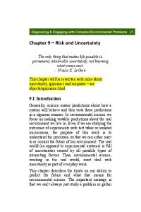
CHAPTER TWO: LEARNING ON THE JOB, A CASE STUDY INTRODUCTION This chapter presents the results of a case study initiated as part of this research. It begins with the identification of the basic elements of the case study. These elements will be of interest to all readers. Next, the chapter offers an overview introduction to the Habitat Evaluation Procedures (HEP) of the Department of the Interior’s Fish and Wildlife Service (U.S. Fish and Wildlife Service) using the rainbow trout model as an example. Those familiar with the HEP analysis technique may safely skip this material. A brief description of the conduct of the case study precedes the presentation of the study results which include a deterministic estimate of project outputs, a sensitivity analysis, and a preliminary risk-based analysis of project outputs. The case study provided enough lessons learned so that when they were combined with what is already known about risk analysis, they formed the basis for the procedures presented in this manual. This makes the case study a valuable lesson for anyone who might venture into risk analysis of ecosystem restoration projects. IDENTIFYING A CASE STUDY A nationwide search of Section 1135 studies was conducted by the Institute for Water Resources (IWR) in order to identify a case study for this research effort. Several candidate studies were identified. The selection criteria were basic: the study’s habitat evaluation work had to be completed within a time frame compatible with this research and the District had to be willing to offer their study as a case study. This latter criterion is not an insignificant one. It is not easy to invite people in to look over your shoulder and to use your work as an object lesson for others. Thus, in appreciation for the District’s cooperation in this research, the actual case study will remain anonymous, although actual events will be described and real data will be used throughout the case study. The case study is called the Brown Sugar River and Sympathy Lake HEP Analysis. PROJECT BACKGROUND Other than the name changes, the description that follows is real. Sympathy Lake is located 85 miles southeast of a major city on the Brown Sugar River about 12.8 miles above its confluence with the Midnight River. Brown Sugar River once supported a warm water fishery. After the construction of Tentshow Dam, the warm water fishery was adversely impacted by cold water releases from the dam for the generation of hydroelectric power. Re-establishment of the warm water fishery was not considered feasible and in the 1950s the State Conservation Department began to introduce a cold water fish, the rainbow trout, to the Brown Sugar River downstream of the dam. This was done in response to intense public interest in a fishery to replace the warm water fishery. Figure 1 provides a stylized map of the project area. A year-round cold water fishery could not be established because of low dissolved oxygen (DO) levels that occur in the summer and early fall months along the lower Brown Sugar River. During these months, Sympathy Lake becomes thermally stratified with very low DO levels in the hypolimnion. Because the hydropower intakes are located at the lower elevations of the reservoir, the low DO hypolimnetic water is released into the Brown Sugar River below the dam.

5

Risk and Uncertainty Analysis Procedures for the Evaluation of Environmental Outputs

Figure 1: Map of Project Area Sympathy Lake

Labyrinth Weir

Tentshow Dam

Midnight River

Brown Sugar River

Various studies have shown that low DO levels combined with lack of flow affect the survivability of the downstream trout fishery. In addition, these conditions also adversely affect the benthic community, which is a major component of the food chain for the river’s aquatic community. As a result, there is little or no growth in the trout stocked in the river and there is little evidence that trout survive beyond the stocking year. Despite a reservoir release program, trout losses still occur. The District has proposed construction of a labyrinth-shaped weir spanning 242 feet of river about 2,000 feet downstream of Tentshow Dam. The zig-zag configuration of the weir would result in an overall length of about 2,100 feet. The crest would be about 3.5 feet above normal water surface during power generation. Water would flow over the weir crest at a depth of about 6 inches, creating a head differential across the weir of about 4 feet. Pipes would be installed in the weir to allow low flow releases from the weir. The weir would be constructed of treated timber stop logs that could be removed for emergencies. The weir is expected to address both the DO and low flow problems that have restricted the cold water fishery. It would cost about $3.35 million to construct and $1,000 annually to operate. The primary benefit of the project would be a more viable cold water fishery.2 There are eight alternative plans under consideration. For simplicity, the alternatives will be numbered 1 through 8 and they are summarized in Table 1. They all include the labyrinth-shaped weir. The 25 cubic feet per second (CFS) flow for Plan 1 is leakage from the dam. The alternatives differ by the

2

Improving the habitat for a non-indigenous recreational fishery is not uncommon among Section 1135 projects. Nonetheless, the restoration of ecosystems via the Section 1135 program can encompass far more varied and complex planning objectives.

6

Risk and Uncertainty Analysis Procedures for the Evaluation of Environmental Outputs

Table 1: Brown Sugar River Sympathy Lake Alternative Plans Plan Number

Labyrinth Weir

Minimum Flow (cfs)

Pulses on Weekend

1

Yes

None (25 cfs)

None

2

Yes

100 cfs

None

3

Yes

75 cfs

None

4

Yes

75 cfs

1 hr. at 4 PM

5

Yes

75 cfs

1 hr. at noon

6

Yes

50 cfs

None

7

Yes

50 cfs

1 hr. at 4 PM

8

Yes

50 cfs

2 hr. at 3 PM

presence and extent of a minimum flow and whether water is released in pulses on the weekend from Tentshow Dam. Plans 3, 4, and 5 are based on a two-day weekend. Plans 6, 7, and 8 are based on three-day weekends. The weir is considered to provide most of the desired DO effects. The minimum flows and pulses affect water temperature. HABITAT EVALUATION METHODOLOGIES Ecosystem function is difficult to describe and measure. Habitat is one ecological resource that is commonly used to represent ecosystem function. In general, more habitat is assumed to indicate better ecosystem function. Thus, habitat improvements are commonly used as surrogate measures of ecosystem restoration project outputs. Habitat can be improved in two basic ways. There can be an increase in the amount of habitat available or there can be improvement in the quality of the habitat available. Increases in the quantity and quality of habitat are also possible. Because there can be many different kinds of habitat in an ecosystem, a problem arises in describing habitat improvements. How do we describe such complex concepts in a compact yet serviceable way? Although many options are available it is common practice to identify a few key species from an ecosystem and discuss the changes in their habitats. The presumption is that if the species are carefully chosen in a representative manner this can reasonably serve as an indicator of the overall ecosystem function. For example, if a species at the top of the food chain is doing well, chances are good that the species below it in the food chain are also doing well.

Changes in the habitats of these indicator species are frequently measured in habitat units for the more common and less complex ecosystem restoration studies. A habitat unit is a theoretical indicator that combines the quantity and quality dimensions of a habitat in a simple mathematical way.

7

Risk and Uncertainty Analysis Procedures for the Evaluation of Environmental Outputs

Habitat quantity is estimated as some physical quantity of terrestrial or aquatic habitat, usually acres. Habitat quality or suitability, however, is quantified via an index number between zero and one. An index of one indicates the habitat in question is optimal for the specific indicator species under consideration. An index of zero indicates very poor habitat. Intermediate values might indicate average habitat conditions, and so on. Changes in habitat units can be used to represent the ecological impacts of habitat unit activities or planned improvements. For example, suppose we have 10 acres of land with an average suitability index of 0.6. Such land would yield 6 habitat units: (1) 10 acres x 0.6 = 6.0 habitat units Now suppose an ecosystem restoration plan would double the acres of habitat and increase their quality from 0.6 to 0.8. The result would be 16 habitat units: (2) 20 acres x 0.8 = 16 habitat units The plan would result in a net output of 10 additional (16 habitat units with the plan minus 6 habitat units without the plan) habitat units. The increase of 10 habitat units is used to represent an improvement in overall ecosystem function. The true change in ecosystem function is usually far more complex and much more difficult to describe, much less to quantify. Until science is better able to describe and quantify ecosystem function in a cost-effective manner, the use of surrogate measures like habitat units will remain a viable tool in decision-making. There are many methods for estimating ecosystem function improvements in this general way. The process is much more an art than it is a science at this point in time. Analysts can choose from among many methodologies that rely on some variation of this quantity times quality approach to quantifying ecological outputs. The procedures developed in this manual are applicable to most of these methodologies. To illustrate the use of the procedures, however, the Habitat Evaluation Procedures methodology of the U.S. Fish and Wildlife Service has been selected. It was chosen because it is believed to be the methodology in widest use in the Corps’ ecological restoration studies at this time. HABITAT EVALUATION PROCEDURES OF THE U.S. FISH AND WILDLIFE SERVICE The philosophy and theory behind the HEP of the U.S. Fish and Wildlife Service are described at length in two Ecological Service Manuals produced by U.S. Fish and Wildlife Service. These are: Habitat as a Basis for Environmental Assessment, 101 ESM and Habitat Evaluation Procedures (HEP), ESM 102. This section provides a brief introduction to the HEP method of developing the index number used to represent habitat quality. The HEP analysis index number is called the habitat suitability index (HSI). The estimation of a habitat unit in an HEP analysis can be formally defined as: (3a) Quantity x Quality = Habitat Units (3b) Acres x Habitat Suitability Index = Habitat Units

8

Risk and Uncertainty Analysis Procedures for the Evaluation of Environmental Outputs

An HSI conceptually reflects the overall suitability of an area of water or land for a particular indicator species. Information for estimating habitat suitability for a specific species can be found in a habitat suitability model description published by the U.S. Fish and Wildlife Service. For example, the next section describes the Habitat Suitability Information: Rainbow Trout, January 1984. In general a habitat suitability model reviews the scientific literature pertaining to the species of interest. From this literature review a set of habitat variables is identified. These variables describe those environmental factors that are important to the survival, growth and reproduction of the species. For the rainbow trout, 18 habitat variables (labeled V1 through V18) were identified. They included things like the average maximum water temperature (EC) during the warmest period of the year and the average velocity (cm/sec) over spawning areas during embryo development. The suitability of a given habitat is evaluated in terms of each of the relevant habitat variables by means of a suitability index (SI). A suitability index graph for the rainbow trout is shown at Figure 2. The curves were built on the assumption that increments of the habitat variable plotted on the x-axis could be directly converted into an index of suitability from 0.0 to 1.0 for the species. Thus, the SI number is at best a science-based subjective judgment on the part of the authors of the HSI model.

Figure 2: Sample Suitability Index Graph 1

Suitability Index

0.9 0.8 0.7 0.6 0.5 0.4 0.3 0.2 0.1 0

0

5

10 Percent

15

20

Variable 8: Percent substrate size class (10 to 40 cm) used for winter escape cover.

The example in Figure 2 shows that when the percent of substrate in the 10-40 cm size group is zero, the habitat is lacking in escape cover for fry and small juveniles. Unlike an HSI of zero, an SI of zero need not imply the habitat is totally unsuitable for the species. The overall suitability of the habitat as reflected by the HSI reflects a composite trade-off of the relative strengths and weaknesses of the habitat’s various characteristics.

9

Risk and Uncertainty Analysis Procedures for the Evaluation of Environmental Outputs

The various habitat variables are grouped into “components” that are sometimes called “life requisites.” For example, the rainbow trout has a fry component (CF), an embryo component (CE), a juvenile component (CJ), an adult component (CA), and an other component (CO) that can be subdivided into food (COF) and water quality (COQ) components. These components are mathematical combinations of the SI’s for the various habitat variables that define that component. Component values are also index numbers between zero and one. For example, the food component for trout is defined as follows:

(4)

COF '

(V9 x V16).5 % V11 2

where V9 is predominant substrate type in riffle-run areas for food production; V16 is percent fines in riffle-run areas during average summer flows; and, V11 is average percent vegetational ground cover and canopy closure along the streambank for allochthonous input. Suppose, for example, the SI’s for each of these variables are V9 = .5, V11 = .6, and V16 = .7. Then the value of COF would be 0.596, say 0.6. Model components are calculated in a similar fashion for each model component. The model components are then used to produce an HSI. Thus, the general progression of an HSI model is: (5) Habitat variable measurements => Suitability indices => Component indices => Habitat suitability index One of the most common methods for estimating an HSI is to use the minimum component value from among the relevant component values for a particular model. Another common HSI estimating algorithm is to multiply the components together and take the root equal to the number of components. For example, if there are three components you might use the cube root of the product of the three component values. Before considering the trout model more specifically, it bears repeating that this evaluation technique may be science-based, but it is fundamentally a subjective art. Analysts routinely adapt the HSI models to local conditions and needs. For example, because the rainbow trout is not an indigenous species in the case study area, the river is stocked annually and no attempt is made to establish a breeding trout fishery. In this case, there is no need for embryo, fry, or juvenile components in estimating the HSI for the project area. RAINBOW TROUT HABITAT SUITABILITY INDEX MODEL Habitat Suitability Index: Rainbow Trout was prepared by Robert F. Raleigh, Terry Hickman, R. Charles Solomon, and Patrick C. Nelson in January 1984 as report FWS/OBS-82/10.60. The model, like most, begins with a review of the scientific literature that summarizes what is known about the rainbow trout. The overall structure of the model is presented in Figure 3. As described above, it shows habitat variables feeding into model components that subsequently feed into the HSI.

10

Figure 3: Rainbow Trout HSI Model Habitat Variables Avg. thalweg depth (V4) % instream cover (V6A) % pools (V10) Pool class rating (V15) % instream cover (V6J) % pools (V10) Pool class rating (V15) % substrate size class (V8) % pools (V10) % riffle fines (V16B) Avg. max. temp. (V2) Avg. min. D.O. (V3) Avg. water velocity (V5) Avg. gravel size in spawning areas (V7) % riffle fines (V16A) Max. temperature (V1) Avg. min. D.O. (V3) pH (V13) Avg. base flow (V14) Predominant substrate type (V9) % streamside vegetation (V11) % riffle fines (V16B) % streamside vegetation (erosion) (V12) % midday shade (V17) % avg. daily flow (V18)

Model Components

Adult

Juvenile

Fry

HSI Embryo

Other

Risk and Uncertainty Analysis Procedures for the Evaluation of Environmental Outputs

The model itself is divided into lacustrine and riverine habitats for the trout. In this case study, the goal was to improve the riverine habitat for adult trout. This did not require a model with all the complexity shown in Figure 3. The model actually used was an adaptation of this model and it is shown at Figure 4.

Figure 4: Modified Rainbow Trout HSI Model Habitat Variables Avg. thalweg depth (V4) % instream cover (V6A) % pools (V10) Pool class rating (V15) Max. temperature (V1) Avg. min. D.O. (V3) pH (V13) Avg. base flow (V14) Predominant substrate type (V9) % streamside vegetation (V11) % riffle fines (V16B) % streamside vegetation (erosion) (V12) % midday shade (V17)

Model Component

Adult

HSI

Other

To aid the reader unfamiliar with HEP analysis, let’s take a look at two habitat variables that will be of particular interest later in this manual. The first is V1, average maximum water temperature (EC) during the warmest period of the year. Its suitability index graph is shown at Figure 5. The second variable is average minimum dissolved oxygen (mg/l) during the late growing season low water period and during embryo development (V3). It’s suitability index graph is shown at Figure 6. The District’s field team estimated V1 for one reach to be 23.9 EC with a corresponding SI= .25. V3 was estimated to be 0 mg/l with a corresponding SI of 0. In a similar fashion, using the suitability index graph, a measurement for every variable estimated in the field was converted to a corresponding SI value. The SI values were used to estimate values for the model components. The model components values, in turn, were used to estimate the HSI. BROWN SUGAR RIVER AND SYMPATHY LAKE CASE STUDY INTRODUCTION The authors want to thank, without naming, the cooperating District and its personnel who so generously gave their time and cooperation in this research effort. This manual would not have been possible without their cooperation.

12

Risk and Uncertainty Analysis Procedures for the Evaluation of Environmental Outputs

Figure 5: Water Temperature Suitability Index Graph Suitability Index

1 0.9 0.8 0.7 0.6 0.5 0.4 0.3 0.2 0.1 0

0

2

4

6

8

10

12 14 16 18 20 Degrees Centigrade

22

24

26

28

30

Average maximum water temperature during the warmest period of the year

Figure 6: DO Suitability Index Graph 1

Suitability Index

0.9 0.8 0.7 0.6 0.5 0.4 0.3 0.2 0.1 0

3

3.5

4

4.5

5

5.5

6 mg/l

6.5

7

7.5

8

8.5

9

Average minimum dissolved oxygen (mg/l) during the late growing season low water period.

13

Risk and Uncertainty Analysis Procedures for the Evaluation of Environmental Outputs

PREPARATION Identification of the Brown Sugar River and Sympathy Lake project as a feasible case study took a considerable amount of time and it offered a rather narrow window of opportunity. Two researchers for this project joined District personnel for the first time the morning that the HEP analysis field data were to be collected. Following an introduction to the project by the project manager, the researchers gave a brief overview of this research effort and the purpose and methods of risk analysis. By mid-morning, all were en route to the project site. FIELD DATA COLLECTION The District contracted the HEP analysis to the U.S. Fish and Wildlife Service. The field team gathered along the banks of the Brown Sugar River at an access point just downstream of the proposed weir site below the Tentshow Dam. The rainbow trout, channel catfish, and largemouth bass had been previously identified as the suite of indicator species that would be used for the HEP analysis. A standardized form listing all the habitat variables required to conduct HEP analyses for these three species was prepared in advance of the site visit. Organizing the set of variables on a single form eliminated the redundancy that would have resulted had the team done a species-by-species evaluation. Initial estimates of habitat variables were the point estimates (e.g, 80% streamside vegetation (V11)) to which these experts had been accustomed. With an explanation and occasional prodding, they were willing to estimate some, but not all, of the habitat variables as intervals (e.g, 70-90% streamside vegetation (V11 )). There was not enough budget to make many field measurements using instruments, although oxygen, temperature, pH, and flow measurements were taken at each of four data gathering points. Data for these four variables were to be supplemented with previously collected measurements. There seemed to be a certain amount of discomfort with the notion of using intervals to estimate habitat variable values. The team gathered at a single access point along the river at which it was possible to see perhaps 200 yards upstream and downstream of the access point. Estimates of habitat variable conditions made at this location were used to represent 1.55 miles of river. Subsequent single access points, with roughly similar visibility, were used to estimate habitat variable conditions over reaches of 2.23 miles, 2.92 miles, and 1.00 mile of river. Despite the fact that only a small portion of the river was visible and most estimates were subjective, the team generally estimated a relatively small range of variation in conditions, when a range was estimated at all. For example, consider trout habitat variable V6, “percent instream cover during the late growing season low water period at depths $ 15 cm and velocities < 15 cm/sec.” Initial estimates at the first access point were that this would average about 3 percent over the 1.55 miles of river. When the team discussed the variation in cover visible from its location and possible variations over the stretch of river not visible to the team, all agreed there was some uncertainty. An interval estimate of from 2 to 5 percent replaced the point estimate of 3 percent. The range of uncertainty expressed by the team was often limited when the actual uncertainties seemed to be potentially much greater. The percent of midday shade, for example, was estimated to range from 1 to 2 percent. The habitat variable measurements collected by the field team are presented in Appendix 1.

14

Risk and Uncertainty Analysis Procedures for the Evaluation of Environmental Outputs

DISTRICT HEP ANALYSIS About $9,000 had been budgeted to the U.S. Fish and Wildlife Service for this HEP analysis for this purpose. The results of this analysis are summarized in Table 2. There are eight plans, each addressing three indicator species along four reaches. That results in 12 sets of HSI’s without the project, 96 HSI’s with the project, yielding 108 sets of habitat unit values, as well as 96 changes in habitat units3. For simplicity, only the change in habitat unit results for two plans are reported here. The detail on the individual species and reaches has been collapsed into to a single value, so as not to drown the reader in details.

Table 2: Change in Habitat Units for Plans 1 and 2 Plan

1

2

Habitat Unit Increase

74.89

143.21

The values in Table 2 are very precise. It’s clear that Plan 2 results in the greatest increase in habitat units for all species and all locations. But are these numbers as accurate as they are precise? These are the numbers that are typically provided to decision-makers. Numbers like these may lead Corps officials, State and Federal resource agency personnel, and the public to believe that the outputs of this project are far more certain than they in fact are. As the next chapter will reveal in detail, there is good reason to think they are not as accurate as they are often thought to be. Okay, you might say, suppose these estimates are not exact. Is that important? Does it make a difference? Suppose the actual habitat improvements do vary some from these estimates. If you concede that point, the important question then becomes, “What do we mean by “some”?” Are we likely to be off by one habitat unit or 100 habitat units? One habitat unit may make no difference at all, but 100 habitat units may be the difference between saying yes or no to the project. And if it could be off by 100 habitat units, how likely is it to be off by that much? Is that a one-in-a-million chance or is it a 50/50 proposition? These are important questions. If decision-makers have no information to help answer them, they could make a bad decision about a project. The best alternative might not be chosen. Scarce resources might be directed to a bad project rather than to a good one. These questions can’t be answered unless they are specifically investigated. The certainty of an outcome is as subject to investigation as hydrology, foundation conditions, or any other detail of a project is. Risk analysis is the broad name given to the collection of methods by which such questions can be addressed. One tool of risk analysis is sensitivity analysis. Sensitivity analysis requires the analyst to define different analytical scenarios. The calculation of habitat units is repeated for each scenario. Significant differences in results can then be attributed to the differences among the scenarios. In sensitivity analysis, the analyst systematically changes the value of selected elements of the analysis and recalculates the results. If the

3

Each alternative plan has the same without project condition. Because there are three species and four sites there are 12 different sets of HSI’s without the project. The with project condition varies for each plan so 8 x 12 yields the 96 with project condition sets of HSI’s.

15

Risk and Uncertainty Analysis Procedures for the Evaluation of Environmental Outputs

change in the result, when compared to the best estimate or base measure, is insignificant then you can be confident that the value that was systematically changed will have no material influence on the outcome. For example, suppose the thalweg depth in our best estimate of the change in habitat units for rainbow trout is 61 cm. Suppose there is some possibility the thalweg depth is as much as 122 cm. In a sensitivity analysis, we would change this value to 122 cm and recalculate the change in habitat units. The change in thalweg depth would have no impact on the change in habitat units because any value over 45 cm in depth is optimal for trout as Figure 7 shows. Therefore, we can say with complete confidence in this instance, that the difference in thalweg depths under consideration (i.e., 61-122cm) will have no impact on our decision. On the other hand, there may be uncertainty about another habitat variable that makes a significant difference for this project. Sensitivity analysis is a simple but valuable tool for introducing risk analysis into a study.

Figure 7: Thalweg Depth Suitability Index Graph 1

Suitability Index

0.9 0.8 0.7 0.6 0.5 0.4 0.3 0.2 0.1 0

0

5

10

15

20

25 30 35 40 Thalweg Depth (cm)

45

50

55

60

Average thalweg depth (cm) during the late growing season low water period.

As a result of the desire to incorporate some risk analysis into the evaluation of ecosystem restoration projects, U.S. Fish and Wildlife Service personnel did some sensitivity analysis using the ranges of variable values estimated in the field. The values in Table 3 reflect some uncertainty in the potential outputs of the plans. There is a 20 to 30 percent variation in project outputs using this simple sensitivity analysis. Any number of scenarios can be investigated in a sensitivity analysis. Perhaps the most common set of scenarios include the most likely condition as well as the worst and best case scenarios. Worst and best case scenarios should represent the worst and best possible outcomes that are reasonably foreseeable. That is, they are not simply a bad outcome and a good outcome. In some situations, pessimistic and optimistic scenarios are used to represent bad and good outcomes that are not necessarily the extreme

16

Risk and Uncertainty Analysis Procedures for the Evaluation of Environmental Outputs

Table 3: District Sensitivity Analysis for Selected Plans Plan

1

2

Pessimistic Scenario Habitat Unit Increase

58.44

117.62

Most Likely Scenario Habitat Unit Increase

65.51

130.06

Optimistic Scenario Habitat Unit Increase

74.89

143.21

scenarios represented by a worst and best case analysis. The U.S. Fish and Wildlife Service used their own scenarios to produce pessimistic and optimistic scenarios. RISK-BASED HEP ANALYSIS In an effort to demonstrate the feasibility of incorporating risk analysis into the habitat evaluation portion of a study, the data collected by the field team were used to build a model that simulates the range of results using a Monte Carlo process. The results shown in Table 4 do not vary too much from the sensitivity analysis.

Table 4: Selected Results of Risk-Based Estimate of Habitat Unit Increases Plan

1

2

Minimum Habitat Unit Increase

71.23

89.23

Mean Habitat Unit Increase

73.02

96.44

Maximum Habitat Unit Increase

74.66

100.07

Briefly, the Monte Carlo simulation (discussed in more detail in Chapters Five and Six), used the same ranges of habitat variables that the District used in its sensitivity analysis. These ranges are shown in Appendix 1. With a Monte Carlo process variable values are selected at random from the ranges of habitat variable values (according to some prescribed probability distribution) and the HSI’s and HU’s are computed. This process is repeated a large number of times, in this case 4,000 times. Thus, instead of two extreme value estimates, the Monte Carlo process generated a distribution of 4,000 values. Selected outcomes of the simulation are presented in Table 4. The extreme values shown in Table 4 differ from those in Table 3 primarily because the event of all habitat variable values was to rare to be observed in a simulation of 4,000 iterations. Presumably, a simulation with many thousands more iterations would eventually reproduce the extreme values of the sensitivity analysis

17

Risk and Uncertainty Analysis Procedures for the Evaluation of Environmental Outputs

along with an estimate of the probability with which those extreme values are likely to occur4. Most likely and mean values differ because the distributions assumed for the Monte Carlo simulation resulted in expected values that sometimes differed from the most likely value used for the sensitivity analysis. SUMMARY AND LOOK FORWARD The case study used for this manual and the basics of HEP analysis were introduced in this chapter. Field experience demonstrated the feasibility of estimating habitat variables as intervals rather than as points. Agency personnel used the interval estimates to produce a simple sensitivity analysis within the original study budget and schedule. The same values were then used in a Monte Carlo simulation to estimate project outputs. Thus, two primary risk-analysis tools are introduced in this chapter. The results presented in this chapter clearly demonstrate the feasibility of conducting risk-based analysis within the budgets and schedules of simple Section 1135 investigations. The next chapter considers some of the important lessons that were learned from this case study.

4

For example, suppose a simulation of 100,000 iterations was run and the extreme values of Table 3 showed up once each. We could then estimate the probability of these extreme values to be 0.00001 or 1-in-100,000. Thus, a simulation adds a powerful dimension to our analysis of potential outcomes, i.e. estimate s of their likelihood of occurrence. These details will be explored in later chapters.

18

Risk and Uncertainty Analysis Procedures for the Evaluation of Environmental Outputs

CHAPTER THREE: LESSONS LEARNED INTRODUCTION Most ecosystem restoration studies rely on single-valued, deterministic results as the basis for major decisions. The professional integrity of the organizations and individuals doing the analysis is usually sufficient justification for accepting the results. Risk and uncertainty analysis, while it moves away from single-valued deterministic analysis, is not a challenge to anyone’s integrity or professional judgment. Risk analysis simply recognizes the realities of a complex and often difficult world and offers a systematic approach for investigating and considering key uncertainties in the decision-making process when warranted. The procedures offered in Chapter Four find their genesis in the lessons learned from the case study of the previous chapter. This chapter discusses the lessons learned. The next chapter combines the lessons learned with experience gained by the risk analysis community over the years, to develop some generic risk analysis procedures for ecosystem restoration projects. Although some of the lessons learned in the case study may represent new insights, most of them are confirmations of common situations that arise. If you are involved in risk-based habitat evaluation work, be prepared to address these concerns, because they are that common. Be forewarned that you can expect problems not addressed here to arise as well. The lessons learned have been organized into three sections. First, there are lessons learned about how to prepare for a risk-based habitat evaluation analysis. Second, there are lesson learned about data collection. Finally, there are the lessons learned while conducting the analysis. PREPARATION Perhaps the number one lesson learned is that preparation is the most important phase of a risk-based analysis. If people do not understand what uncertainty is or that it must be addressed, all else is futile. If the reasons for addressing this uncertainty are not clear to analysts, there is going to be little enthusiasm for the analysis and little hope that it will be done well. Thus, we begin with the lessons that must be learned before analysis begins. REALIZE THAT UNCERTAINTY EXISTS What are “with project” conditions going to be? Will an increased stream flow lower temperatures? If so, by how much? Could the flows affect DO as well? By how much? Will the flows have any impact on stream velocities? How much of an impact will these changes in water quality really have on the rainbow trout or channel catfish? You may have some ideas about the answers, maybe some pretty good ones. But the truth is, we don’t know for sure. We’re uncertain. Virtually all “with project” condition forecasts are uncertain. The same thing goes for “without project” forecasts. Will DO levels stay the same or are there processes at work in the reservoir that will result in more or less DO in the water released for hydropower in the years ahead? Forecasts are by their nature uncertain. Even getting good estimates of complex variables that are right in front of you, when you have only a few minutes to estimate them, is impossible to do with certainty. Uncertainty is present in all steps and iterations of the planning process. It is especially rampant in ecosystem restoration planning.

19

Risk and Uncertainty Analysis Procedures for the Evaluation of Environmental Outputs

Getting people to acknowledge the existence of uncertainty is going to be one of the greatest obstacles to incorporating risk analysis into ecosystem restoration. Ecosystem restoration analysts are likely to be faced with daunting tasks and constraints on their time, budgets, personnel and capabilities. Although they are laboring in the face of substantial uncertainties they often have neither the time, training nor inclination to consider that uncertainty in anything more than the most cursory fashion, if they consider it at all. Analysts who already feel they have more to do than can possibly be done well with the available resources may not be well disposed toward taking on the additional analytical and deliberative responsibilities that risk analysis represents to them. The first step must always be to get the study participants (planners, partners, and public) to realize that uncertainty exists and it is natural, expected and unavoidable. Next, they must understand that some uncertainties might substantially affect the alternatives they formulate or the performance of the alternative they select in such a way that the important decisions they are called on to make could change significantly. For example, if DO is 0 mg/l you will definitely be steered toward alternatives that increase DO. But if DO is really closer to 6 mg/l, then low flow conditions might be more important and your choice of actions could be substantially different. The first goal in any risk analysis must always be to get people to see that: 1) uncertainty exists and it is unavoidable; and 2) some uncertainties could materially affect your decisions. When the first goal is accomplished, the second goal is to address the important uncertainty in your study. UNDERSTAND UNCERTAINTY AND LEARN HOW TO THINK ABOUT IT Once planners and others are aware of the existence of uncertainty in a general sense and the potential significance of important uncertainties, the next step is to learn how to think about the nature of uncertainty. Chapter Three of the March 1996 IWR Report 96-R-8 An Introduction to Risk and Uncertainty in the Evaluation of Environmental Investments provides a good introduction to the basics of risk and uncertainty analysis. It is important to understand the kinds of things that can be uncertain (theory and knowledge, models, and quantities) and the sources of that uncertainty (random error and statistical variation, systematic error and subjective judgment, linguistic imprecision, variability, randomness and unpredictability, disagreement, and approximation). This manual places a good bit of emphasis on the uncertainty that arises because of variability among elements of a population. This is a common source of uncertainty in ecosystem restoration projects. But it must be emphasized that this is not the only source of uncertainty that arises in these projects. Nor will it always be the most important source of uncertainty. In order to design and conduct a good risk analysis, analysts need a systematic way to approach their work. The taxonomy of IWR Report 96-R-8, taken from Morgan and Henrion (1990), offers such an approach. PURPOSE OF RISK ANALYSIS The purpose of risk analysis is to improve the quality of the decisions being made in ecosystem restoration studies. That happens when the analysis enables the planners to tell stakeholders and decision-makers what is known, what is not known, and what is partially known about problems and their solutions. Armed with this heretofore missing dimension of the information they are working with, decision-makers will be better informed. Better informed decision-makers should make better decisions. IDENTIFY THE MAJOR UNCERTAINTIES 20

Risk and Uncertainty Analysis Procedures for the Evaluation of Environmental Outputs

Truth be told, in an ecosystem restoration project virtually everything is uncertain to some degree. The purpose of risk analysis is not to cripple the study with the burdens of additional time, budget, or resource requirements, just to be able to say a risk analysis was done. The sole purpose of a risk-based analysis is to improve the quality of decisions made. Those decisions include the formulation of alternatives, evaluation and assessment of their impacts, comparisons of alternatives, and the final recommendation of the study. If the costs are small, the problems are simple, and the consequences of being wrong are trivial, there may be no need for anything more than a cursory and subjective risk analysis. For example, one might say the outputs of Plan A are more certain than the outputs of Plan B. In other cases, a more detailed analysis is required. In either case, it is important to focus the analysis on uncertainties that matter to the decision process. An example of important uncertainties are those that create important differences in the estimation of project effects that could influence the formulation of alternatives or the choice from among them. In the case study, DO was identified by many parties as the most important limiting factor in the ecosystem. A low DO level was identified as the reason a cold water fishery had not been successfully established. Although the actual DO level was not known with certainty, this variable was treated as a deterministic value by the field team, even in the sensitivity analysis and simulation of the preceding chapter. In general, an analysis should not treat such an important variable as deterministic unless it in fact is deterministic. On the other hand, there are habitat variables that simply are not important in a given situation because they are not constraining the ecosystem. An example would be the thalweg depth as discussed in the last chapter. Depths in excess of 45 cm yield a suitability index of 1. In the case study, this value was allowed to range from 61 to 122 cm. Despite this relatively substantial range in thalweg depths, it had absolutely no impact on the HSI estimation, estimates of project outputs, or the formulation process. It was not a constraining variable and although the average thalweg depth is indeed uncertain, it is not an important uncertainty. It need not be considered because it will have no effect on the study decision. Ignore the uncertainties that are not important, but be sure they are unimportant before you ignore them. Which habitat variables are important and which are not will vary from species-to-species and from study-to-study. In a related fashion, which uncertainties are important and which are not is going to vary from situation-to-situation. What will not vary is the importance of concentrating only on those uncertainties that are important; i.e., the ones that have the potential to result in the formulation or selection of different alternatives. Spend time before collecting data identifying and discussing the major uncertainties. These discussions would ideally involve all the stakeholders in the study process.

21

Risk and Uncertainty Analysis Procedures for the Evaluation of Environmental Outputs

CLARIFY YOUR LANGUAGE Language can be a concealed, yet serious, source of uncertainty. Read an HSI model and we all have a pretty good idea of what the familiar terms mean. I know a pool when I see one, I know what shade is, I understand what a river bank is. These terms are common, everyday English. But when you get out in the field with a group of people, it is amazing how divergent people’s views are on what constitutes a pool, shade, or a bank. It is impossible to generate a consensus estimate of the percentage of pools if we each think of a pool as something different. It is important to take the time to clarify what is meant by the words you use. Pay particular attention to the terminology used in models prepared by others. When there are many points of view, it may be less important which will be used than that everyone have a common and accurate understanding of what the terms used mean. Clearly, when the terms are important because of their use in a source document like an HSI model, the prevailing definition should be that of the authors of the model whenever possible. Consistency is important. It is essential that everyone use the same definition. PREPARATION IS IMPORTANT Being prepared to do a risk analysis is an essential part of doing a good risk analysis. That means analysts must recognize not only the existence of uncertainty but also the value of dealing with major uncertainties explicitly. This takes a great deal of effort the first time or two risk analysis is used by a person or study team. It is during these times that people must learn the basics of risk and uncertainty analysis. What is it, why is it important, how can I deal with it? Potential tools are discussed in Chapter Five. Unfortunately, the answers to these questions require effort on the planner’s part. Fortunately, once that effort is expended it need not be expended again. Instead it can be built upon. DATA COLLECTION Once you have prepared for a risk analysis it is important that data be collected in a fashion that will support risk analysis. Some lessons learned about data collection follow. DEVELOP GROUND RULES FOR DATA COLLECTION Ask a group of people a question that has a subjective answer and you are likely to get a bunch of different answers. The range of answers reflects the uncertainty inherent in the situation. It can be very helpful in addressing the uncertainty in a situation to develop a set of ground rules that will help identify the uncertainty inherent in a situation. Before data collection begins, the team should develop and agree to a set of ground rules that will dictate how the data collection will proceed. The purposes of the rules are to ensure everyone that their efforts will be considered and to work out a procedure by which the work will be accomplished and model values determined. The rules can vary from situation-to-situation. They might be as simple as, “The U.S. Fish and Wildlife Service personnel will do the analysis as they see fit.” If an interdisciplinary or inter-agency team is used, however, it may be helpful to develop and agree to rules that make sense for the situation. A few generic suggestions follow: 22

Risk and Uncertainty Analysis Procedures for the Evaluation of Environmental Outputs

1.

Indicator species will be identified well in advance of the field work.

2.

Everyone shall read the HSI model (or appropriate background material if other techniques are used) prior to the field work.

3.

The data team, working in a group session, will review each habitat variable to be measured to ensure a common definition of all terminology prior to beginning data collection.

4.

In the event of differences of opinion on the meaning of any terms the judgment of (provide your decision rule here) the majority/project manager/U.S. Fish and Wildlife Service/chief environmentalist shall prevail.

5.

All field measurements will be taken at least twice and by different people if possible.

6.

Any variable that is measured subjectively will first be estimated silently and independently by each team member. Once all variables have been estimated, each will be discussed in turn to clarify any differences of opinion and to develop consensus values for the variables to be used in any models or analysis.

7.

Preserve the variation in observed values recorded by the team members. These can form the basis for sensitivity analysis, the description of subjective probabilities, or the specification of probability distributions used in your risk analysis.

More ground rules can be developed as necessary. For example, it may be advisable to develop rules for reaching the consensus referenced in item 6 above. If the study calls for a more detailed data collection effort, including a sampling design, then more detailed rules are going to be required. Rules may need to be tailored to the personnel doing the work. Any rules that meet the needs of the study are acceptable. Working out the rules ahead of time, rather than developing them on an ad hoc basis, offers the advantages of prior thought and fairness. Neither of these should be neglected. WORK INDEPENDENTLY AT FIRST One opinionated or authoritative person can dominate the position of a group. If that one person is unaware of, denies or underestimates the existence of uncertainty in a situation the analysis may not address uncertainty as well as it might. If the extent of the uncertainty is going to be fully explored, it’s going to take the best efforts of everyone involved in the analysis. Thus, it’s important to avoid having any one individual dominate the field data team. One way to do that is to have everyone work on their own at first.

23

Risk and Uncertainty Analysis Procedures for the Evaluation of Environmental Outputs

Data collection efforts are often team efforts. The advantage of a team is that two heads are better than one. To reap the benefits of teamwork, you want to make sure you provide an opportunity for all team members to contribute to the best of their abilities. That means you want everyone to be involved and you want everyone’s effort to be appropriately considered. A common problem that arises in team efforts is the dominant individual. A person may “dominate” a group by virtue of their expertise, size, age, argumentativeness, position of authority, or by other means. When people acquiesce to the opinion of another, either without having first thought through their own opinions or without being truly convinced of the correctness of the other person’s opinion, we have domination. A group can be dominated by the active efforts of the “dominator” or by the passive efforts of the “dominated.” By allowing or requiring team members to initially work individually, you may be able to minimize the dominant individual effect. You’ll also be getting the most from your team’s efforts. The case study field team assembled at the data collection site and began recording values for each habitat variable. After the first couple variables, the entire team settled into its modus operandi which was to have a single dominant individual voice his opinion, only to have everyone else nod their heads in agreement and record what he said. DO, temperature, and pH measurements were taken separately by one team member. Because the team only had time to stop at a single access point for each reach, most of them were completely unfamiliar with the remainder of the river. Because the team yielded to the opinion offered by the dominant individual, the data collection effort was effectively done by one person, despite the presence of the others. This is a situation that should be avoided. It is essential that the field team have a common understanding of all the variables they are trying to measure. This should be assured before data collection begins. Everyone should be encoding the data on identical data collection forms. Everyone should make their own independent estimates of the habitat variable values silently at first. Once all variable values have been encoded for the reach, then the team members should begin to compare their values. Members can offer their reasons for the values they estimated. You may want to allow people an opportunity to modify their own estimates after everyone has offered his rationale. Final decisions about variable values need not, in fact they should not, be made in the field. When dominant individuals might be present, it is best to address this situation in the ground rules established before the work begins. Some rules are offered below for example purposes only: 1) Everyone will record each variable value independently and without discussion with anyone else; 2) Everyone will report the values they recorded, before leaving the data collection site. Everyone is encouraged to offer an explanation for the values they chose; 3) There will be no direct response to anyone’s valuation of a variable. 4) After all results have been reported, everyone will have an opportunity to make any changes to the values they want; 5) The revised values will form the basis for the model values. The lowest and highest values estimated by anyone will become the minimum and maximum values. The average of all most likely values will become the most likely value. As an alternative to this minimum/mean/maximum method, it is perfectly acceptable to make the values of the local expert or anyone else the basis for model values. In that case, other team members play an advisory sort of role in the data collection.

24

Risk and Uncertainty Analysis Procedures for the Evaluation of Environmental Outputs

AVOID USING HEURISTICS TO ADDRESS UNCERTAINTY The biases, imprecision, and overconfidence that usually accompany expert evaluations of things that are fundamentally uncertain provide much of the impetus for uncertainty analysis. If the commonly used point estimates found in habitat evaluation techniques are likely to contain significant errors, then explicit consideration of uncertainty is required to consider possible sources, magnitudes, and implications of these errors. Characterizations of uncertainty are as subject to bias and error as any other scientific analysis. In this section, some important findings from the literature on the psychology of judgment under uncertainty are reviewed. The hope is that once aware of the existence and potential impacts of these heuristics,5 or rules of thumb people often use to address uncertainty, the better you will be able to avoid them in your analysis. The goal is to try to avoid relying on the heuristics that follow. Availability. Experts tend to assign greater probability to events to which they are frequently exposed in the news, media, scientific literature, on their jobs, or in discussion with friends and colleagues. These events are available, in the sense they are easy to imagine or recall. Thus, an expert who has worked repeatedly with a rare situation is likely to think that situation far more likely than it is, in part because of its familiarity to them. Make it a point to consider whether availability might be influencing your estimate of a variable’s value(s). Anchoring and Adjustment. Experts’ estimates of uncertain values are influenced by an initial reference value or anchor, from which they then make adjustments up or down. For example, ask a person how far it is from Denver to Little Rock and a number pops into their head. Then they add some miles to it and subtract some miles from it to get their interval estimate of the distance. They select an anchor and then adjust it up and down. The problem with this kind of response is that the number that pops into an expert’s head may be based on limited experience with a situation or maybe even speculation and incomplete information. Furthermore, the adjustments we make are rarely large enough to reflect the true uncertainty. The result is that our estimates of uncertainty are unduly weighted toward our initial estimate of a value. In practice this means we might look at a river and estimate midday shade at 20 percent. Then we might figure it could be five percent more in either direction. Our estimate is 15 to 25 percent. The estimate is centered around that first value and we perhaps do not appreciate that we could be off by much more than five percent. Challenge your initial response. Representativeness. Experts often judge an event by reference to other events that resemble it. A team stops at an access point and estimates a habitat variable value and figure it is representative of an entire river reach. The problem is that a small sample may carry little or no relevant information about the river reach. Our estimation of population values should not be based on a few values assumed to be typical. Unusual things can happen in small samples.

5

The descriptions that follow have been adapted from The National Research Council’s Understanding Risk: Informing Decisions in a Democratic Society, pp.112-113.

25

Risk and Uncertainty Analysis Procedures for the Evaluation of Environmental Outputs

When forced to use a small sample or a single access point, care must be taken to assure that it is truly representative. If expert opinion is the basis for this judgment of representativeness, bear in mind this is a characteristic that is very difficult to consciously recognize. Thus, at a minimum, it would be useful to explicitly identify and discuss the key variables in your analysis and their conditions at locations that are not visited. Probe the judgment of representativeness. Don’t be too quick to accept the judgment that the entire population or reach is like the little piece of it which you are observing. Belief in “Law of Small Numbers” and Disqualification. Many scientists believe small samples drawn from a population are more representative of the population than can be justified on the basis of statistical sampling theory. In these situations a little evidence, like a single DO reading from a river reach, can unduly influence the analysis. Experts also tend to “disqualify”, i.e, discount or ignore, information that contradicts their opinions. For example, a DO reading that is higher than expected might be explained away as some sort of anomaly. Think about how to appropriately weigh the information you have. Overconfidence. As a result of these and possibly other heuristics, experts tend to underestimate the uncertainty inherent in a given situation. They often overestimate the likelihood that they are correct, or, conversely, they underestimate the possibility that they are wrong. The more difficult and complex the analysis the more likely the overconfidence. It’s not a bad idea to remember experience shows many experts are overconfident. DEVELOP INTERVAL ESTIMATES FOR EVERYTHING It takes very little effort to make or record an interval estimate for field data. Get in the practice of using them for everything you record. Just because you record a variable as an interval estimate, you are not obligated to use it; but it is far better to have it and not use it than to need it and not have it. Remember, intervals almost always increase the accuracy of your work. Most interval estimates are based on expert opinion. Be sure to record a minimum possible value, a maximum possible value, and a most likely value for everything you record. If every member of a team is doing this it will be necessary to combine the results into a single value.6 Be clear on what you mean by “most likely.” The mean is often used when the mode is intended. Whenever possible, it is preferable to take a random sample of variable measurements and develop standard statistical confidence intervals. These can be described, as shown in Chapter Five, as a range of values in which you are, say, 95 percent confident the true value lies, or by specifying the sample statistic estimate and its standard error, if the sampling distribution of the statistic is normal.

6

An alternative to combining the individual results into a team result would be to do a sensitivity analysis and run the analysis using each team member’s results and see if any of them make a difference. For example, suppose it is decided that the U.S. Fish and Wildlife Service estimator’s values will be used and they happen to be different from the Corps estimator’s values. Do the basic analysis using the U.S. Fish and Wildlife Service values, then repeat it using the Corps estimator’s values. If the study results are invariant to the results of this sensitivity analysis then they are of no concern. If the result does vary, then decision-makers must be made aware of the differences or other efforts must be made to address the differences.

26

Risk and Uncertainty Analysis Procedures for the Evaluation of Environmental Outputs

If you find that some team members are not using a range of values to estimate the more subjective values required for your analysis, play the devil’s advocate and challenge the members’ point estimates. Changing the way people think about things will take time. Estimating habitat variables as an interval rather than a point represents a change in the way many of us think about and do things. It will take time and some prodding. Challenge conventional thinking to help people see environmental phenomena in a new light. If you are measuring a variable with meters or other field equipment, take and record multiple measurements and use them accordingly. GET THE RAW DATA WHEN POSSIBLE DO, temperature, pH and streamflow data used in the case study, though measured during the site visit, were taken from prior reports and data collection efforts. Whenever possible, it is desirable to obtain the original or raw data so that you can develop confidence intervals suitable for use in your analysis. UNDERSTAND THE MODELS FOR WHICH YOU ARE COLLECTING DATA It is common sense that analysts should understand the models they use in an analysis. In particular, the analyst should understand the uncertainties inherent in the model and its use. This is not to imply that uncertainties in the models of others need to be corrected or addressed. At a minimum, they should be identified and decision-makers need to be made aware of the situation that exists. The HEP analysis itself is a subjective process that can, at times, be regarded as more scientific than it is because it involves calculations that are very precise if not accurate. The expert knowledge of and experience with the HSI models used in the case study led to the prior preparation of a common data collection form that proved to be very efficient. This was a simple but good example of how understanding the models improved the data collection. GIVE KEY VARIABLES AFFECTED BY PROJECTS SPECIAL ATTENTION The District analysis of the case study assumed that DO without the project was 0 mg/l and with the project it would be 6 mg/l. These were single point estimates of perhaps the most important variable in the entire analysis. If nothing is done, the average minimum DO would be 0. This does not bode well for the rainbow trout or anything else that requires oxygen for life. Nor is it a certainty that this is true, especially because fish do survive in these waters. This meets the definition of a major uncertainty. Likewise, the project is assumed to guarantee an average minimum DO of 6 mg/l. This precision is in spite of the relative novelty of labyrinthshaped weirs. As Chapter Six will reveal, habitat as measured by habitat units is quite sensitive to DO values. Suppose there is more DO without a project than the analysts expect? Suppose the project actually does less for DO than expected? If either or both these situations occur, it’s possible the weir is not a cost-effective way to address the problem. Are either of these situations conceivable? Could they occur together? The answer is yes to both questions. How likely is that to happen? That is a question we cannot answer without some risk-based analysis, as shown in a future chapter. The lesson learned, however, is to make sure you explicitly address the uncertainty in key variables that are going to be affected by a project.

27

Risk and Uncertainty Analysis Procedures for the Evaluation of Environmental Outputs

ANALYSIS Preparing for risk analysis and collecting data to support it are important components of a good risk analysis. The analysis itself is clearly another important step. Some lessons learned about the risk analysis follow. DON’T DO MORE THAN YOU NEED TO DO The purpose of risk-based analysis is to improve the quality of decisions. If there is some risk analysis that would not improve the quality of the decisions you have to make, don’t do it. Don’t do what can be done; do what needs to be done. Generally, this means concentrating on addressing the major uncertainties inherent in your analysis. In the case study, DO, temperature and stream velocity were major uncertainties. They should be addressed in the analysis. On the other hand, there are some habitat variables, the uncertainty of which does not matter in the least. Ignore the insignificant uncertainties, i.e., those that would have no bearing on the decision process. The thalweg depth discussion of this and the preceding chapter is an example of an insignificant uncertainty that can be safely ignored. SOME SENSITIVITY ANALYSIS IS ALWAYS POSSIBLE Every ecosystem restoration study requires some calculations or estimation, no matter what analytical framework it uses. If you can calculate/estimate something once, you can do it twice. So, it is always possible to do some sensitivity analysis. Sensitivity analysis, addressed briefly in Chapter Two, is described in more detail in Chapter Five. The objective of a sensitivity analysis is to identify any factor to which your decision/course of action may be sensitive. In the case study, it would be interesting to know if the course of action would change if DO levels without or with a plan were varied. Suppose the weir does not result in a DO of 6 mg/l. Would the project be undertaken if the DO improved to 4 mg/l? How many habitat units would result? If a lower DO was realized, fewer habitat units would result and the cost per habitat unit would rise. Would it rise enough to dampen interest in the project? Every study should at least offer some sensitivity analysis that helps to inform the decisionmaking process. In addition, the scenarios used in a sensitivity analysis should be meaningful. For example, most likely, worst, and best case scenarios would seem to be three meaningful scenarios to consider in a sensitivity analysis. Poorly defined scenarios should be avoided. Each scenario should serve a purpose in the decision process. If it is not clear what a specific scenario adds to the decision process, eliminate it. MONTE CARLO SIMULATIONS ARE OFTEN POSSIBLE If data have been estimated by intervals, it is possible to represent the uncertainty attending a variable with a distribution. If a value for a variable can be represented by a distribution, a Monte Carlo process (described in Chapter Five) can often be used to simulate the range of potential outcomes in a situation.

28

Risk and Uncertainty Analysis Procedures for the Evaluation of Environmental Outputs

For the case study, the HSI models used were reproduced in a spreadsheet environment. The single values of key habitat variables were replaced with distributions and the HSI calculation was repeated thousands of times for different scenarios. You can think of a simulation as thousands of repetitions of various sensitivity scenarios. One major difference is that the selection of variable values is controlled by the Monte Carlo process rather than by the analyst. Values are randomly selected from distributions the analyst defines, but the analyst does not usually select all the values for the calculation the way she would in a sensitivity analysis. A second major difference is that a Monte Carlo process can generate many thousands of calculations. A distribution of outcomes, e.g., the change in habitat units, can be generated rather than one value as is done in a deterministic analysis or a few values as is done in a sensitivity analysis. For example, tens of thousands of possible changes in habitat units can be investigated for a plan using Monte Carlo simulations. The results can provide decision-makers with a good estimate of the potential range of outcomes as well as the likelihood of those outcomes. It takes little more than an interval estimate of key variables to gather the data for a crude Monte Carlo simulation. If your model can be built in a spreadsheet, commercially available software makes Monte Carlo simulation quite feasible. Other environmental models might require more sophisticated programming skills, but Monte Carlo processes can be reproduced in a wide range of environmental models. INTERFACING WITH OTHER REQUIREMENTS The value of risk-based analysis is that it provides a more realistic picture of the potential outcomes of a course of action. Depending on the nature and extent of the risk analysis the picture is more or less complete. For many people, the major problem with a risk-based analysis is that it produces an array of possible outcomes, rather than a single deterministic value. That makes it more difficult for decision-makers who are comfortable with precision and the illusion of accuracy to process the information. As a result, it is critically important that the risk analyst keep in mind how the information they are generating will be used. A distribution of the change in habitat units, such as will be presented in Chapter Six, may be sufficient information in and of itself. Although the entire distribution was not presented in Chapter Two, the example indicates there is likely to be little variation in the project’s outputs, regardless of the alternative, based on the uncertainties investigated in that simple analysis because there is little difference between the minimum and maximum values estimated. That analysis may provide the analyst, as decision-maker, with enough information to simply proceed with the expected value of the change in habitat units for the remainder of the analysis. Thus, the incremental cost or average cost, as the case may be, of the alternative plan’s outputs can be based on a single number even after a risk analysis. In other circumstances the range in project outputs, like habitat units, may be substantial. In addition, the outputs of that analysis may be inputs to other analyses. For example, the ECO-EASY Software developed by IWR requires costs and outputs for each management measure under consideration. In the current version of this software, using the results of the uncertainty analysis would require multiple runs of the ECO-EASY program. This would amount to using the results of a risk-based analysis of habitat units to define a sensitivity analysis of cost effectiveness and incremental costs. Interfaces like these need to be considered before entering into an analysis. A sophisticated risk-based analysis at some intermediate point in the study process could be a mistake if subsequent steps in the analytical process cannot make use of the information obtained in earlier steps. In other words, it would be a complete waste of time to do a risk-based analysis such as was done in Chapter Two 29

Risk and Uncertainty Analysis Procedures for the Evaluation of Environmental Outputs

and as will be redone in Chapter Five, if you are only going to use the expected value for the change in habitat units and ignore all the other information in the economic analysis of the project. SUMMARY AND LOOK FORWARD In the field test there was not enough time to prepare everyone for a risk-based analysis of the outputs of the case study. As a result, it was possible to observe many, but certainly not all, of the problems that can arise in an environmental risk analysis. Many lessons were learned from this case study experience. They can be most conveniently grouped into preparation, data collection and the analysis phases of the risk analysis. In the next chapter, we present a strategic approach and a set of principles learned from this experience in the form of eight procedural steps that can guide the risk-based analysis of ecosystem restoration project outputs. The procedures are flexible enough to fit many situations. They are broad enough to be adaptable, while remaining specific enough to provide a general structure for new risk analysts to follow in a risk analysis.

30

Risk and Uncertainty Analysis Procedures for the Evaluation of Environmental Outputs

CHAPTER FOUR: PROCEDURES INTRODUCTION

Eight Steps to Risk Analysis 1.

2.

3. 4.

5.

6.

7.

Select Analytical Framework for Environmental Outputs a. Review and select models/techniques for evaluating project outputs b. Understand the models you use c. Make an informed choice of tools Identify Types and Sources of Uncertainty a. Know the types of uncertainty b. Know the sources of uncertainty Identify Potential Key Variables a. Determine potential importance Design Risk Analysis a. Assess importance of analysis b. Review tools available c. Select tools Collect Data a. Consider data needs of risk analysis b. Define your terminology c. Design a data collection methodology d. Use interval estimates e. Use distributions Identify Major Uncertainties a. Review the potential key variables and identify actual key variables b. Describe key uncertainties c. Pay attention to key sources of uncertainty Do Risk-Based Analysis a. Do the analysis b. Verify your analysis c. Meet or exceed minimum expectations of risk analysis d. Document your analysis Communicate Results of Risk Analysis a. Identify report’s audience b. Tell the risk analysis story c. Meet or exceed minimum reporting requirements d. Serve the risk management function

The objective of this chapter is to present a standardized process, or set of procedures, for approaching the estimation of the risk associated with estimating the change in habitat units or similar environmental outputs that result from the simpler and more routine ecosystem restoration projects. Although procedures can be standardized, it is impossible, in fact, undesirable to standardize the specific tasks required to follow the procedures. Thus, these procedures are more a strategic approach and a set of principles than a cookbook recipe for risk analysis. Some suggestions for implementing these procedures are offered but the reader should feel free to modify and adapt them as necessary. The procedures are grouped into three broad phases of a risk-based analysis that follow the lessons learned in the last chapter. The first four steps are part of the preparation for doing a riskbased analysis. The next two steps should be followed while collecting data. The last two steps are required for completing the analysis and communicating the results of the risk-based analysis to others. STEP 1: SELECT ANALYTICAL FRAMEWORK FOR ENVIRONMENTAL OUTPUTS

The analytical framework is assumed to comprise the tools, techniques, and models used to estimate environmental outputs. For the specific 8. examples in this manual the analytical framework has been HEP analysis. There are many other possibilities, each with its strengths and weaknesses. The risk analysis procedures presented in this chapter are flexible and adaptable enough that they may be applied to any analytical framework. Give special attention to the input requirements of the various frameworks, because that is where your risk analysis is mostly likely going to focus. Below are some tasks that will aid you in this step.

31

Risk and Uncertainty Analysis Procedures for the Evaluation of Environmental Outputs

REVIEW AND SELECT MODELS/TECHNIQUES FOR EVALUATING PROJECT OUTPUTS Ecosystem restoration projects may produce a variety of outputs. IWR Report 96-R-4 Linkages Between Environmental Outputs and Human Services says: Ecological outputs include many different physical, chemical, and biological manifestations of ecosystem processes; most prominently, the abundance and renewal rates of desired species, sequestering and export of various water transported materials, and biological integrity of ecosystems. Targeting the most appropriate outcome categories and the most desirable output levels for decision criteria is a prerequisite for the most effective management. (p.5) In the past, environmental analyses have targeted specific characteristics of an ecosystem or groups of characteristics that might include suspended sediment, salinity, DO, temperature, food, endangered species, waterfowl, sport fish and the like. The analysis still often relies on indices that link habitat conditions to these kinds of measurable characteristics through model estimates of habitat suitability or more generic indicators of habitat quality. Despite the recent policy preference for models that are more representative of diverse and sophisticated ecosystem functions and their sustainability, many studies rely on the more narrowly-focused evaluation models and techniques such as HEP analysis for a suite of indicator species. It is recommended that analysts regularly review the techniques and models that are available to them to quantify project outputs. IWR Report 96-EL-4 Planning and Evaluating Restoration of Aquatic Habitats from an Ecological Perspective, forthcoming, provides a good summary of the models in recent use. Networking with other ecosystem restoration planners is another important source of information about innovative approaches to output estimation. Some Districts have begun to use more complex models that combine a number of the more narrowly focused models. Others are developing unique community and ecosystem models. The Districts are the experimental laboratories for this genre of models and techniques. HSI model-based HEP analysis remains one of the most common and popular techniques for estimating environmental project outputs. It is a relatively simple and cost-effective tool. It can be used alone for simple projects or combined with other tools for more complex projects. For these reasons, this manual has focused on the HEP analysis example. Nonetheless, this is not a HEP analysis manual and these procedures are applicable to many other tools and analytical frameworks. So, even though HEP may be a familiar and serviceable analytical framework, the range of available tools and methods should be regularly reviewed. Keep up with advancements and developments in your field. Select an analytical framework because of the needs of your client, the demands of your analysis, the tools available, and the constraints of your study. UNDERSTAND THE MODELS YOU USE No matter which technique or model you use in your analysis, make sure you understand what it does, how it does it, and how to use it. There is no effective way to identify and address the uncertainties present in your analysis if these questions can’t be clearly answered. Under the pressures of deadlines and budgets there can be a tendency to want to grab a recent report and replicate certain data, analysis or results. Models can be used as black boxes into which we put some numbers and out of which we get different numbers, when there is no time to really learn the models. A cardinal rule of any analyst should be to never use a tool or technique that you do not understand well enough to explain its workings to a group of laypeople.

32

Risk and Uncertainty Analysis Procedures for the Evaluation of Environmental Outputs

You need not be able to write the programming code for a complex model. You need not have read all the source literature to use an HSI model. But you have to understand the models you use or the potential for misuse is too great. Misuse of a model can introduce very serious sources of uncertainty that, in principle, are preventable. Know your model and you’ll be better prepared to consider the ways uncertainty enters your analysis. MAKE AN INFORMED CHOICE OF TOOLS The presumed starting point for any introduction of risk-based analysis to the estimation of ecosystem restoration project outputs is an informed choice of the analytical framework that will be used for the task. This includes a review of the available techniques and models and an adequate understanding of the framework selected. This choice should be properly coordinated with the appropriate interests. STEP 2: IDENTIFY TYPES AND SOURCES OF UNCERTAINTY Once an analytical framework has been selected, the next step is a generic identification of the types of uncertainty that can accompany it. Next, the sources of these uncertainties should be identified. Once you’ve accomplished this step for a specific analytical framework it need not be repeated. That is, if you sit down and carefully examine the structure and potential uncertainty in the HSI model for the rainbow trout, the knowledge you gain is relevant any time you use that model in any future study. KNOW THE TYPES OF UNCERTAINTY Uncertainty can be aleatory or epistemic. It can be knowledge uncertainty, model uncertainty, or quantity uncertainty. These are topics that have been treated in detail in other works. Anyone who is going to be involved with risk-based analysis needs to develop a mastery of some serviceable taxonomy of terms that will help them to think and talk about the various types and sources of uncertainty. Then it is important to spend a little time honestly scrutinizing the framework you intend to use. HEP analysis is a habitat-based impact assessment methodology that relies heavily on the notion of an ecosystem’s carrying capacity. The linkages between habitat quality and the numbers and types of plant and animal species the habitat can support are poorly understood due to what we simply do not yet know about ecosystem function, i.e., epistemic uncertainty. The models used in HEP analysis, the U.S. Fish and Wildlife Service HSI models, are themselves sources of uncertainty. Do they have the right habitat variables in them? Are the relationships in the suitability index graphs accurate? Are there other ways the life requisites and HSI could be calculated? These are all sources of model uncertainty.

33

Risk and Uncertainty Analysis Procedures for the Evaluation of Environmental Outputs

Generally, knowledge and model uncertainty will be beyond your ability to address in any one study. Certainly, smaller-scaled Section 1135 studies cannot broach these subjects. As environmental understanding grows, however, some of these uncertainties can be eliminated. HSI models are frequently modified and adapted when analysts find they do not fit what is known about a specific project area. Over time, these uncertainties can be addressed. New and better models will become available. There may be occasional environmental studies that are so important that some of these knowledge and model uncertainties must be resolved. When these occasions arise, they will likely involve the scientific community and the responsibility will not rest solely on the shoulders of the Corps’ study team. Quantity uncertainty is likely to be the most common source of uncertainty. Much of the uncertainty planners will address stems from quantity uncertainty. It is essential to recognize the various types of quantities encountered in a study because they include certain clues about the sources of the uncertainty that attend these quantities. Empirical quantities, the measurable properties of the real-world environmental systems we model, are the most commonly encountered sources of quantity uncertainty. They are far from the only types of quantities that are uncertain. Morgan and Henrion (1990) describe defined constants, decision variables, value parameters, index variables, model domain parameters, state variables, and outcome criteria as other quantities that might be uncertain. Once you have selected an analytical framework and develop a basic taxonomy of uncertainty, it should be a simple matter to identify, in general terms, the types of things that are uncertain in your framework. For example, in a HEP analysis we know there is knowledge and model uncertainty that we can do little about. But we also know there are quantities that will be uncertain. The habitat variables are empirical quantities that are uncertain. The size of the affected area is an uncertain model domain quantity. The life requisite values as well as the HSI and habitat unit estimates are uncertain outcome criteria. “With project” condition effects on certain variables are uncertain decision variables. And so it goes. The result of this procedural step is that analysts have thought about the uncertainties inherent in their analysis. As a result, they have a good idea of the things that are uncertain. Armed with this insight they will be able to do a better job of addressing those uncertainties that are important to the decision process later in the analysis. KNOW THE SOURCES OF UNCERTAINTY Once you have identified the types of things that could be uncertain within your analytical framework, it is important to think about the causes of that uncertainty. Morgan and Henrion (1990) identify statistical variation, subjective judgment, linguistic imprecision, variability, inherent randomness, disagreement and approximation as the primary sources of quantity uncertainty. Models and knowledge are generally uncertain for epistemic reasons. The emphasis here is on quantity uncertainty because it is the most common source of uncertainty, if not always the most serious source of uncertainty. Empirical quantities, like habitat variables, can be uncertain for a variety of reasons. First, our measurements of them may not be absolutely exact. Our instruments or our observation techniques may be imperfect. Frequently, habitat variable measurements are based on subjective judgments wherein experts often rely on heuristics (see Chapter Three) that distort their judgments. The terms used to describe and define the habitat variables may be misinterpreted. Different people may understand a riffle to mean different things. Conditions vary over the project area. Taking a measurement at one site (sample) is not likely to yield a 34

Risk and Uncertainty Analysis Procedures for the Evaluation of Environmental Outputs

measurement representative of the entire study area (population). Some habitat variables are uncertain because they are fundamentally random. Do we have a model or pattern that can account for the randomness in pH in a stream? If not, we call this inherent randomness. When habitat variables are measured by a project team there may be disagreements over what the true value of the population parameter is. Approximation is another source of uncertainty in habitat variables. Identifying the source(s) of uncertainty is an important step. The source of the uncertainty helps you determine the best way to resolve or address it. If you expect that linguistic imprecision and disagreement are likely to be the major sources of uncertainty in your analysis, you can address that through education, discussion and issue resolution techniques. If the problem is likely to be variability, you use statistical techniques. For other sources you might use sensitivity analysis or Monte Carlo processes. Once you have gone through this process for any aspect of the analytical framework, for example an HSI model for the rainbow trout, you can use the results time and again as a starting point for other analyses that utilize the same model. This is an important procedural step that becomes easier the more it is practiced. STEP 3: IDENTIFY POTENTIAL KEY VARIABLES This step is a specific refinement of the last step. Once you have identified generic types and sources of uncertainty within your chosen analytical framework it is time to begin to get more specific. For example, suppose you suspect that statistical variation of habitat variables is likely to be a major source of uncertainty in your analysis. The next question is, “Which habitat variables are likely to be the origins of the uncertainties most likely to affect your decision process?” Would any variable(s) be potentially capable of affecting the choice of actions to take? If so, they need to be identified now so special care can be taken in collecting information about that variable. We limit the discussion to “potential importance” at this point. Presumably the analysis has not begun and no data have been collected. A variable that is potentially important in theory may not be important in fact. That cannot be known until data have been collected. To illustrate this point, consider an extreme example. We can all agree that oxygen is a potentially important variable for the mottled duck. If it is not there it could result in an HSI of zero. Oxygen is not important to the risk analysis because it is so abundant. It is in no way a constraint on the habitat or its carrying capacity. The truly important uncertainties cannot be identified until a later step in the procedures. For now, we content ourselves with identifying things that might be important and we rely on the analytical framework we’ve chosen to identify candidate variables. DETERMINE POTENTIAL IMPORTANCE OF VARIABLES This task brings the previous procedural tasks together. Once the types and sources of uncertainty have been identified, it is important to return to your understanding of how your model works. It is only through a thorough understanding and careful examination of your model that you can identify the potentially important variables. Designating a variable as important requires criteria. We suggest three criteria for determining if a variable is potentially important. These are discussed in turn below. In Chapter Five we offer a criteria-based ranking of key habitat variables that can be adapted for use in this step of the analysis. What Do People Say is Important?

35

Risk and Uncertainty Analysis Procedures for the Evaluation of Environmental Outputs

The way to start to find out what variables are important is to find out what people think is important. Ask your non-Federal partner. Ask the resource agency personnel. Ask your study team members. Ask the public. Read the professional literature. Review any and all related reports. If you do these things and something comes up over and over, chances are good it’s important. When a lot of people think something is important, it usually is. Once you’ve identified something important make sure it’s on your list of potential key variables. Look at the Structure of the Model(s) The structure of a model reflects the extent to which a physical system or phenomenon is understood. This step punctuates the importance of understanding your model. Models are simplifications of complex realities. As such, they rely on assumptions, judgments, constraints, estimation and solution algorithms and so on. Is there any aspect of the model that has more influence on the model results than any other? That is almost invariably true. Such aspects may be potentially important uncertainties. Chapter Two provided examples of some suitability index graphs and a sample model component equation for the rainbow trout HSI model. These were examples of the model structure. Chapter Six provides a more detailed example of how this step might be accomplished in a HEP analysis. For now, suffice it to say that given the suitability index graphs and the role of the various suitability indices in the unique mathematics of an HSI calculation, there are usually some variables that are more important than others in the determination of the HSI and subsequently, habitat units. Which Variables Can You Affect? Another way to determine a potentially major uncertainty is to look at which environmental factors you can control or influence. For example, if you’re considering changing gate operating procedures on a water control structure you will be unable to affect the amount of midday shade in the project area. But you may be able to affect temperature by increasing or decreasing flows at certain times of day. It is generally wise to pay extra attention to those things you can control, or at least affect. Determine Potential Importance Here, we offer three criteria. If any variable in your analysis is identified by all three criteria, it is important. A variable identified by two criteria may be more important than a variable identified by only one criteria. Chapter Six presents a simple methodology that builds on this useful thought process. Any variable over which you have some potential control should probably be included among your potential key variables. Variables identified by one of the other criteria deserve your scrutiny as well. Bear in mind, however, these criteria are to help you think about your situation, they are not hard and fast rules. Planners are encouraged to develop their own criteria and rankings of variables.

36

Risk and Uncertainty Analysis Procedures for the Evaluation of Environmental Outputs

In the case of a HEP analysis, habitat variables that can mathematically7 lead to an HSI of zero are potentially important. If we do not or cannot do anything about them, there is no chance that we can improve the habitat. These would be natural candidates for inclusion among the list of potentially key variables. One final note. When we talk about key variables, we could just as well talk about key parameters or equations that are “hard-wired” into a model. Potentially key uncertainties need not literally be variables. It is simply the nature of most ecosystem analytical techniques that variables will arise as key uncertainties more often than any other factor. STEP 4: DESIGN RISK ANALYSIS How will you do your risk-based analysis? There are a host of tools, techniques and methods available, but you must pick those best-suited to the needs of your analysis. This is the step in which you do that. Once again, this step is dependent upon the extent to which you have succeeded with the earlier steps. ASSESS IMPORTANCE OF ANALYSIS The best place to begin this step is to ask, “How important is the risk analysis?” We’re working from the assumption that the risk analysis is an integral part of the ecosystem restoration project. Hydrology is a factor in every study and it is always addressed. Because uncertainty is always a factor in any study it too must always be addressed. But it will be more important in some studies than in others. Studies that are complex, difficult, controversial, expensive, high profile or otherwise sensitive may require more analysis and scrutiny than a small, routine study. You do more hydrology in some studies than others. The same is true of risk analysis. The bottom-line is, risk analysis should be decision-driven. Risk analysis should never be done simply to check a risk analysis requirement off a “things to do” list. Risk analysis informs the decision and the decision-makers. If the decision is routine, noncontroversial, and simple, little analysis will be required. If the study is controversial and there is a great range of project results, a more detailed analysis may be warranted. Most studies will fall somewhere between these two extremes. The more important the decision, the more important the risk analysis. The first task here is always to determine how important the risk analysis is. To do that, determine how important the study actions are to stakeholders. REVIEW TOOLS AVAILABLE If you have a very complex and controversial decision to make, you’re going to have to review more risk analysis tools than if you were doing a simple study. As is true with ecosystem evaluation models, the tools and models available for risk analysis are proliferating. A working familiarity with the tools that can help you do your job is the starting point for this step. Some tools most likely to be useful in ecosystem restoration are discussed in the next chapter.

7

Mathematics, for the moment, being the language used to represent a variable’s importance to the function of an ecosystem in the HEP

analysis.

37

Risk and Uncertainty Analysis Procedures for the Evaluation of Environmental Outputs

SELECT TOOLS Considering the importance of your analysis, the types and sources of your potentially important uncertainties, and the tools available, select the tools to be used in your risk analysis. To do that, you have to be aware of the knowledge, expertise, software, hardware, time, and money constraints you face. Completing the earlier steps in the procedure is crucial to the success of this step. The analysis you do will be largely determined by the nature of the potentially important uncertainties you are trying to address. As mentioned earlier, uncertainties due to disagreement and imprecise language are addressed by different tools than would be used for uncertainties due to inherent randomness, for example. Thus, the steps for selecting your risk analysis tools or for designing a risk analysis can be summarized as follows: 1.

Know what key variables are potential major sources of uncertainty.

2.

Know the primary source(s) of that uncertainty.

3.

Review the risk analysis tools and methods appropriate for dealing with those sources of uncertainty.

4.

Select the risk analysis tools and the methods of analysis appropriate for your sources of uncertainty bearing in mind the following: a) the importance of the study; b) the importance of the risk analysis within that study; c) study constraints: time, money, knowledge, expertise, software, and hardware; and, d) the available tools and methods.

In an HEP analysis, as Chapter Two has shown and Chapter Five will show in more detail , sensitivity analysis and a Monte Carlo simulation are reasonable analytical tools to use. Risk analysis design must include a data collection strategy. Data collection may require sample designs or education of field personnel. Development of data collection protocols that resolve or address professional disagreements may also be required for the analysis. All of these tasks and tools are part of the risk analysis design. In some cases, where complex “hard-wired” models are used, it may be necessary to rely on simple scenarios generated by multiple runs of a model. In other cases, it may suffice to consider how much habitat units would have to be reduced before a plan is no longer desirable. The extent of the risk analysis design is entirely study specific. STEP 5: COLLECT DATA Risk analysis should be an integral part of the environmental investigation, not an add-on or an afterthought. It’s as important as hydrology or economics. A good risk analysis can impose certain data requirements that might not exist in the absence of a risk analysis. It’s important to complete the design of the risk analysis prior to data collection, so you know what kinds of data you need.

38

Risk and Uncertainty Analysis Procedures for the Evaluation of Environmental Outputs

CONSIDER DATA NEEDS OF RISK ANALYSIS Once the risk analysis has been designed you’ll know what kind of data you need to do the analysis. If you’ve decided to do a Monte Carlo simulation as part of your risk analysis, you know you’ll have to be able to express the potential key variables as distributions rather than as point estimates. That means you’ll need enough data to specify the parameters of your distribution or enough data to which you can fit a distribution. That’s quite different from a single point estimate data collection effort. It’s also something you have to know before data collection begins. There is always a trade-off between the costs of data collection and the amount of information available to make decisions. As with any good analysis, the goal is to get all the data you’ll need and to use all the data you get. Sometimes that means a detailed probability sample design. Other times that only requires observation at a single access point. We want to emphasize the fact that you do not collect extra or special data for a risk analysis. Risk analysis may dictate that you collect the data you need for your analysis in a slightly different way, but it does not entail additional data requirements in a strict sense. DEFINE YOUR TERMINOLOGY You know what you mean when you say something. You know what it means when you hear something. But what you say and what someone else hears may bear little resemblance to one another. Worse, neither of you may be aware of the misunderstanding. During the research for this document, people have understood common terms like pools, shade, river bank, cover, -1 foot, and other terms without ambiguity. But they’ve also understood them to mean different things than their colleagues have understood them to mean. If you want to address the uncertainty inherent in your analysis, make sure your data collection effort is preceded by a team discussion of the variables, terms, concepts, theories or other jargon that is involved in your data collection effort. The ideal is to have accurately defined and commonly understood meanings of all jargon. At a minimum, consistent definitions should be used. DESIGN A DATA COLLECTION METHODOLOGY If data are being collected by a team, especially if this involves subjective estimates of values, plan on disagreement among the team members. Your data collection efforts should provide for the independent estimation of subjective data and the verification of more objective data. It should also provide for resolution of disagreements, reaching consensus, or combining the resulting values. Decision theory literature offers a variety of means of doing this. Simple techniques include averaging and estimating models using the individual estimator’s results. USE INTERVAL ESTIMATES Any data collection effort should always include an interval estimate unless the data are deterministic. If data are uncertain, the simplest way to reflect that is to prepare an interval estimate. There are essentially two kinds of interval estimates: subjective and objective.

39

Risk and Uncertainty Analysis Procedures for the Evaluation of Environmental Outputs

Subjective Interval Estimates If you are observing some condition, “eyeballing” a variable value, offering an expert opinion, or obtaining a subjective estimate of a variable value by any other means, you should, at a minimum, always record that estimate as an interval value, even if you cannot foresee any possible use for the interval. Do it anyway. It doesn’t take any additional effort. An interval consists of a minimum and maximum value. Define them any way that makes sense to you. They can be absolute minimums and maximums or they can be defined to represent some degree of certainty the expert has in his estimate, e.g, the 5th and 95th percentiles. A maximum and minimum can support sensitivity analysis and they can define a uniform distribution. In most cases, you’ll want to estimate a most likely value. That is usually the mode, but it could be the mean. Include that with your interval and you can do a more focused sensitivity analysis or you can define a triangular distribution (mode). The interval need not be symmetrical about the most likely value. When it is, the three values can be used to approximate a normal distribution, if the most likely value is the mean (mean). Estimating the minimum, most likely, and maximum values for any subjective estimate of a variable value should be regarded as the minimum expected standard for estimation in a risk-based analysis. Objective Interval Estimates Statistical confidence intervals can be calculated for estimating some population parameters when a probability sample of the population has been obtained. The rules for defining these interval estimates are found in standard statistical texts. Two examples are offered in Chapter Five. These intervals will generally require more data collection effort than subjective estimates do. Hybrid Interval Estimates Sometimes you might have a reasonably good point estimate of a population parameter but you’ll lack the information or data required to construct a statistical confidence interval. Nonetheless, an interval estimate may be helpful. In this case, use the objective estimate as your most likely value and make subjective estimates of the minimum and maximum values. Instances may arise when you have a good estimate of the minimum and maximum but none of the most likely value. These are hybrid cases that are neither purely subjective nor purely objective. USE DISTRIBUTIONS If your risk analysis requires probability distributions, as a Monte Carlo process would, your data collection efforts will have to be carefully planned to collect that information. Probabilities that can be analytically estimated require no more than the theoretical knowledge required to do the analysis. Frequency estimates of probability require more data if you want to try to estimate the population distribution from raw data. Alternatively, sample data can be used to estimate the probability distribution’s parameters. Sometimes experiments or simulations can be used to generate a data set to which a distribution can be fit. Subjective probability distributions (see Chapter Five) can be estimated in a number of ways. Expert opinion estimates of distribution parameters can be used. Subjective probability elicitation is a technique that can be used to develop cumulative distribution functions. 40

Risk and Uncertainty Analysis Procedures for the Evaluation of Environmental Outputs

STEP 6: IDENTIFY MAJOR UNCERTAINTIES Think of this step as a refinement of step three. Once you have collected data you can determine which of the potential key variables may actually be the source of major uncertainties in your study. The difference between this step and step three is that you narrow the list of potentially important variables to a set of actually important variables in this step. These are the variables that deserve your closest attention in the risk analysis. REVIEW THE POTENTIALLY KEY VARIABLES AND IDENTIFY ACTUAL KEY VARIABLES Look at each of the potentially key variables identified earlier in your analysis. Using the data you have collected, determine if that potential has been realized in this project. A key variable will usually have a critical range of values over which it becomes a constraint on the ecosystem. For example, Figure 6 indicates DO levels below 5.5 mg/l and above 9 mg/l are totally unsuitable for the rainbow trout. Values in these ranges make DO a constraint on the HSI and a constraint on the effectiveness of any alternatives that do not address DO if without project conditions fall within this range. A variable with that kind of potential is a variable whose uncertainty should be investigated, if not eliminated. Suppose data collection, using some sort of interval estimate, reveals the DO is somewhere between 6 and 7. In that range, DO is a factor but it is no longer a constraint because these DO values yield suitability index values that are above average, i.e., above 0.5. Thus, the potential for DO to become an important source of uncertainty is not realized. There may be some uncertainty, as reflected in the DO range from 6 to 7, but it no longer has the potential for major impacts on the study’s recommendations or conclusions. It is not a major source of uncertainty. By similar reasoning, some variables will emerge as potentially important sources of uncertainty while others will be eliminated. DESCRIBE KEY UNCERTAINTIES This task requires pulling the results of previous tasks together. The actual key uncertainties need to be explicitly identified. The nature of their uncertainty should be explained as clearly as possible. This includes the type and source of the uncertainty. The uncertainty should be described as explicitly as possible in mathematical or verbal terms, thus the interval range, the distribution, and so on, should be provided. Identify what is known and what is not known about this variable. Any inadequacies in the data should be identified, not covered up. Make your analysis transparent, i.e., tell people what you did and why you did it. If the inadequacies can be corrected by more or better data and/or analysis, say how this might be done and describe the effort required to do it. This gives decision-makers the option of seeking better information if they find it worth the investment of more resources. If any assumptions have been used to reach these judgments, identify them. The point is, if there is a variable that could have a significant impact on the study results and if it is subject to some degree of uncertainty, decision-makers and stakeholders have a right to understand the nature of that uncertainty.

41

Risk and Uncertainty Analysis Procedures for the Evaluation of Environmental Outputs

PAY ATTENTION TO KEY SOURCES OF UNCERTAINTY The only reason to go through this step is to pay attention to key uncertainties. Let other team members know what is critical to the risk analysis so they can pay particular attention to these factors. The primary purpose of all the tasks to this point is to determine what is important. Associated with the determination of what is important is the presumption that you have determined what is less important or what is not important. The strategy now is to use resources on things that are important. Concentrate your analysis on the things that matter to your decision. In some cases, it will not be possible to a priori identify the key variables prior to the analysis. Not all models and situations can be as easily understood as a HEP analysis. In other situations, it may be necessary to do the analysis before the major uncertainties can be identified. For example, a common purpose of sensitivity analysis is to specifically identify key variables. STEP 7: DO RISK-BASED ANALYSIS In this step you do the sensitivity analysis, run the simulations, do the analysis -- whatever it may be -and obtain the results. Doing the preceding steps will help to assure you get the right science. This is the step in which you get the science right. DO THE ANALYSIS In this task, you simply execute the risk analysis you designed using the data you have collected while paying particular attention to the key sources of uncertainty in your analysis. Examples are provided in Chapters Five and Six. VERIFY YOUR ANALYSIS Risk analysis can be complex. Sometimes it is simple but tedious. In either case, the potential for error is high. Human nature being what it is, it is always a good idea to verify and test any models before the final analysis is done. Once the final analysis is completed, the results should be checked and verified. This requires careful scrutiny of the model and its results. Do the results make sense? Are they replicable by others or other similar methods? Do they contradict reality or other published work? These are the kinds of questions analysts need to ask and answer about each analysis. MEET OR EXCEED MINIMUM EXPECTATIONS OF RISK ANALYSIS There are some minimum expectations we should have for a risk analysis. Point estimates of decision criteria like benefit-cost ratios, net benefits, incremental costs, or changes in habitat units are generally not acceptable as the sole output of a risk-based study. An analysis should at least include a sensitivity analysis that relies on the use of some range of scenarios to demonstrate the potential impact of key uncertainties. Preferably, the analysis will consist of an analytical assessment of the risks associated with the project or a simulation that estimates those risks in a probabilistic fashion. DOCUMENT YOUR ANALYSIS 42

Risk and Uncertainty Analysis Procedures for the Evaluation of Environmental Outputs

Think about the future and take the time to document the risk analysis. Computer printouts jammed into a manilla folder will be of no use to you five months from now. Nor will anyone who comes after you know what you may have done if you do not take the time to document what you did in your risk analysis. Documentation need not be long or fancy, but it should be clear and it should allow someone else to follow and replicate your work. STEP 8: COMMUNICATE RESULTS OF RISK ANALYSIS The results of the risk analysis have to be communicated to decision-makers and stakeholders in a manner that informs the decision process. That requires a delicate balance of the right amount of detail. Too much and you lose your audience. Too little and you lose the point of a risk-based analysis. IDENTIFY REPORT’S AUDIENCE For whom is the report being prepared? Identify the reader of the report and prepare your analysis with that person in mind. A report that will be read by other analysts and scientists can be written quite differently from a report prepared for general consumption. Likewise, a report that is being prepared solely for review by higher authorities within the Corps will be a unique product. If, on the other hand, the study is customer driven, then the primary audience is not the Corps of Engineers. Each of these reports has a different focus. Write for your reader. TELL THE RISK ANALYSIS STORY If you have a non-technical audience, describe the risk analysis the way it happened. Chronology is your friend. These procedures may provide a serviceable working outline for telling your risk analysis story. For example, “We began with a review of the available ecosystem evaluation models and chose the HEP analysis because of its ease of use and its cost effectiveness. . .” Make sure your story has a beginning, a middle, and an end. MEET OR EXCEED MINIMUM REPORTING REQUIREMENTS Reporting the results of the analysis should accomplish at least the following four things. First, specify all assumptions underlying the analysis. For example, if you are using a HEP procedure you are assuming that your project’s most significant outputs can be reasonably represented by a change in habitat units. Second, identify those things that are known, those things that are unknown, and those things that are partially known that could influence the study’s results and recommendations. Don’t disguise precision in the cloak of accuracy. If you have spent one afternoon collecting field data, say so. Third, describe the methods used to address the uncertainty in your analysis. If you have used sensitivity analysis or a simulation using a Monte Carlo process, say so. Let the reader know how they can gain access to your models or data if the need arises. Fourth, present the results of your analysis as clearly as possible. Keep it simple. Treasure transparency.

43

Risk and Uncertainty Analysis Procedures for the Evaluation of Environmental Outputs

SERVE THE RISK MANAGEMENT FUNCTION The purpose of risk analysis is to inform the decision process, i.e., to improve the quality of decisionmaking. Risk analysis can be broken down into two parts: risk evaluation and risk management. The first seven steps in these procedures are part of the risk evaluation. That is the objective analysis that answers the question, “How risky is this situation?” Reporting the results of that evaluation moves us to the second function of risk analysis. Risk management answers the question, “What shall we do about it?” The primary purpose of the reporting step is to present the results of the risk evaluation to decisionmakers so they can make fully informed decisions considering the major uncertainties they face. Thus, the results have to be relevant to risk managers and they must be effectively communicated. SUMMARY AND LOOK FORWARD This chapter offers a flexible set of eight standardized steps as guidance to those doing a risk-based analysis of the environmental outputs of ecosystem restoration projects. They are not a recipe for risk analysis. Instead, they represent a strategy or flexible approach to risk analysis. The next chapter describes some specific tools that may come in handy while following these procedures.

44

Risk and Uncertainty Analysis Procedures for the Evaluation of Environmental Outputs

CHAPTER FIVE: THE RISK ANALYSIS TOOLBOX INTRODUCTION Introducing risk analysis into ecosystem restoration planning requires tools. The tools can be simple or sophisticated. There is a time and place for both. This chapter introduces some of the more common tools analysts might use in conducting the kinds of analyses presented in the case studies of Chapters Two and Six. The chapter begins with a brief consideration of the models available. Next, it turns to some important considerations encountered when measuring things in a study. Some useful aspects of probability are then reviewed. Sensitivity is introduced as a helpful means of exploring major uncertainties. This is followed by an introduction of the Monte Carlo process. The chapter concludes with a section on simulation that brings many of these concepts together. MODELS The case studies in this manual use the U.S. Fish and Wildlife Service HEP that relies on the use of HSI models to estimate the number of habitat units for an indicator species. Although that may be a common approach to modeling ecosystem restoration project outputs, it is far from the only approach. There are a variety of alternatives to the HEP analysis, like the Habitat Evaluation System (HES) and Wetlands Evaluation Technique (WET). A partial list of alternative techniques can be found in Appendix C of EC 1105-2-210, June 1995, entitled Ecosystem Restoration in the Civil Works Program. In addition to the generic and regional techniques like those found in that appendix, analysts are becoming more inclined to develop their own techniques and models. For example, it would not be unusual for an analyst to combine one of the offthe-shelf models for measuring ecological resources with state resource agency data and models to develop a community model. Or perhaps they might take a community model and add groundwater and water quality models to develop an ecosystem model. As the available techniques and models become better known and more available, analysts are gaining the knowledge, experience and confidence to assemble models that meet the unique needs of their studies. One of the most effective ways to assure that your tool box is up to date is to make an effort to stay abreast of new developments in ecosystem, community, habitat models and the like. MEASUREMENT Measurement is not a tool. It’s a task. But it’s a task that is the result of a great deal of uncertainty that goes oddly unacknowledged. Thus, we consider the measurement task as an important source of uncertainty. This section offers no advice on how to measure things; there are far too many things to measure to address this issue here. It does, however, present some very basic notions that are important to bear in mind as you go about your measurement tasks, especially if a risk-based analysis is going to be one of the methods you employ to aid your decision process.

45

Risk and Uncertainty Analysis Procedures for the Evaluation of Environmental Outputs

EPA’s Guidelines for Ecological Risk Assessment The Corps is not the only Federal agency struggling with how to incorporate risk analysis in ecological investigations. EPA is developing ecological risk assessment guidelines for use in making regulatory decisions (see Draft Proposed Guidelines for Ecological Risk Assessment, EPA/630/R-95/002 October 1995). They define ecological risk assessment as, “The process that evaluates the likelihood that adverse ecological effects may occur or are occurring as a result of exposure to one or more stressors.” EPA has developed a three-stage risk assessment process consisting of: problem identification, analysis, and risk characterization. Although it differs somewhat from the needs of the Corps in evaluating ecosystem restoration projects, there is much that could be adapted by Corps personnel in these guidelines. In essence, the EPA process calls for the identification of activities that produce chemical, biological and physical stressors to the environment. These stressors have ecological effects that impact “assessment endpoints” which express the environmental values society is trying to protect. The framework being developed offers the Corps analyst a structured way to think about ecosystem restoration projects in general, not simply the risk assessment of such projects. As such, anyone who will be working in this field should make a point of becoming familiar with the framework and models in use by EPA and other Federal agencies.

POPULATION PARAMETERS AND THEIR ESTIMATES Let’s begin with the often overlooked but obvious concepts of populations and their parameters. There are times when it is difficult to define the population and parameters of interest to our analysis. When you’re doing an habitat evaluation there is a specific area in which you are interested. For example, it might be the stream channel and its banks from Tentshow Dam to the Midnight River. This is the spatial extent of our population for this study, it’s the totality of the area in which we are interested. Consider a variable like “average maximum water temperature during the warmest part of the year.” The variable definition helps us further define our population of interest by providing some temporal dimension, the warmest part of the year, and some additional description, average maximum water temperature. The remainder of the temporal dimension is provided by the study horizon; it could include the entire historical record as well as the project life. We are seeking the temperature of water in a specific place, at a specific time, and under specific conditions. But we are interested in all situations that meet these criteria. Our population is the collection of all those situations that meet those criteria, e.g., all measurements of average maximum water temperature during the warmest period of the year between Tentshow and Midnight for 25 or more years into the future. So, the population of interest is the maximum water temperature for the next 25 years. This is clearly unknown and unknowable.

46

Risk and Uncertainty Analysis Procedures for the Evaluation of Environmental Outputs

It can be difficult to understand this notion, but it is important to understand there is a population in which we are interested. This is going to be true for every variable of interest to us. There is a true value of every population parameter and there will be an average maximum water temperature in the future. At the end of time, if we have perfect information, we could calculate this value with great precision. The analyst’s job is to estimate that parameter now. When we are estimating habitat variable values in the field, we are really trying to estimate some population parameter’s value. If we don’t understand the population we’re trying to describe with our measurements, our chances of estimating its parameters accurately are significantly diminished. Under the pressure of budget constraints and schedule deadlines, it is sometimes easy to think of the purpose of measuring a habitat variable as gathering data so you can estimate a project impact. Get a number to get the job done. There may be little thought given to uncertainty, especially if the measurement is carefully taken. This is one place, i.e., recognizing the existence of uncertainty, where the case for incorporating risk analysis into ecosystem restoration must be clearly made. If you have one measurement for average maximum water temperature, it is almost certainly not the population parameter. If you have a hundred measurements, and they vary, it’s even more clear that no one of them is the population parameter. Your habitat variable value could diverge from the parameter value for many reasons. If you stop at a single access point, conditions might be remarkably different around the bend in the river. You might be taking your measurement on a day, in a month, or hydrologic year that is not representative of the long-term value of interest to you. Your measurement tool may not be properly calibrated. No matter the reason, it is important to realize that your data -- be they scant or abundant -- are only estimates. Even though all estimates are not created equal, they are all estimates. Estimates of important habitat variables, for example, those that constrain the quality of the habitat or that will be affected by the project, should reflect the uncertainty inherent in them if we are going to estimate the parameter value as accurately as possible. Interval estimates are a simple way to do this. POINT VS INTERVAL ESTIMATES Twenty-three point nine degrees Centigrade (23.9 EC) is a point estimate. It is a specific number. It is very precise. But it’s precision may belie its accuracy. There are many instances in which precise numbers are accurate. There are 12 inches in a foot. Saying there are between 10 and 14 inches in a foot is no less accurate but the lack of precision subtracts from what we know about this relationship. Most definitions are both precise and accurate. Unfortunately, ecosystem restoration planning involves very few definitions or relationships that can be captured accurately and precisely with this simplicity. What’s the average maximum water temperature? We don’t usually know. When we don’t know we usually offer an estimate. What kind of estimate is more likely to capture the true population parameter value, a point estimate or an interval estimate? In virtually all situations an interval estimate is going to be better. Many factors contribute to the common reluctance to accept and address the uncertainty that abounds in the world of ecosystem restoration planning. Some of them relate to the fear of lack of closure. Clearly we cannot explicitly address all the uncertainty in the world. If we tried we would never arrive at an answer, not to mention the fact that we couldn’t afford it either. It’s also not unusual for analysts to be unfamiliar with the tools and techniques that would enable them to address the uncertainties that exist.

47

Risk and Uncertainty Analysis Procedures for the Evaluation of Environmental Outputs

We’d like to try to dispel some of these factors. First, we do not advocate addressing all uncertainty, only the major uncertainties. Likewise, many sophisticated tools and techniques have now been automated, to the point that many more people can use them reasonably and responsibly. Creating and using interval estimates of important quantities is a simple and easy step in the direction of improving the quality of habitat evaluations and the decisions made based upon them. The next several sections explore some simple ways to develop interval estimates. Expert Opinion Two universal problems in ecosystem restoration planning are lack of time and lack of money. Analysts are already doing the best that can be done, given the time and money available for the task and the methods available to them. As a result, a great deal of information used in habitat evaluations is based on more-or-less expert opinion. There often is not enough time or money to do more detailed analysis. If you line up all the people who know about a subject matter according to how much they know, those at the “most” end of the line are usually considered experts. Sometimes there is a great deal of knowledge about a subject matter, other times less is known. In many cases, experts represent the best available information and there are many times when planners are happy to have that. Data collection for the case study relied heavily on the knowledge of one man who worked and fished the Brown Sugar River more than anyone else. He was an expert and his judgments more often than not dictated the values that were used in the analysis summarized in Chapter Two. Expert opinion is an important and legitimate way to generate information. It’s interesting to observe how expert opinions about habitat conditions are often generated. One expert might ask another, “What’s the average depth of this water?” The answer usually begins as “somewhere between 2 and 4.5 feet.” Only after some time and anguish does the expert usually pronounce the average depth to be “3.5 feet.” What does such a process tell us about uncertainty? It’s there. The experts recognize it too, especially when they are asked to estimate things. When we force an estimate from “between x and y” to “z”, we’re throwing away information. Our suggestions for generating interval estimates via expert opinion are simple. Give a minimum value that you’re sure (here, you can substitute different criteria, e.g., that you’re 95 percent sure) will not be exceeded. Do the same for the maximum possible value. These two numbers define an interval estimate. It need not be any more complex than that. If you also identify the most likely value in the interval, you have enough information to define some simple probability distributions. Are some values or some range of values more likely than others? Developing this information is a step toward a subjective probability elicitation, discussed later in this chapter. In any event, the costs of estimating values in this fashion are no more than the costs of a traditional point estimate. In some cases it takes more time to get from a comfortable interval to a single point estimate so this could save time in some cases.

48

Risk and Uncertainty Analysis Procedures for the Evaluation of Environmental Outputs

Confidence Intervals Let’s begin with a distinction between intervals and statistical confidence intervals or confidence intervals. If an expert says, I’m 90 percent sure the average maximum water temperature is between 21 and 27 degrees, that’s just an interval estimate, even if the expert has offered her degree of confidence about it. The simple interval estimates described above can be improved if they are confidence intervals. A confidence interval usually looks something like this: “the 95 percent confidence interval for the average water depth is between 21.9 and 26.0 EC. We want to make two points about interval estimates. First, you cannot make these kinds of statements unless you have derived the numbers through a process that generates information that is representative of the population of interest. Second, these intervals are often misunderstood. Given the above statement, many analysts would be tempted to say it means you’re 95 percent sure the true population value lies somewhere between 21.9 and 26.0 EC. As common as that interpretation is, it’s not really the correct one. The confidence interval really means that if we repeated the process of generating interval estimates like this a large number of times (quite possibly getting a different interval each time), 95 percent of the intervals would include the true parameter value. That has come to be interpreted as “we’re 95 percent sure the true value is between 21.9 and 26.0 EC. Although it is not technically correct, it’s probably not too bad to interpret a confidence interval as the probability the true parameter value has been captured by the interval. We will use the less rigorous interpretation of the confidence interval in this manual. SAMPLING Many habitat models, like the HSI models used in HEP analysis, require variable measurements. The ideal would be to have population data so parameter values can be calculated. It would be a rare instance to have population data available. It’s almost always too expensive or too time consuming to conduct a census of the entire population. In other cases, its impossible to get population data. We can never have a census of hydrologic data because future flows are impossible to know. We can’t possibly know average maximum water temperature for the next 25 years. In other cases, gathering data destroys the elements of the population. For example, bioassays of fish tissue based on a census would destroy the fishery, but it would provide some really good data! When a census is impractical, we have to rely on sampling. If a census measures the characteristic of interest for every element of the population, a sample measures the characteristic for some subset of the population. The case study relied on a sample. The project area was divided into four reaches. Sample data were collected at one access site in each reach. For most variables there was a sample of one observation.8 This is the easiest kind of sample to take. There is no legitimate way to take information from a single observation sample and make statements about the population from which the measurement was taken with any degree of statistical confidence. In other words, you can’t create confidence intervals with these kinds of data. It is, however, still perfectly acceptable to express the measurement of interest as an interval based on expert knowledge of the area. Such intervals may have little more than the reputation of the experts to back them up but such expert knowledge often represents the world’s best available information. Sometimes it’s the only available information.

8

Data for some variables were obtained from other sources such as reports of other Federal agencies.

49

Risk and Uncertainty Analysis Procedures for the Evaluation of Environmental Outputs

Statistical or probability samples usually provide a basis for markedly improved estimates of population parameters, especially when experts are involved in their collection. The most important characteristic a sample can have is representativeness. We want a sample that is representative of the population from which it has been taken. Then when we calculate the means, minimums, proportions, and so on in the sample, we can be reasonably sure they are representative of the population from which they’ve been taken. This enables us to say we think the population parameter is like our sample value. While numerical measures of populations are called parameters, the same numerical measures of samples are called statistics. The best way to get a representative sample from a population is to take a random sample. There are a great number of different ways this can be done. A forthcoming IWR Report National Economic Development Procedures Manual-Sampling Methods Primer, describes some of these methods and provides references for additional details. Samples taken from convenient access points as was done for the case study are not random samples. Hence, they simply describe conditions at the access points, no more and no less. We cannot use these data to make inferences about conditions along the entire reach unless there is some expert knowledge that can verify their representativeness. As you might suspect, there is a great temptation to collect field data from locations that are readily accessible. Undoubtedly, the analysts will take advantage of the expertise that is available to them, but that often comes down to District personnel who might be seeing the area for the first time. That is often the reality. There is no reason to apologize when this happens. However, professional standards would seem to require that estimates of population parameters obtained under these conditions should account for the substantial uncertainties that exist by at least using a sufficiently broad interval estimate. It is not the intention of this manual to imply that detailed analysis must be undertaken anytime ecosystem restoration is done. There may well be times when it is appropriate to estimate habitat conditions from photographs, single access points, or even telephone conversations. However, there will also be times when it is appropriate to do more analysis, to be more sure of the parameter values. When a project is controversial, costly, important, or otherwise worthy of more careful decision-making, it will be desirable to collect data based on a statistical sampling design. Regardless of the method of collection, interval estimates are always preferred to point estimates in the face of uncertainty. Sample Error Suppose you randomly select and measure the depth of water at 40 locations in a study area and calculate the mean of these 40 measurements. Will the sample mean, i.e. the average of your 40 depth measurements, equal the population mean, i.e. the true average depth of the water? There is no way to know for sure, but it almost certainly will not; or, if it did it would be by “dumb luck” and we wouldn’t even know it. How can we say such a thing? Suppose you randomly selected 40 different locations and calculated that sample mean. Would it be the same as the first one? It almost surely would not be. We expect our sample statistics to differ from our population parameters for two reasons. One of them is sample bias. Sample bias is the tendency to select or not select certain population elements. For example, using convenient access points to collect data is a source of sample bias. What you tend to see are conditions that accompany access points. These might be the access points because they are particularly scenic or particularly remote. The access points may have been impacted by human activity in ways other sites are not. The bottom line is that these points may not be representative of the entire population. In a related fashion, a bias toward 50

Risk and Uncertainty Analysis Procedures for the Evaluation of Environmental Outputs

access points might mean we are never going to observe conditions in the more remote/rustic/less attractive sections of the study area. Sample bias can arise in a variety of other ways as well. Careful study design can eliminate sample bias. This is an avoidable problem. The second source of error in a sample is sample error. This cannot be eliminated. Think of it as a “dumb luck” factor. Even if we have a carefully designed sample, our randomly selected elements may not be representative of the population, just by dumb luck. Consider a situation in which a marsh is an average of 31 inches deep. It’s conceivable that your very careful sample design randomly identifies 40 locations that have an average depth of 20 inches. Just by “dumb luck” your randomly selected locations were all unusually shallow. Could this happen? Sure. If we know such things could happen and with one sample we have no certain way of knowing if it did happen, then we cannot ignore the existence of sampling error. We have to address it in our estimates if our analysis of habitat conditions is going to yield realistic and reliable results. Sampling Distributions Imagine a large marsh. Suppose we want to know its mean depth (or mean pH, salinity, temperature, DO, and so on). There is no practical way to take a census of the population. Further suppose this is a controversial, expensive study in which results are going to be quite sensitive to project impacts on the habitat variables we are measuring. This might be a situation in which an expert’s interval estimate is not going to be good enough. We need something better. Now imagine that we randomly select 40 longitude and latitude locations in this marsh, locate them with the Global Positioning System (GPS) and take the measurements we’re after. It is not hard to imagine that there could be literally millions of different sets of 40 locations. Each set of 40 locations would have a sample mean value. There would be a lot of very different samples means. Some of these values might come up again and again. Other more extreme values, for example suppose the 40 shallowest (saltiest, and so on) points in the marsh, will come up only once or very infrequently. Figure 9 shows the distribution of all the possible sample means that we might obtain. This is a sampling distribution and it is different from a probability distribution. The probability distribution is a picture of how the population values are distributed. The probability distribution would be a distribution of the actual depths (salinities, etc.) of the marsh. That may not even be a normal distribution. The sampling distribution of Figure 8 shows how all the conceivable sample means taken from samples of size 40 are distributed.

51

Risk and Uncertainty Analysis Procedures for the Evaluation of Environmental Outputs

47.65

46.6

45.55

44.5

43.45

42.4

41.35

40.3

39.25

38.2

37.15

36.1

35.05

34.035

Probability

Figure 8: Sampling Distribution

Water Depth (inches)

There are a couple of things worth noting. First, the sampling mean distribution will be a normal distribution if the sample size is large enough.9 Second, the mean of the sample means is equal to the population mean. This is important. If there are more numbers near the mean of the distribution than at the tails, then chance suggests that we are more likely to get a sample mean near the true mean than to get one far away from it. Third, it is possible, although relatively unlikely, that we will get a sample mean that is very different from the true population parameter. How can we deal with these chance elements? Well, the standard deviation of this sampling distribution, which we give the special name “standard error,” gives us an idea of the probability of the various values being obtained. The next two sections offer examples of how to use our knowledge of the existence of sample error to estimate confidence intervals that could then be used in our risk-based analysis. Estimating a Population Mean The true average depth of a marsh is 40 inches. That is a number unknown to us, but a number we are trying to estimate. Suppose we randomly select the 40 locations at which we take the careful measurements shown in Table 5. The sample mean depth is 38.09 inches. It’s the only estimate we’re going to have. It represents the best data available. What we don’t know is, is this a good estimate or not? Because we understand sampling error we know our estimate probably doesn’t equal the true population parameter value (which, of course, it does not). So, we have some uncertainty we have to address.

9

52

This and the next point are results of the Central Limit Theorem.

Risk and Uncertainty Analysis Procedures for the Evaluation of Environmental Outputs

Table 5: Random Sample of 40 Marsh Depth Measurements 45

49

27

36

39

47

43

33

41

64

28

38

45

35

39

41

46

36

42

52

25

35

22

45

18

40

16

33

26

51

38

52

43

38

34

24

50

45

35

27

Ninety-five percent of all the possible values in a normal distribution fall within ±1.96 standard deviations of the mean.10 The standard deviation11 of our sample is 10.18 inches, but the standard deviation of the sampling distribution we’re working with is the standard error. Because the population has an infinite number of points that could be sampled, the standard error12 is the standard deviation of the sample divided by the square root of the sample size.13 The standard error is 1.61 inches.

10

11

This is a simple result obtained from the standard normal or z distribution. The standard deviation of a sample formula is:

s '

E(xi & x¯ )2 n & 1

Fx¯ '

12

s n

The standard error formula is:

13

When the population is finite, rather than infinite, the formula for the standard error is different. Consult an introductory statistics text for details.

53

Risk and Uncertainty Analysis Procedures for the Evaluation of Environmental Outputs

To calculate a 95 percent confidence interval we use the following formula:

(5)

x ± zFx

That is the sample mean plus or minus z, the number of standard deviations (in this case, standard errors) times the standard error. Numerically, we obtain:

(6) 38.09±1.96(1.61)

We are 95 percent sure the true mean marsh depth is somewhere between 34.93 and 41.25 inches deep; or, the mean marsh depth is 38.09 inches ± 3.16 inches. Because we peeked at the true mean, we can see our interval has captured the true value. When we do our analysis we could use 38.09 inches as if it is the true value. This is common practice when risk analysis is not used. We could use 38.09 as the most likely value and do a sensitivity analysis that uses 34.93 and 41.25 inches to see if they make a significant difference in the outcomes. Or, we could express the uncertainty as a sampling distribution that is a normal distribution with a mean equal to our sample mean of 38.09 and a standard deviation equal to the standard error of 1.61. With spreadsheet software and a growing array of decision analysis software, it is a simple matter to exercise any of these options. Estimating a Population Proportion In habitat evaluation there may be a need to estimate population parameters other than the mean. A population proportion is the number of population elements that has a particular characteristic divided by the number of population elements. Suppose, for example, we’re interested in the number of stocked trout that have grown to a size in excess of 1 kg. A random sample of fish would be caught, weighed and returned. The sample proportion, p, of fish in excess of 1 kg would be used to estimate the population proportion in excess of 1 kg. A population proportion is not estimated the same way a mean is, but there are many parallels. First, we want a sample proportion to be representative of the population so we rely on random samples. Inasmuch as there are many possible samples that can be drawn, each with its own sample proportion, some of which would occur frequently while others would be rare, there is a sampling distribution of sample proportions. The mean of this distribution is the population proportion. The sampling distribution also has a standard error. The 95 percent confidence interval estimate of the population proportion is based on the sample proportion plus or minus 1.96 standard errors of the proportion as shown below:

(7)

p ± zFp

Suppose in a random sample of 217 fish in the Brown Sugar River, 29 were in excess of 1 kg in weight. The sample proportion would be 0.1336, 29 of 217 fish. The standard error of the sample proportion for this infinite population is: 54

Risk and Uncertainty Analysis Procedures for the Evaluation of Environmental Outputs

(8)

Fp '

B(1&B) n

where B is the population proportion. Because B is clearly not known, we estimate it with p, the sample proportion. In this case the standard error is:

(9)

.1336(1&.1336) ' 0.0231 217

So, the point estimate of the population proportion, 0.1336, which we expect to be off from the true proportion can be expressed as an interval estimate via equation (3) as follows:

(10)

0.1336 ± 1.96(0.0231)

This yields a 95 percent confidence interval of the population proportion of 0.1336 ± 0.0453 or an interval from 0.0833 to 0.1789. Thus, we’re 95 percent sure that somewhere between about 8 and 18 percent of all the fish weigh in excess of 1 kg. Once again we have several options for describing this situation. Our single best estimate is 0.1336. The minimum and maximum values are 0.0833 and 0.1789. Or, we can describe our estimate of the population proportion by using a normal distribution14 with a mean of 0.1336 and a standard deviation of 0.0231. PROBABILITY When data are gathered in a random sampling process, the uncertainty due to sampling error can be expressed via the parameters of the sampling distribution, i.e, its mean and standard error. When uncertainties can be expressed in this manner, probability becomes the language of uncertainty. The following section reviews a few important points about probabilities.

14

The sampling distribution of the sample proportion can be assumed to be normal when the following three conditions are met: 1) the sample size, n, exceeds 30; 2) np $ 5; and, n(1-p) $ 5.

55

Risk and Uncertainty Analysis Procedures for the Evaluation of Environmental Outputs

WHAT IS PROBABILITY? Probability is the chance that something will or will not happen. It takes a value between zero and one. Something that has a probability of 0.5 has maximum uncertainty, it’s as likely to happen as not. Probabilities can be expressed as a decimal (0.01), a percentage (1 percent), a fraction (1/100), or as odds (99:1). These are equivalent ways of presenting the same probability. WHERE DO PROBABILITIES COME FROM? Probabilities can be estimated analytically. For example, if we define an event (like tossing a die) having n (e.g., 6) possible outcomes that are equally likely, then it’s easy to calculate the probability of any one particular number as 1/n (e.g., 1/6). Analytical probabilities will not often be available for use in ecosystem restoration. Probabilities can be estimated empirically by observing how often something has actually happened. For example, if you catch the red light at the bottom of your street about 70 percent of the time, what’s the probability it’ll be red the next time you reach it? Seventy percent. Probabilities can also be estimated subjectively. What’s the probability that the weir will actually increase DO levels to at least 6 mg/l in the Brown Sugar River? There is no formula we can use to calculate this. We can’t use empirical data, it’s never been done here before. But we can get experts to estimate the probability that this will happen based on experience at other sites, scientific knowledge, and experience. PRESENTING PROBABILITIES Probability is often the preferred language for expressing risk or uncertainty. Probabilities, whatever their source, can be represented in three basic ways: as a point estimate, as an interval estimate, or as a distribution. The probability of rolling a six is 1/6, an analytical probability point estimate. The probability of a flow in excess of 25,00 cfs, for example, is 0.01, an empirical probability point estimate. The probability the Orioles will win the World Series next year is 10 to 20 percent, a subjective probability interval estimate. Each of these events is related to the probability of a specific event (a six or a win) or a specific range of events (flows equal to or greater than 25,000 cfs). If we are going to use a Monte Carlo process, we’ll need to be able to express the probabilities of any range of events. Suppose, for example, we’re interested in the probability that DO in mg/l with the project is less than four, four to five, five to six, or more than six. In this case, it is best to use a distribution to represent the probability of the various events of interest. Distributions Probability distributions show the distribution of the entire population. You can think of it as sort of a histogram of the entire population. The values the population elements can take may be discrete or continuous. The population may be finite or infinite in size. Sampling distributions show the distribution of all the possible sample statistics that can be drawn from a population in a sample of some given size, n.

56

Risk and Uncertainty Analysis Procedures for the Evaluation of Environmental Outputs

An example of a probability density function (pdf) is the familiar bell-shaped normal distribution. There are an infinite number of pdf’s, but several families of pdf’s have been identified over the years. These families of pdf’s, like the normal, exponential, binomial, Weibull and so on, are described by an equation for the pdf and a number of parameters. For example, the equation for the family of normal distributions is given below: &(x & µ)2

(11)

1 f(x) ' e F(2B)1/2

2F2

As horrible as this might look, the values of B and e are well known. The value of x is determined by your data, so the only unknowns are µ and F. These represent the mean and standard deviation of the population and they are constants for any given population. Thus, once we know the population parameters we can very precisely draw any normal distribution by simply substituting values for x and plotting the f(x) for the given x. Other well known pdf’s work essentially the same way. There is an equation that describes the distribution and one or more parameters must be substituted into the equation to locate the distribution on the number line and to give it its shape and scale. Distributions are required for Monte Carlo simulations and distributions can be useful for calculating expected values as well as for other purposes. The following sections introduce some distributions that might be useful in ecosystem restoration simulations. Some Useful Distributions Which distribution should you use to represent the uncertainty attending a variable? In brief, the choice of a distribution can be guided by actual data and statistical goodness of fit tests or they may be governed by theory, the previous work of others, judgment, or pure guesswork. For a more extended discussion and additional references, see IWR Report 96-R-8, An Introduction to Risk and Uncertainty in the Evaluation of Environmental Investments. The distribution you select to model your uncertainty may itself be a source of uncertainty. Suppose we have estimated minimum, mean, and maximum values of the average maximum water temperature of 21.5EC, 23.9EC, and 26.3EC. Should you use a uniform distribution, a normal, a triangular, or a more complex distribution to represent the uncertainty in this temperature measurement? If you are working from judgment or guess work, it may be important to do a sensitivity analysis in the form of the distribution. For example, if you describe water temperature as a uniform distribution, try a triangular and a normal distribution and see if it makes a significant difference in your results. Examples follow in the paragraphs below. Uniform Distribution The uniform distribution is a two-parameter distribution that requires a minimum value and a maximum value as its two parameters. The pdf is a rectangle on the number line with its extent defined by the maximum and minimum values. In a uniform distribution, any number between the two extremes is assumed to be equally likely. This distribution is best used when there is no reason to expect that any one value in the range of possibilities is any more likely than any other value. If this distribution is used as a simple default, some sensitivity analysis is in order. Figure 9 shows a uniform distribution with a minimum estimate of the average

57

Risk and Uncertainty Analysis Procedures for the Evaluation of Environmental Outputs

maximum water temperature of 21.5EC and a maximum values estimate of 26.3EC. Any value between these two extremes is assumed to be as likely as any other value.

Triangular Distribution

Figure 9: Uniform Distribution of Temperature

Probability

0.05 0.04 0.03 0.02 0.01 26.06

25.82

25.58

25.34

25.1

24.86

24.62

24.38

24.14

23.9

23.66

23.42

23.18

22.94

22.7

22.46

22.22

21.98

21.74

21.5

0

Temperature

The triangular distribution is a three parameter distribution that requires a minimum, a maximum, and a most likely value. The most likely value is the mode, not the mean. The mean is the average of these three parameters. The triangular distribution is commonly used as a default distribution when there is limited knowledge about the true underlying distribution. The assumption of a triangular distribution should be subjected to some sensitivity analysis. Figure 10 shows a triangular distribution with minimum of 21.5EC, a most likely (mode) of 23.9EC (which also happens to be the mean in this case), and a maximum of 26.3EC. Values near the mode are more likely than values near the extremes. The actual minimum and maximum values cannot be obtained although values arbitrarily close to them may be. Normal Distribution The normal distribution is probably the best known distribution. To identify a normal distribution you need a mean and a standard deviation. Random sampling techniques can lead to the estimation of a sample mean and the standard error of a sampling distribution. These two parameters are sufficient for specifying an entire distribution of values that quantify uncertainty due to sample error.

58

Risk and Uncertainty Analysis Procedures for the Evaluation of Environmental Outputs

Figure 10: Triangular Distribution of Temperature 0.12

Probability

0.1 0.08 0.06 0.04 0.02 26.35

26.125

25.9

25.675

25.45

25.225

25

24.775

24.55

24.325

24.1

23.875

23.65

23.425

23.2

22.975

22.75

22.525

22.3

22.075

21.85

21.625

21.4125

0

Temperature (Degrees Centigrade)

The mean or expected value is frequently estimated in subjective assessments of habitat variables. If minimum and maximum values are also obtained they can be used to approximate a standard deviation. The standard deviation can be approximated by dividing the range in values by six. Plus or minus three standard deviations in a normal distribution includes about 99 percent of all possible values, hence the division by six. Figure 11 shows a normal distribution with a mean of 23.9 and a standard deviation of 0.8 (i.e., (26.3-21.5)/6). SUBJECTIVE PROBABILITY ELICITATIONS Subjective probability elicitation is a technique for obtaining expert judgements about the likelihood of uncertain events in a fashion that will support estimation of a pdf or cumulative distribution function (cdf). For example, the with project condition for DO in the case study is uncertain. If we want to represent this uncertainty via a probability distribution the most practical way to obtain that data would be asking an expert or experts. For additional description of this technique and for more references see Yoe (1995). MONTE CARLO PROCESS Given a probability distribution, a Monte Carlo process is a technique used to draw a purely random sample from the distribution. It relies on the use of random numbers or pseudo-random numbers to sample from a probability distribution. Monte Carlo was a code name used for the simulation of problems associated with the development of the atomic bomb during World War II.

59

Risk and Uncertainty Analysis Procedures for the Evaluation of Environmental Outputs

Figure 11: Normal Distribution of Temperature 0.2 0.18 0.16 Probability

0.14 0.12 0.1 0.08 0.06 0.04 0.02 27.92

27.48

27.04

26.6

26.16

25.72

25.28

24.84

24.4

23.96

23.52

23.08

22.64

22.2

21.76

21.32

20.88

20.44

20.02

0

Temperature (Degrees Centigrade)

A Sample Elicitation Although there is much more to the art of eliciting subjective probabilities from an expert, consider the following example. Suppose we asked an expert the absolute minimum DO that might result from a given alternative configuration of the weir and its minimum flows and he says 4 mg/l. Then, suppose we asked the absolute maximum imaginable DO and we are told it is 8 mg/l. These two values define the range over which DO with the project might vary. There is a 0 percent chance of a number below 4 mg/l and a 100 percent chance the value will be 8 mg/l or less. All we need are a few intermediate points. So, we ask the expert the probability of 6 mg/l or less and he might say there is a 40 percent chance of this. By carefully selecting a number of intermediate values, we can flesh out the expert’s cumulative distribution function for DO outcomes. This is a method that can be easily abused. The methods by which the data are obtained are not as simple as portrayed here. It would be best to consult an analyst experienced in subjective probability elicitation before attempting this on your own.

60

Risk and Uncertainty Analysis Procedures for the Evaluation of Environmental Outputs

Suppose, for example, we have a random variable that has a normal distribution with a mean of 0 and a standard deviation of 1. Its cumulative distribution function is shown in Figure 12. If we want a sample of five numbers from such a distribution a Monte Carlo process can be used. Samples drawn by a Monte Carlo process are more likely to be drawn from areas of the distribution that have a higher likelihood of occurring. In the figure we see four of the five numbers are relatively close to the mean of 0. With a small sample there is a possibility of obtaining results that are not representative of the entire range of numbers. If we took a sample of several thousand, however, we’d expect numbers smaller than -2.0 to occur about 2.28 percent of the time.15 We’d expect values of 3 or less about 99.87 percent of the time (conversely we’d expect values greater than 3 about 0.00135 percent of the time), and so on. In the long-run, most values selected would cluster around the mean. For example, almost 68 percent of all values would be between -1 and 1 in a Monte Carlo process. In short, the Monte Carlo process is a method of drawing a representative sample from a probability distribution.

Figure 12: Monte Carlo Sampling 1

Cumulative Probability

0.8

0.54 0.25 0.23 0.18

0.6 0.4 0.2 -2.21 0

Random Variable Values

SIMULATION The case study in this manual is intended to demonstrate, among other things, that it is possible to do this type of analysis within a spreadsheet environment. To demonstrate that possibility, a detailed risk-based analysis is described in Chapter Six. There are, perhaps, two requirements of the Chapter Six analysis that deserve discussion here. First, there is the question of how to build the HSI model in a spreadsheet framework. Second, there is the question of how to incorporate a Monte Carlo procedure in the simulation.

15

These values are obtained from the standard normal distribution table.

61

Risk and Uncertainty Analysis Procedures for the Evaluation of Environmental Outputs

BUILDING AN HSI MODEL IN A SPREADSHEET As described in Chapter Two, most HSI models are actually rather simple to understand. You begin by measuring conditions for a varying (depending on the model you are using) number of habitat variables. The model presents a series of suitability index graphs for each habitat variables. These graphs enable the analyst to “translate” a habitat variable into a suitability index. The suitability indices are then combined via a mathematical equation into a series of model components or life requisite values (LRV). The life requisite values are, in turn, mathematically combined to produce an HSI. Reproducing the mathematics of the LRV and HSI calculations in a spreadsheet environment is a very simple matter for anyone with a working knowledge of spreadsheets. There will be plenty of help with this task in any District office. Reproducing the suitability graphs in a spreadsheet can be a little tricky if your spreadsheet skills are very basic, so let’s look at a couple of examples from the rainbow trout HSI model. Figure 13 shows the suitability index graph for habitat variable V14, average annual base flow regime during the late summer or winter low flow period as a percentage of the average annual daily flow. It is a piecewise linear relationship, i.e., the graph is described by two linear segments. In a spreadsheet, the variable might appear as shown in Table 6. Table 6: Sample Spreadsheet Presentation of V14 V14: Average Annual Base Flow

2

0.04

Figure 13: Base Flow Suitability Index Graph 1

Suitability Index

0.8 0.6 0.4 0.2 0

0

25

50 Percent of Annual Daily Flow

75

100

Average annual base flow regime during the late summer or winter low flow period as a percentage of the average daily flow.

62

Risk and Uncertainty Analysis Procedures for the Evaluation of Environmental Outputs

The first column (call it cell A28) contains text sufficient to describe the variable. The second column (call it cell B28) contains the measurement of the habitat variable. In a deterministic analysis it is a single value, like 2. In a risk-based analysis using a Monte Carlo process, this cell might contain the code required to describe a distribution16 like: =risktriang(1,2,5). This means we think the habitat variable has a triangular distribution with a minimum value of 1 percent, a mode of 2 percent, and a maximum value of 5 percent. The third column (call it cell C28) takes the value of cell B28 and returns the corresponding SI value, based on the SI graph of Figure 13. Cell C28 contents17 could look like this: =IF(B28>=50,1,(0.02*B28)). This last cell entry uses a logical “if statement”. It says, if the value in cell B28 (in this example, 2) is greater than or equal to 50 return the value 1. Thus, an average annual base flow during late summer or winter low flow in excess of 50 percent of the average annual daily flow is ideal for the rainbow trout. The cell formula goes on to say that if the value in B28 is less than 50, then take the value in B28 and insert it into the linear equation: SI = 0.02*B28. In this example, B28 = 2 so the SI is 0.04, as shown in Table 6. Piecewise linear functions are easy to deal with and are perfectly accurate as long as care is taken in doing the algebra. Some SI graphs are more complex, however, and present bigger challenges. Consider the SI graph

Deriving Linear Equations from Two Points To determine the equation of the straight line in Figure 13 all we need are two points from the line. Two of the easiest to use are the terminal points of the line. One of them is (0,0) the other is (1.0, 50). With them we can determine the slope and vertical intercept as shown below. To calculate the slope of the line use the formula “rise over the run.” In this case the line rises from an SI value of 0 to a value of 1. So the rise is 0 - 1 = -1. The equation runs from a variable V14 of 0 to 50. The run is 0 50 = -50 and -1/-50 = a slope of 0.02. You would get the same slope if you had reversed the order of the points, i.e., 1 - 0 =1 and 50 - 0 = 50 and the slope is unchanged. To calculate the vertical intercept, b, of the straight line use the following equation: SI = b +0.02*V14 Select any point on the line and substitute its values in for SI and V14, then solve for b. The easiest point to use here is (0,0) which yields b= 0, which, in this case, was easily seen from the graph itself. In other cases the lower left of the graph will not be the point (0,0), so care must be taken to carefully calculate the intercept. We can now write the equation of this straight line as: SI = 0.02*V14.

16

The syntax used is that required by @RISK, a Monte Carlo process software package produced by Palisade Corporation. A specific example is used to explicitly demonstrate the ease with which a distribution can be entered into a spreadsheet. 17

The syntax used in this example is that used by the Excel spreadsheet software, a product of the Microsoft Corporation.

63

Risk and Uncertainty Analysis Procedures for the Evaluation of Environmental Outputs

of Figure 13, for example. This curve is for the variable V13, annual maximal or minimal pH. It might appear in a spreadsheet as shown in Table 7.

Table 7: Sample Spreadsheet Presentation of V13 V13: Maximum Minimum pH

7.5

1

Column one (call it A27) is a description of the variable, column two (call it B27) returns a value from a probability distribution similar to the one described above for Table 7. Column three (call it C27) is a bit more complex. It’s Excel syntax formula18 follows: =IF(B275.5,B276.5,B278,B27