UNIVERSITÀ DEGLI STUDI DI CAGLIARI FACOLTÀ DI INGEGNERIA DIPARTIMENTO DI INGEGNERIA ELETTRICA ED ELETTRONICA

DOTTORATO IN INGEGNERIA ELETTRONICA ED INFORMATICA XVIII CICLO

REMOTE SCANNING ELECTRON MICROSCOPY

TESI DI DOTTORATO DI FRANCESCA MIGHELA 2006

To my family

This thesis is the result of three years of work whereby I have been accompanied and supported by many people. I want to express my gratitude to all of them for the help they have given me. The first person I would like to thank is Professor Massimo Vanzi who supervised the research and helping me during the writing of this thesis. My gratitude also goes to Professor Daniele Giusto who was always helpful when I needed his advises. I shall always be indebted to Cristian Perra and Giovanna Mura for being always willing to discuss with me new ideas about research. I would like to thank my colleagues at the Department of Electrical and Electronic Engineering, especially the colleagues of the Electronic Group and the MCLab Group, for their friendship and support during this period of study. Finally, I would like to thank my parents, my sisters, and my friends for the support they have given me during this journey. Special thanks go to Alberto.

CONTENTS

INTRODUCTION….………………………………………………………………………………………………………. 1 CHAPTER 1

THE REMOTE CONTROL OF SCIENTIFIC INSTRUMENT

1.1

WHY REMOTE CONTROLLING SCIENTIFIC INSTRUMENTS…………………………………… 3

1.2

THE REMOTE MICROSCOPY………………………………………………………………………..… 5

REFERENCES…………………………………………………………………………………………………………………… 9 CHAPTER 2

THE SCANNING ELECTRON MICROSCOPE

2.1

THE OPERATING PRINCIPLES OF A SCANNING ELECTRON MICROSCOPE ………….…. 10

2.2

THE STRUCTURE OF THE SCANNING ELECTRON MICROSCOPE…………………………… 12

2.3

WORKING WITH A SCANNING ELECTRON MICROSCOPE………………………….……..... 14

2.4

THE EXPERIMENTAL PLATFORM…………………………………………………………………… 16

2.5

THE MICROSCOPE SOFTWARE…………………………………………………………………….. 19

2.6

2.5.1

The Startup page………………………………………………………………………. 21

2.5.2

The Work page……………………………………………………………………….… 22

2.5.3

The Option page………………………………………………………………………… 23

2.5.4

The Alignment page…………………………………………………………………… 24

2.5.5

The temperature page…………………………………………………………….… 25

2.5.6

The Menu bar……………………………………………………………………………. 26

2.5.7

The Tool bar……………………………………………………………………………… 27

WORKING WITH A QUANTA MICROSCOPE……………………………………………………... 28

REFERENCES……………………………………………………………………………………………………………….... 31 CHAPTER 3

THE DEVELOPMNT OF THE PROJECT

3.1

THE REMOTE ELECTRON MICROSCOPY……………………………………………………....… 32

3.2

THE FEASIBILITY STUDY…………………………………………………………………………….. 34

Contents

3.3

DEFINITION OF SPECIFICATIONS……………………………………………………………….… 35

3.4

THE DESIGN……………………………………………………………………………………….……. 36

3.5

3.4.1

The server/client approach……………………………………………………... 36

3.4.2

The web based approach………………………………………………………… 37

THE IMPLEMENTATION OF THE WEB BASED APPLICATION…………………………….…. 38 3.51

3.6

The debugging phase……………………………………………………………… 40

THE IMPLEMENTATION OF THE SERVER/CLIENT APPLICATION………………………..… 40 3.6.1

The debugging phase………………………………………………………..……. 47

3.7

WORKING WITH A REMOTE SCANNING ELECTRON MICROSCOPE…………………....... 48

3.8

COMMENTS………………………………………………………………………………………….…… 48

REFERENCES…………………………………………………………………………………………………………….…… 50 CHAPTER 4

THE VIDEO TRANSMISSION

4.1

THE MICROSCOPE VIDEO…………………………………………………………………….……… 51

4.2

THE MICROSCOPE VIDEO ARCHITECTURE……………………………………………………… 52

4.3

THE VIDEO ARCHITECTURE DEVELOPMENT………………………………………….………… 54

4.4

4.3.1

The system properties…………………………………………………………….. 54

4.3.2

The video architecture design……………………………………………….... 55

4.3.3

The H.264/AVC video coding standard………………………………….… 57

4.3.4

The microscope video encoder design…………………………………….. 59

THE STOPGAP VIDEO SOLUTION………………………………………………………………….. 59 4.4.1

The video application tests……………………………………………………... 60

REFERENCES…………………………………………………………………………………………………………………. 64 CHAPTER 5

DISCUSSION, PERSPECTIVES AND CONCLUSIONS

5.1

ABOUT SOME UNEXPECTED TECHNICAL AND NON-TECHNICAL DIFFICULTIES…...… 65

5.2

APPLICATIONS……………………………………………………………………….......…………… 67

5.3

WORKING PROSPECTS……………………………………………………………………............. 68

5.4

5.3.1

The improvement of the application……………………………………..… 68

5.3.2

The extension of the remote microscopy…………………….............. 68

FINAL CONCLUSIONS..................................................................................... 70

REFERENCES………………………………………………………………………………………….....................….. 71

II

Contents

APPENDIX A A.1

THE ORIGIN OF THE ELECTRON MICROSCOPY THE HISTORY OF THE MICROSCOPY………………………………………………..............… 72

REFERENCES…………………………………………………………………………………………………................. 75 APPENDIX B

THE ELECRON MICROSCOPES

B.1

THE ELECTRON GUN……………………………………………………………………..........….… 76

B.2

THE ELECTROMAGNETIC LENSES…………………………………………………………….....… 78

B.3

THE EVERHART-THORNLEY DETECTOR………………………………………………………..... 80

REFERENCES……………………………………………………………………………………………………............... 82 APPENDIX C C.1

ELECTRON INTERACTIONS IN A SEM SPECIMEN INTERACTIONS……………………………………………………………….........…… 83

REFERENCES……………………………………………………………………………………………………............… 86 APPENDIX D

THE ENVIRONMENTAL SEM

D.1

THE ENVIRONMENTAL SEM……………………………………………………………….........… 87

D.2

THE QUANTA ESEM………………………………………………………………………...........… 89 D.2.1 The low vacuum and ESEM working modes…………………….......… 90

REFERENCES…………………………………………………………………………………………..............…………. 92 APPENDIX E E.1

THE TRANSMISSION ELECTRON MICROSCOPE THE TRANSMISSION ELECTRON MICROSCOPE STRUCTURE…………….....…………….. 93 E.1.1 The functioning of the TEM column………………………..........……….. 94 E.1.2 Specimen interactions…………………………………………………........…… 95 E.1.3 Observation and recording of images……………………......…………… 98

REFERENCES……………………………………………………………………………………………….............…….. 99 APPENDIX F F.1

THE IMPLEMENTED CODE AN EXAMPLE: THE STAGE FUNCTIONS………………………………………………….......… 100

III

INTRODUCTION

The first remote controlled object was a German boat during the World War I. Until the World War II, the remote control had just military employment; only at the end of the WWII, the researchers used this technique for civil applications. In the late 1940’s automatic garage door openers were invented, and in the 1950’s the first TV remote controls were used. Beginning from these primary studies and applications, the remote controlled instruments are today diffused into several fields of applications with different kinds of remote control: radio control, ultrasonic control, laser control, mechanical control, and infrared control; which remote control is used depends on the application. For example, the infrared control uses a photodetector in most televisions, VCR’s, stereos, and car audio system; radio control is used in controlling remote control vehicles like planes, boats, cars. Another kind of remote control may be now considered, coming from the development of network technology: the web control (or internet control); it is used to control some instrumentation (like personal computers, or other instruments) through the internet network. It is from these new technologies and the results obtained with the other remote instruments that the remote microscopy has been considered feasible. In this research, the application of the remote control to the scanning electron microscopy (SEM) will be described. This project is born from the consideration that the scanning electron microscopy is a widely diffused inquiring technique, but at the same time expensive and not affordable for every research laboratory.

Introduction

The description of the study presented in this thesis is divided into six chapters. In the first chapter a short preface to the remote control for the scientific instrument is given to introduce the research work presented in this thesis. The second chapter contains the description of the scanning electron microscope used as test bed of the project. It is analyzed on the side both hardware and software aspect. The development of the remote application has been divided into two main parts: the software to achieve to remote control, and the video transmission application. The first part is described in the third chapter, which contains a detailed description of every phase of it. It starts form the feasibility study, and continues with the software features definition, the possible solutions, the design of the chosen solution, and the software application implementation. The fourth chapter is dedicated to the second part: the development of the video transmission architecture. This part has been classified as the most delicate part on the base of the features required. The fifth chapter reports the research result, the working perspectives and the final conclusions. The thesis continues with six appendixes, where some arguments related to the main research theme are described in order to better complete the manuscript content.

-2-

CHAPTER 1 THE REMOTE CONTROL OF A SCIENTIFIC INSTRUMENT

The first remote instruments have been used during the Wold War I. Starting from this moment an increasing number of instruments has become remote controlled. Despite the many announcements, real Remote Control has not been achieved for a vast class of instruments

1.1

WHY REMOTE CONTROLLING SCIENTIFIC INSTRUMENTS The intuitive significance of remote control is the technical possibility to have a

device whose operations are driven by an operator far from it. Although not strictly necessary, remote control is usually the ultimate companion of automation (you can remotely play an electronic keyboard, but not a classic piano) and telecommunication, (you can drive an electric vehicle, looking at the images of an on-board camera, in the next room, or in the next town, but not on Mars, because of the delay in communications that inhibits the real-time feedback of the operator). Not all devices are suitable for remote control, and not all operations of a device are possible or even advisable to be controlled from elsewhere. Nevertheless, thinking in remote control of scientific instruments makes sense under a number of aspects: 1.

Scientific Instruments are suitable for it. They, indeed, perform sensing and/or acting operations according to defined theories and protocols.

Chapter 1

The remote control of a scientific instrument

Precision (in terms of sensitivity and accuracy) calls for automation, and the more sophisticated is an instrument the more automated are its operations. Nowadays, automation is nearly a synonym of computer control, and computers are the nodes of the communication networks. 2.

Scientific investigation is made by the scientists, whose planning of the experiments and whose reading of the results makes the difference also when the instrumentation is the same. Few scientists have all instruments at their disposal. Often several different equipments are dispersed throughout many different laboratories, maybe in different countries. Remote control would make closer the scientific community by effectively promoting collaborative approaches, as the often announced “distributed laboratories”.

3.

Not all instruments in any laboratory are full-time employed. For the most expensive machines, a wider access would be beneficial.

4.

Training requires to move the students to the laboratory. Remote control would invert the situation.

5.

Consulting and expertises could be offered by a much wider set of scientists and laboratories all around the world.

The above mentioned reasons also indicate a specific meaning that will be here adopted for the term “remote”, that is: “at long distance”. It is an important point, because many instruments need to be “remote” in a different way: operation in hazardous environments would require to have the operator “remote” in the sense of “outside” the analytical room, as well as in the opposite case, when the operator itself may be dangerous for the experiment (as for High Resolution Electron Microscopy). In those cases, wide-band local networking easily enables, today, to move the instrument consoles a few meters away from the experiment preserving the full control by the operator and the complete security of the closed LAN. On the other side, it is clear as those kinds of instruments are also the most immediate candidate to long-distance control. The concept of interaction, implied in the term “control”, is another split point. There are instruments where the operator launches the experiment and waits for the results in seconds, minutes or longer times as, for instance, in several methods for chemical analysis. In that case the remote control is of limited requirements and also

-4-

Chapter 1

The remote control of a scientific instrument

of limited usefulness: loading the specimen is, of course, a necessarily local operation, and the remote control would only automate the setup of the analysis parameters and then the distribution of the output results (another example: a weather-control station may be “controlled” by sending and receiving a very small quantity of data, at quite relaxed time intervals, which is currently performed by radio links or even cellular phone lines). Even video-based devices are not demanding, under the remote control point of view, when they observe slow events: the acquisition of a chemical maps by several machines (X-ray Fluorescence, Auger Electron Spectroscopy, Secondary Ion Mass Spectrometry, etc.) lasts several minutes, and may be set up, and its results mailed on the current networks, by simple operations. The challenging case, for which only partial achievements have been reported, is that of an instrument where the operator must interact with a live image to reach the proper setup of the instrument and to navigate into the field of the experiment. The previous example of remote-driving is perfect: nobody thought in designing a remotely controlled vehicle for Mars, because any command raised by the appearance of a sudden obstacle would have a reaction time not shorter than 8 minutes. Inside a scientific laboratory, a whole class of instruments belongs to the “challenging” level: the microscopes. 1.2

THE REMOTE MICROSCOPY Different from many other instruments, a microscope requires the live interaction

of the operator with the instrument to adjust magnification, focus and other optical parameters, and then to explore the surface of the specimen, sometimes running across wide not interesting areas, sometimes dwelling upon a region, changing the previously set focus, magnification and optical corrections looking for minute details that may be crucial for the analysis. In other words, the microscopist needs full-resolution, full-rate, not-delayed images simply to do his job. Here is the bottleneck of the long-distance Remote Control: “full-resolution” and “full-rate” mean (real and guaranteed) wide band over a long-distance connection; “not-delayed” calls for extremely efficient and fast coding or, possibly, unencoded video streaming.

-5-

Chapter 1

The remote control of a scientific instrument

Compared to the video transmission, the remaining data to exchange is minimal, and it refers to the remote commands that read some measurement and set some parameter. Anyway, the different automation of the various kinds of microscopes leads to the funny situation that the simplest instrument, the optical microscope, is also the less suitable to be remotely driven. It is common, indeed, to have manual mechanical controls for the specimen movements, for the choice of the objective among a set in a carrousel, for the focus, for the inclination or filtering of the light, etc. It is of course possible to look for completely motor-driven microscopes, but this brings the instrument outside the widespread standard, makes it a rare and much more expensive device and leaves the doubt that, of the many prompts to remote control, the only one serious for the optical microscope is the possibility to have a consulting expert able to see the live images, which may be achieved by simply connecting the microscope camera to a computer and accessing the web. In the same way, many more or less recently developed microscopes, belonging to the scanning-probe family, may be technically ready for remote control, because of the significant automation of their functions, but on one side require very special manual setup of the same machine to perform different kinds of investigations (Atomic Force Microscopy, Scanning Probe Microscopy, Scanning Capacitance Microscopy, Scanning Near-field Optical Microscopy, etc.), and on the other hand they have an image acquisition time that is rather slow, reducing the effective possibility for visual navigation. Of course, one technique must exist, to make the remote microscopy challenging but feasible and attractive. This is the case of Electron Microscopy. Figure 1 illustrates a typical user interface of a Scanning Electron Microscope (SEM) of new generation. As showed, this is a software window; this means that a modern SEM is completely (except for some particular functions) driven via software. The window of the software that controls the microscope is divided into two parts: one is that with the commands to control the instrument (at the upper and right edges of the frame), and the other is that with the images of the specimen observed by the microscopist.

-6-

Chapter 1

The remote control of a scientific instrument

Fig.1 A typical user interface of a modern Scanning Electron Microscope [1].

When the microscopist plays with the commands, the displayed images change in real time. Specimen 3-axis shift and rotation, magnification, focus, astigmatism, brightness and contrast, resolution and depth of focus, all affect the images that separately come from different detectors working simultaneously. It is common practise to use more controls at a time: shift, rotation and magnification, for instance, to individuate, centre and enlarge a detail from a low magnification image in a visual sequence that closely resembles the point of view of a landing parachutist. As for the latter, the microscopist, too, needs to see, and to see in real time, every detail of his navigation. That need of interaction, the high complexity of the microscope, and also its great success and diffusion in both the scientific and industrial domains, made the Scanning Electron Microscope an evolved instrument, highly automated and nowadays completely computer controlled. It is the ideal platform to develop and test the remote operation.

-7-

Chapter 1

The remote control of a scientific instrument

Even a test for the level of achievement of the results may be individuated for the SEM: the complete remote control would NOT allow even an expert electron microscopist to distinguish between the local and the remote operation, which emphasizes another relevant point of such a project: the need to release a product, the Remote Scanning Electron Microscope, that is not for a couple of specialists, but is friendly for any user of the standard microscopy community, which means a careful design of a “Remote User Interface”, able to operate and also easy to be operated. In the family of the Electron Microscopes, another instrument seems rather close to achieve remote control: the Transmission Electron Microscope (TEM). All the same, the research on this microscope has developed a particular type of remote application in order to remove the operator from the instrument. This is not exactly the remote control, as said before, but makes a long walk in the direction of complete, longdistance applications. The research on the TEM is working, indeed, to realize the complete software control of the instrument; then this should be the next remote control project.

-8-

Chapter 1

The remote control of a scientific instrument

REFERENCES [1] The standard user manual of the FEI Quanta microscope.

-9-

CHAPTER 2 THE SCANNING ELECTRON MICROSCOPE

In this chapter a detailed description of the Scanning Electron Microscope and its functions will be given. After, the SEM used during the project will be presented. The study of its characteristics and features has been a useful phase to recognize and select which functions include in the remote application. Moreover, this analysis has contributed to evaluate the real research difficulties.

2.1

THE OPERATING PRINCIPLES OF A SCANNING ELECTRON MICROSCOPE The operation of a SEM stands on two pillars: 1.

The capability of accelerated electrons, launched from outside onto any material body, to cause a variety of emissions of electrons and photons from the surface of the body itself.

2.

The scanning method that enables a small probe to sequentially explore a wide domain, to produce a complete image of that domain.

The first point is then emphasized by the experimental findings that i) it is possible to produce very narrow electron beams, ii) it is easy to electrically control their parameters (energy of the electrons, divergence of the beam, axial symmetry, lateral deflection, etc.), iii) all emissions are, to some extent, quite closely limited to a narrow volume around the impact of the electron beam, and iv) each emission is

Chapter 2

The Scanning Electron Microscope

sensitive to both the composition and the topography of the specimen. Finally, v) each emission has a suitable detector able to detect it and its specimen-dependent variations. The second point takes advantage of the above findings and, allowing the thin beam to raster scan the surface of a specimen, transforms point-measurements into maps. The extension of the interaction volume indicates how far the beam should be moved to have not interfering signal from two adjacent points, that is defines the

spatial resolution of the imaging system. Depending on the selected emission/detector, the map will tell something different on the observed specimen. Two “accidents” made the previous things the basement of such a successful machine as a SEM: •

The interaction volume of the previous point iii) resulted much smaller than the smallest detail observable by optical microscopes. For one of the emissions, in particular (the emission of secondary electrons), the area of emission was roughly 1000 times smaller: this means 1000 times more magnification available than in optical microscopy. The “electron scanning imager” was a Microscope!

•

The emission/detection of electrons in a SEM surprisingly resembled reflection/detection of light from illuminated solids: the electron images appeared not only detailed, but also shaded according to the curvature of the surfaces, and even shadowed according to geometrical laws for propagation of straight rays (the e-beam trajectories). As a result, a SEM image looks “natural” beyond any expectation: different from the great majority of analytical techniques (i.e. clinical echography), including those based on imaging, even a child may read a SEM picture in terms of geometric evidence.

To be precise, another “accident” contributes to the natural appearance of the SEM images: the electron beams are thin. This means that their impact area onto the specimen (and then the resolution in the final image) is nearly the same even on nonflat surfaces. It follows that details at different depth in the specimen result equally sharp in the image, which is quite uncommon in optical microscopy, where the larger the magnification, the smaller (or even null) the “focus depth”. The human brain perceives any high focus depth as associated to not-small objects (those that do not

- 11 -

Chapter 2

The Scanning Electron Microscope

require to be brought near the nose to be observed), and then reads the SEM images as pictures of familiar “macroscopic” objects: the eye of a fly recalls a soccer ball, a tuft of hair a stack of logs, a porous surface a Karst mountain. The role of those “accidents” is often underestimated, but makes the difference with many other scanning techniques, and gives account of the wide diffusion of SEM images also outside the laboratories, in scientific divulgation and even in commercial advertisements. 2.2

THE STRUCTURE OF THE SCANNING ELECTRON MICROSCOPE A Scanning Electron Microscope consists of an electron optical column, which

contains an electron gun (the electron source), a series of electromagnetic lenses, that produce several subsequent smaller and smaller images of the source and cast the last and smallest one onto the specimen, and the deflection coils, that move the beam to scan a defined area of the specimen. The specimen is mounted under the electron column, and a set of detectors, suitable for the various emissions, are mounted or axially (annular detectors) or, more usually, off axis. The position of the detector is important for the “natural look” of the images. It may be demonstrated, indeed, a reciprocity theorem that states as a SEM image looks like a “normal” optical photograph where the optical axis of the camera is the column axis (the camera “looks” at the specimen from the point of view of the electron source) and the light source has the position and the extension of the entrance of the detector. The column, the specimen and the detectors operate at high vacuum, which calls for a complex vacuum pumping system, able to preserve the hot region (the electron source) and the lenses and coils at high vacuum also during the specimen insertion/removal, when the whole specimen chamber is ventilated at atmospheric pressure. Outside the column/chamber, the command console includes all the electric (nowadays electronic) controls for all SEM functions, and the observation screen. The first SEMs mounted analogical screens (CRTs), whose deflection coils were driven by the same waveform that drove the electron beam inside the column, and whose beam intensity (the brightness onto the phosphor screen) was modulated by the output signal of the electron detector.

- 12 -

Chapter 2

The Scanning Electron Microscope

Current SEMs use the monitor of a driving computer, and the output of the detectors is sent to continuously update some part of memory banks of the video board. The useful analogy with the optical microscopy (the concepts of source, lenses, optical axis) moves to describe a SEM structure by its optical analogous, as for the SEM column in figure 1 (the real structure of the electron gun and the electromagnetic lenses is summarized in Appendix B). At the top there is the electron beam source. Three condenser lenses focus the beam electrons into a fine spot less that 4 nm in diameter on the specimen, and two apertures are also introduced to cut the off-axis electron trajectories. It should be noticed as the beam divergence is here by far exaggerate, the real divergence at the final part usually not exceeding 10-4 rad.

Fig. 1 The SEM column.

The name of the lenses (and of their related apertures) is surely misleading, because mixes the analogous optical terms of the light projection system (condenser lens) and of the imaging tool (objective), but is the currently accepted convention. The scan coils are situated between the objective aperture and the objective lens in order to induce wide deflection at the specimen level by imposing only small movements to the beam, that are then amplified by the lens.

- 13 -

Chapter 2

The Scanning Electron Microscope

The electron energies in a SEM (given by the gun accelerating voltages) range from 200 to 300000 volts; they are not high as in a TEM (see Appendix E), because it is not necessary to penetrate a thin specimen, but, on the contrary, a small interaction volume should be obtained in the specimen, which would indicate the lowest possible energy for the electron beam. It was a series of technical limitations in electron optics that, at the begging of SEM, prevented from using low acceleration voltages (it was more difficult to obtain “good, thin, undistorted beams” at low than at high energy), as well as the rise of many electrostatic interaction effect (charge accumulation and coulombian perturbation) that disappeared for many materials for beam energies higher than 10 keV. Currently, many of those problems have been overcome, but the SEMs still keep the 20-30 keV upper limit, mainly because of its suitability to excite other important ancillary emissions (x-rays, described in Appendix C), while extend their operation range for imaging to lower and lower energies. 2.3

WORKING WITH A SCANNING ELECTRON MICROSCOPE When a microscopist starts an analysis with a SEM he has to perform a series of

fixed operations. First of all, he has to introduce the specimen into the chamber, that obviously has to be on air state; if not, it is necessary to select the command to stop the pumps, and to introduce air (filtered, or nitrogen) into the chamber. This operation, that first insulates the whole column by shutting some valves, is usually completely automated. As the chamber is on air, it is possible to open it, and to position the specimen on the specific carrier, called “stage”. At this point, the microscopist mechanically closes the chamber, and enables the vacuum system to start air evacuation. The pumps lead the pressure into the chamber to the operating value (10-5 torr, in normal conditions). And then continue working to maintain stable this value. The pressure of the chamber is continuously monitored by dedicated sensors. When the pressure value is correct, a specific indicator enables the command to turn on/off the high voltage. Turning on the high voltage, and then allowing an electrical current to heat the filament, electrons are emitted. The electron beam is now on, the lenses are active, and the detectors enabled. The first, rough images are displayed on the monitor.

- 14 -

Chapter 2

The Scanning Electron Microscope

To obtain a sharp image, the electron beam has to be focused onto the specimen surface. This means that the point of the beam with the minimum diameter has to strike the specimen. Two movements into the SEM lead to this result: there is the possibility i) to bring up and down the specimen by mechanically moving the stage, and also ii) to focus the beam at different point through the electric regulation of the objective lens, and then it is possible to reach the focus at different height. This allows on one side to achieve optimal focus and also to know the distance of the specimen from the aperture column crossed by the electron beam. For this reason, it is advisable to perform a preliminary calibration of the specimen height moving it mechanically, in order to perform the other focus operations only through the electromagnetic lenses. After this calibration, it is possible to start the real analysis, changing the specimen height, the image pan, scroll and magnification, setting the contrast and brightness value to obtain relevant images, where scientific information is often coupled with photographic quality. Other operations can be performed to improve the image quality. In fact, the image quality is related to the resolution property and on the noise level; as said before, the resolution in a SEM is determined to a large extent by the beam diameter on the surface of the specimen: the smaller the beam, the sharper the image. Anyway, the beam size also defines the beam intensity, the original stimulus for any emission signal. In that case, the smaller the beam, the lower the intensity, that is decoupled with a worse signal to noise ratio. It follows that a continuously adapting procedure drives the microscopist’s job: beautiful, nearly noiseless images may be obtained at low magnification, when low resolution is sufficient, which correspond to the exploration phase of the whole specimen, while imaging details at higher magnification requires higher resolution, smaller beams, lower intensities and high noise. In this case, the scanning speed of the beam must be lowered (or the area repeatedly scanned) in order to reduce noise by time integration. The operations then continuously change between a live visual navigation at mediumlow magnification, and several inspections of single details, where magnification is followed by beam adjustment, speed reduction and recalibration of brightness and contrast. The practical resolution however depends also on the properties of the specimen, on the specimen preparation technique and on many instrumental parameters such as beam intensity, accelerating voltage, proper correction of possible beam distortion (in

- 15 -

Chapter 2

The Scanning Electron Microscope

particular, astigmatism), distance from the last lens to the specimen (usually referred to the working distance) and the angle of the specimen surface with respect to the detector. Then, managing these parameters, and under optimum conditions, a resolution better than 5 nm can currently be attained. The obtained images may also been stored. A modern SEM is usually equipped with a digital acquisition and storage system. The images are taken as if there is a digital photo camera, and stored as an ordinary image file. Longer exposure times may then be allowed than for visual inspection, in order to have full resolution pictures at suitable resolution and acceptable noise. 2.4

THE EXPERIMENTAL PLATFORM Any up-to-date SEM is currently completely computer controlled, and the choice

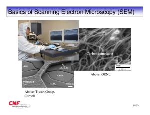
of the actual platform to use for developing remote control mainly depend on “non technical” conditions, as the availability of the instrument at lab or, starting with the acquisition of a new machine, its cost, completeness, suitability for different kind of users, and so on. Not the least, for the specific application, it is crucial the availability of programming libraries and the possibility to have, by the Manufacturer, the access to the proprietary codes of the software. The chosen instrument is a Quanta ESEM 200, made by FEI. It is an Environmental Scanning Electron Microscope (ESEM) that is a SEM able to introduce some partial pressure (air, water vapour or other gases) in the specimen chamber preserving the SEM operation. The instrument belongs to the latest evolution of the Scanning Electron Microscopy, that brooks the constraint of observing dry, conductive specimens, which heavily affect the direct observation, i.e., of biological specimens. The key point is that the residual gas around the specimen from one side neutralizes the beam-induced charging effects on dielectric specimens, and on the other allows the observation even of wet specimens, reaching the fascinating limit of observing water droplets by an electron beam. Anyway, the kernel of the operation is the same as for a standard SEM, and, for the sake of generality, the project focused on standard high-vacuum operation of the Quanta platform. The tele-microscopy project is started together with a bigger project that has regarded the realization of a “Microscopy and Nano - Analysis Laboratory”. Several

- 16 -

Chapter 2

The Scanning Electron Microscope

instruments had been acquired for this project, including the scanning electron microscope, and it has been decided to use it as the test bed for our remote control studies. Figure 2 shows the Quanta instrument. In the picture there is the scanning electron microscope and two computers to control it, the microscope controller PC, which operates directly on the instrument, and the support PC. The electron column containing the beam source, the specimen chamber, and the block with the pumps to create the high vacuum into the chamber have been highlighted to be easily identifiable. The Manufacturer introduces his product saying that [1]: “The Quanta ESEM 200 is a versatile high performance, low-vacuum scanning electron microscope with a tungsten electron source, with three imaging modes (high vacuum, low vacuum and ESEM) to accommodate the widest range of samples of any SEM system. The key features are: •

Seamless "point and click" transition between imaging modes;

•

Superior low vacuum, low kV imaging;

•

Simultaneous secondary electron (SE) and back-scattered electron (BSE) imaging in low vacuum mode;

•

Allows for in-situ dynamic experiments;

•

True surface (SE) imaging in all vacuum modes and voltages;

•

Easy-to-use, four quadrant/single quadrant user interface.”

- 17 -

Chapter 2

The Scanning Electron Microscope

Electron Column Specimen Chamber

Vacuum System

Fig. 2 The Quanta ESEM 200.

Fig. 3 The architecture of the Quanta local network [2].

- 18 -

Chapter 2

The Scanning Electron Microscope

The architecture of the machine aims to allow any microscopist to perform his analyses, storing and processing his images, possibly executing other software applications if required, but preserving the instrument from possible operation conflicts. To this purpose, a local area network (LAN) is made of two computers, one, the “Microscope Controller”, where the operating Quanta software is installed, and the other the “Support PC” dedicated to the operator’s utilities (see figure 3). 2.5

THE MICROSCOPE SOFTWARE On a practical ground, and beyond the commercial celebrations, the instrument is

indeed an excellent SEM and, at least under the technical point of view, an ideal platform for the proposed experimentation. The software interface is friendly and immediate; the commands are distributed following their function and their relevance. Figure 4 shows a snapshot of it. The four quads represent the image taken from different sources into the specimen chamber. The upper image on the left represents the image acquired from the secondary electrons detector; the upper image on the right side comes from the backscattered electrons detector. Downside, there are on the left a combination of the first two images, and on the right a lateral view of the inside specimen chamber taken by an internal camera, used to check the mechanical movements of the specimen, in order to avoid collisions and damages. The distribution of the images along the four quadrants may be set in many different ways, enabling other detectors, when available, or switching to a single wide frame. It is interesting to observe as really different emissions give different responses: the upper images are, in the screen, live pictures simultaneously updated as the beam scans the specimen surface, and refer to exactly the same area. On the right side of the image area of the user interface there are the commands to control the microscope parameters. The commands are organized in five pages, and grouped on the base of the managed parameters, even if the most important commands are present into each page.

- 19 -

Chapter 2

The Scanning Electron Microscope

The five pages

Fig. 4 The Quanta user interface.

The pages are named: Startup page Work page Option page Adjustment page Temperature page The other main parts of the user interface are: the “Menu bar”, and the “Tool bar”, whose buttons are located on the upper side of the frame. A detailed study of the characteristics of the instrument and the operations available with the Quanta software has been carried out, in order to define which characteristics and functions to include into the remote application, and which not, for the sake of instrument safety. This has been accomplished by page by page analysis, as reported in the following sections [2].

- 20 -

Chapter 2

The Scanning Electron Microscope

2.5.1 The Startup page The first page, named “Startup page” contains the commands used for changing the microscope parameters, for setting the work mode, for choosing the detector, and for verifying the microscope status during the analysis. The name used to identify these commands is: Vacuum, Mode, Electron Column, Source Control, Detector and Status. Table 1 gives a detailed description of the Startup page functions. Table 1 A detailed description of the Startup page. This frame allows the user to ventilate and pump the system, and to choose the working mode (High Vacuum is the default mode). If the Low Vacuum mode or the ESEM mode is selected, it is possible to adjust the pressure value into the specimen chamber using the scroll bar. Moreover, it is possible to choose the gas. Selecting the Pump button it starts the pump down of the specimen chamber. When the chamber is evacuated, the system allows switching on the high tension. Selecting the Vent button, the pump down process is stopped, and the specimen chamber is ventilated. Before to do this, the high tension has to be switched off. This frame regulates the electron beam parameters. The HV button is used to switch on/off the filament current; the High Voltage scroll bar allows to set the accelerating voltage of the electron beam from 0 to 30 KeV; the Spot Size scroll bar allows setting the beam size from 1 to 10.

The frame “Detectors” contains the scroll bar for adjusting the contrast and brightness values to optimize the displayed image. The minimum value is 1 and the maximum is 100 for both the parameters.

- 21 -

Chapter 2

The Scanning Electron Microscope

In this frame there are all the commands to saturate the filament after its substitution. After finding the new saturation condition, the voltage of the filament may be limited for the filament security. After the saturation, with the command Cross Over and Source Tilt it is possible to set the effective angle of illumination of the beam coming from the gun area of the electron column. The last section of the frame has a timer to monitor the filament life. When a new filament is placed, the timer starts to count the hours when the filament is switched on. Reset Timer is the button for resetting the timer value.

The frame Status shows the value of some parameters during the microscope working process, to monitor the state of the instrument. The parameters shown are: the Vacuum state of the specimen chamber, the high voltage value, the pressure value of the specimen chamber, the filament current value, and the emission current of the filament.

2.5.2 The Work page The second page is the “Work page”, and is different from the first because instead of the Electron Column commands, has the Stage Location commands, which are the commands to move the stage, and then the specimen. The following table shows in detail these commands.

- 22 -

Chapter 2

The Scanning Electron Microscope

Table 2 A detailed description of the Work page. This frame allows to change the coordinate of the stage, and then to move the specimen. In this page it is possible to move the specimen changing the position of the red dot that represents the specimen on the stage. The other signs presents are the stored positions. Using the button “Open”, “Save” and “Clear” it is possible to store, recall and then clear some specimen positions, in order to easy find again particular zones of the specimen.

This page allows the same functions of the previews; the difference is that to move the stage it is necessary to write the new coordinate values into the texts boxes.

2.5.3 The Option page The “Option page” is the third; it contains the commands to enhance the image displayed into the selected quadrant.

- 23 -

Chapter 2

The Scanning Electron Microscope

This frame, shown in table 3, replaces the Stage frame of the Work page. Table 3 A detailed description of the Option page. In this frame it is possible to set the magnification value and to correct the stigmatism value via the 2D box (X and Y coordinates).

The digital brightness and digital contrast correction may be used to correct the contrast and the brightness of an image already stored using a Gamma function. The “Reset” button brings the Gamma function back to default.

2.5.4 The Adjustment page The fourth page is dedicated to the beam alignment. Table 4 shows these commands; this page contains also the Status frame present in the Start-up page and shown in table 1.

- 24 -

Chapter 2

The Scanning Electron Microscope

Table 4 A detailed description of the Adjustment page. These commands are used to align the column and determine fine tuning for the electromagnetic system. As shown, various adjustments are available.

2.5.5 The Temperature page The last page has the temperature control. These commands are used with a particular stage that allows carrying out experiments at high temperature directly into the specimen chamber, to observe live the effect of temperature on the specimen. In table 5 these commands are shown. The other commands present in this page are present in the “Startup page” too, and are: the Vacuum frame, the Electro Column frame, the Detectors frame and the Status frame.

- 25 -

Chapter 2

The Scanning Electron Microscope

Table 5 A detailed description of the Temperature page. This frame switches between the Stage and the Peltier Cooling Stage two buttons at the top of the frame. These functions are used just particular functioning mode of the ESEM 200.

Heating via the during Quanta

2.5.6 The Menu bar The menu bar contains the classic menu bar commands, like “File”, “Window”, and “Help”, and other particular commands that are used to preset the following microscope parameters: magnification, accelerating voltage and spot size, scan functions and detector functions. Figure 5 shows the Menu bar, while table 6 explains its functions.

Fig. 5 The Menu bar. Table 6 A detailed description of each function of the Menu bar.

Administrative file functions. Choice of magnification presets. Choice of accelerating voltage and spot size presets. Associated scan functions.

- 26 -

Chapter 2

The Scanning Electron Microscope

List of detectors and control functions. Associated scan functions. Image auto functions and useful items. The image display functions. About Quanta UI and On-line help.

2.5.7 The Tool bar Finally, there is the tool bar at the top that contains some new commands, like the Auto Focus function, or the Auto Contrast and Brightness function. Some other commands present also into the menu bar are available; this is for giving a faster access to those commands. Figure 6 shows the tool bar, while table 7 gives a description of each command.

Fig. 6 The Tool bar.

Table 7 A detailed description of each function of the Tool bar.

Auto functions: these functions allow the auto contrast and brightness and the auto focus regulation. These functions give some more useful tools to adjust the contrast and brightness values, and the astigmatism correction. These commands concern the Magnification correction and the Z axis to Free Working Distance correction. These functions allow changing the scan velocity. This section contains the possible value of the pixel resolution of images displayed or recorded. These three functions are: the Beam Blanker, which allows to deflect the beam off axis and protect the specimen; the Snapshot to acquire the images; the Pause to stop the beam scan on the specimen. When the scan is paused, a symbol of pause is showed onto the image quad. These three symbols represent the possible filter functions applicable to the scanned image. This command allows sharing the desktop with another PC using the VNC program.

- 27 -

Chapter 2

The Scanning Electron Microscope

Selecting this button the recording of a video from the three quads with the specimen images will start at the same moment. Clicking this button, the On-line help window will be opened.

2.6

WORKING WITH A QUANTA MICROSCOPE As described above, a Quanta microscope has several functions. Some of those

are standard functions of a scanning electron microscope; others are related to the particular model of instrument (Quanta ESEM 200). This research work aims to give the origin to the remote microscopy developing a remote application independent from the microscope used as test bed instrument. With regard this aspect, it is interesting to see how the normal procedures to carry out an analysis with a SEM are performed with a Quanta microscope. The first operation is to ventilate the chamber to insert in the specimen. To do this, it is sufficient push the button “Vent” contained in the “Startup page”; a dialogue box will ask “Really vent the chamber?”; choosing “Yes”, the pumps are automatically stopped, and the valve to introduce the gas into the chamber is opened. This dialogue box is a secure system, which should avoid ventilating the chamber accidentally. During the ventilation phase, in the box “Status” included into each page, the Vacuum Status is “Venting”, the quad is not green but yellow and the value of pressure increases rapidly. When the chamber is totally ventilated, the Vacuum Status shows “Vented”, and the quad is red. Now it is possible to open the chamber pushing the frontal side, and to place the specimen on the stage, and close again the chamber. The next phase is to activate the vacuum pumps pressing the button “Pump” on the “Startup page”. Then, the pumps will activated automatically, and the Vacuum Status will be “Pumping”, while the pressure value on the Status box will decrease rapidly. When the vacuum pressure value is reached, the Vacuum Status will be “Vacuum”, and the button to turn on/off the High Voltage will be enabled. At this point it is possible to turn on the high voltage pressing the button “HV” on the user interface and the first images of the specimen will be displayed on the monitor of the microscope controller computer. Also in this case, the image usually is not well focused and properly balanced.

- 28 -

Chapter 2

The Scanning Electron Microscope

To focus the image it is necessary to calibrate the height of the specimen (that is the z axis) with the electron beam focused; before to perform this operation, the automatic movement of the stage along the z axis is forbidden, while the movement is allowed along the other axes. The “Stage Location” box into the “Work page” shows the value of each coordinate; then, reading here the z coordinate value, it is possible to focus the electron beam at this point. To complete the calibration operation, it is necessary to push the button for the “Z axis to Free Working Distance Correction” included into the Tool bar. Now the z axis and the focused electron beam are calibrated, and the focusing operation of the image will be performed just operating on the lenses; the automatic movement along the z axis is enabled too. The Quanta software allows focusing the image also pressing the right mouse button and moving the mouse to the left or right on the image. This is a specific Quanta operation that simplifies a lot the focusing operation. The other operations to optimize the quality image are performed using the buttons in the user interface. To set the contrast and brightness values, the scroll bars in the “Detectors” box have to be used. The high voltage value and the spot size values may be set from the “Electron Column” box. The magnification can be changed into three modes: clicking the “Magnification” menu in the Menu bar and choosing a value, scrolling the scroll bar in the “Option page”, or pressing the “+” and “-” keys on the keyboard. Also this last way is a specific Quanta solution. The system of images acquisition consists in a digital device which acquire the images as if it is a digital photo camera. Before to acquire the image it is possible to set the pixel resolution, choosing the size of the acquired image, and to set the scan speed; slower is the scan speed, higher will be the resolution of acquired image. The buttons to set the scan speed are into the Tool bar, and are the “+” and the “-” near to the rabbit (faster) and to the turtle (slower). To do this there is also another procedure, finer because it allows setting the time to perform a line scan and a frame scan. Also clicking the Scan menu in the Menu bar it is possible to change the scan speed. The commands to set the pixel resolution are included in the Tool bar too. After the setting of these parameters, clicking the “Snapshot” button on the Tool bar it is possible to acquire the image. The images are stored in the Support computer; this is a secure system specific of the Quanta instrument. Another particular aspect of the Quanta interface is that each of

- 29 -

Chapter 2

The Scanning Electron Microscope

the most used commands can be activated with different modes, some faster, and some finer (more precise).

- 30 -

Chapter 2

The Scanning Electron Microscope

REFERENCES [1] http://www.feicompany.com. [2] The standard user manual of the FEI Quanta microscope.

- 31 -

CHAPTER 3 THE DEVELOPMENT OF THE PROJECT

The focus of this chapter is to describe all the phases of the remote microscopy project from the starting plan to the ultimate version of the remote application. This will include the dramatic program change that forced to abort the first idea because of technical difficulties unknown even to the Manufacturer.

3.1 THE REMOTE ELECTRON MICROSCOPY The remote electron microscopy is not a recent idea, and, along the years, numerous solutions have been attempted to realize it. The relevant difference between them is the concept of remote microscopy that they represent. In fact, the remote microscopy could be achieved in more than one way, depending on the purpose. If the function is to satisfy some training requests, the remote microscope is just a demonstrative application as proposed in the Virtual SEM Project [1], by the Imaging Technology Group [2], Beckman Institute, University of Illinois, USA. The remote application developed by this laboratory is a web based application and the test bed instrument is a Philips XL-30 ESEM-FEG. The remote application is developed for educational reasons, and the available operations for the remote control are: contrast and brightness setting, image focusing, magnification regulation, status bar, and more an interactive chat system between the remote operator and the local operator. The limits of this application are the restricted access to the instrument, justified maybe by

Chapter 3

The development of the project

the educational goal, but that inhibits the possible applications of it by several different users. Another example developed for educational reasons is located at the University of Michigan (John F. Mansfield, North Campus Electron Microbeam Analysis Lab, University of Michigan, USA [3]). In this case, to achieve the remote control, an already existing tool has been modified. The remote access to the microscope is performed using a modified version of the Virtual Network Computing (VNC®) software, developed to remote control the computers through the network. In this case the local operator gives the control to the desktop to the remote operator. The cons of this solution are the low quality of the image transmitted, and the not real time interaction between the remote operation and the instrument. A similar solution has been applied into another laboratory (Centro Grandi Strumenti, University of Modena and Reggio Emilia, Italy [4]). Here, the tool used has been NetMeeting®, but only some microscope commands are available, like magnification and brightness. Like the previous example, the interactivity between instrument and remote operator, and the very bad image quality are the weak spots of this solution. To summarize: very local networking and the low quality and high delay of the standard video streams along the net are the main reason for achieving at most a demonstrative level, but not real remote operative conditions. The concept of remote microscope used in this project is different; the remote control is not an existing software tool adapted to the microscope, but is a new application developed for this instrument, and that gives the possibility to use it as if the operator was in front of it [5]. The complexity of this project is important and relevant, and its development has been long and challenging, but the work is justified from the importance of the instrument into each laboratory, both those of the Universities and those of the private societies. The application will work at the same mode for all possible remote users: the difference will be in the operations allowed to them. An expert user will be enabled to perform a complete SEM session; a student will have only some commands allowed, like brightness, contrast, magnification, but he will not manage, for example, the high tension or the pressure chamber; a customer not microscopist, will be just a spectator. This project is started from the feasibility study, because it was necessary to develop a software application. After this, the work has continued determining the characteristics and the features that the application should satisfy, and after the

- 33 -

Chapter 3

The development of the project

possible solutions have been identified. The last step has been the choice of the kind of solution, and its implementation. 3.2

THE FEASIBILITY STUDY As illustrated in the previous chapter, the Quanta ESEM 200 has a lot of technical

features that make it an instrument unique and distinctive. Anyway for this research work the fundamental characteristic is a peculiarity of its architecture: the internal LAN that connects the Support PC and the Microscope Controller PC. Accessing that LAN will open the door to the remote control. This has been guaranteed from the Manufacturer, which supplied a Dynamic Link Library (DLL) developed exactly to interface an external application with the microscope software. This Library consists of a series of Component Object Model (COM). Together with this, the Manufacturer has given another application, a Distributed Component Object Model (DCOM) client. This object is an extension of the Component Object Model (COM) that allows COM components to communicate across network boundaries. This application, installed on a computer connected with the microscope internal network, allows an application developed with the library to interface itself with the microscope. Figure 1 shows the internal network of the Quanta instrument.

Fig.1 The block diagram of the instrument connections.

- 34 -

Chapter 3

The development of the project

The following point has been the test of these libraries, named XTLibInterface®. These libraries consist of a series of COM object directly instantiable and their COM interface retrievable by a client application through COM. The testing phase has concerned the main libraries function, to verify the working system, and the code implementation. The programming languages supported are Visual Basic e C++; the testing tools have been developed using the Visual Basic language. 3.3

DEFINITION OF SPECIFICATIONS In this phase, the main attention was paid to establish what the final application

should do. First of all, the following features have been fixed: 1.

The user interface of the remote application should be friendly for a standard microscopist: it should enable a remote operator to use the microscope as if he was in front of it.

2.

All the microscope commands necessary to perform an analysis with it have to be available for the remote operator. These have been identified in: high voltage ON/OFF, to set the high voltage value, the chamber pressure value, setting the brightness and the contrast, the spot size value, the magnification value, to select scan speed, to focus the image, to move the specimen stage, and to rotate the electron beam. All these functions are available with the XTLibInterface® libraries.

3.

The remote and the local operator should communicate directly, through a chat, for instance. A system as a chat is useful to change information between the operators that are attending the analysis, and also the possibility to work together on the same image, for example, it should be useful. In order to satisfy this last point, it could be added a digital blackboard to the chat.

4.

To carry out a microscopic analysis, it is necessary to look at the specimen; then, it will be necessary to enable the remote operator to see the specimen sending the same video observed by the local operator. The first solution consists to take the video card output; to be sent on the

- 35 -

Chapter 3

The development of the project

network, the video has to be elaborated and streamed with appropriate coding standard. 5.

The last aspect considered is the application security. The scanning electron microscope is a very expensive instrument, and although it has several systems of protection against not allowed operations, it is necessary to provide also the remote application with a system security. This system should monitor the access to the microscope, allows the enabled remote operators, and blocks the not allowed clients which try to enter to the microscope.

3.4

DESIGN The purpose of this phase was to identify the solution after the features

description. Two solutions able to satisfy all the characteristics defined have been found. The first is a server/client application consisting of the development of two different applications, a server application and a client application, able to communicate between them. The second solution is a web based application consisting of a particular web site that allows the access to the microscope. A detailed study of pros and cons for each solution has been carried out. 3.4.1 The Server/client approach This approach consists of the implementation of two different applications, a server application and a client application able to communicate between them using the TCP/IP protocol. The server application must be installed into a third computer near the microscope, and connected to the microscope controller PC through the Support Network, (figure 1). The client application will be installed into the remote operator’s computer, and will connect to the server through the customer LAN. The first step has been the classification of pro and cons of this solution, just to test the convenience and the efficiency. The pro identified are: 1.

Interactivity

- 36 -

Chapter 3

The development of the project

2.

Friendly interface

3.

Reliability

4.

Security.

The only negative aspect is the portability. The interactivity and the friendly interface are due to the programming language chosen. The Visual Basic language, in fact, is specified for developing applications that need a user interface, and then it is simple to implement user interfaces easy to use. The relevance of this possibility is that a friendly interface enables the remote user to understand immediately the application use, without reading long manual or complex instructions, facilitating the interactivity between operator and microscope. Developing two applications, a server and a client, able connecting between them, it is easier to control the reliability and security of the application. First of all, only the allowed users can access to the instrument, through a login with user ID and password assigned by the microscope administrator. Second, an encrypted communication to send the information will be used, in order to mask the sender and the receiver. The portability is seen as a disadvantage, because the applications will be developed for the Windows® Operating System, the same Operating System of the PC microscope controller. Then, to use the application with another Operating System, another dedicated application has to be developed. The video elaborating system is realized using a video encoder together with the server application, which takes the video card output and a video player together with the client application, which is able to play the video sent by the encoder. A more detailed explanation of this aspect will be given in the next chapter. 3.4.2 The web based approach This alternative solution aims to achieve a web site using the Active Server Page (ASP) technology in conjunction with the HTML language. The reason of these choices is that the ASP technology supports the Visual Basic Script language that is a programming language similar to the Visual Basic language, but easier; the HTML language will be used to develop the user interface.

- 37 -

Chapter 3

The development of the project

The project establishes that the web server is the same computer that should support the server application of the first solution. Then, in this computer an Internet Information Service (IIS) of Windows will be activated. The access to the web site allows the access to the microscope; the web site access will controlled giving a user name and a password to the remote operation, and using the HTTPS protocol to transfer the microscope web pages. This protocol is the protocol HTTP (Hyper Test Transfer Protocol) used in conjunction with the Secure Socket Layer protocol (SSL). The web pages will contain the microscope commands, and there will be a frame where play the video stream sent by the encoder. In fact, the video elaboration principle is the same as the first solution; the difference is that the player is embedded in the web page. In the other case it was a separate application. The positive aspects of this way are the available friendly interface, the reliability, the security and the portability. That negative is the interactivity. Then, the characteristics are a little bit different from those of the server/client application. In fact, a web site is accessible from every internet user, independently from the Operating System used. Vice versa, the interactivity available with the ASP technology and the VBScript language is limited from the language and the technology itself. Considering the positive and negative aspects of both selected solutions, the web based solution has been preferred. The decision has been made especially in view of its portability, more significant than its low interactivity. 3.5

THE IMPLEMENTATION OF THE WEB APPLICATION The web application development has been divided into two parts: the

implementation of the VBScript code for the microscope commands and the HTML code for the user interface, and the development of the video coding system. The first part is started organizing the web pages structure. The home page is the access page; here there is the login by user name and password, and then the loading of the page with microscope commands. Figure 2 shows this page.

- 38 -

Chapter 3

The development of the project

Fig. 2 The home page of web based application.

After some tests carried out in order to find the best implementation of the commands for managing these independently, it was decided to use the HTML frameset. The microscope commands have been grouped on the base of their function, and a frame for each group has been projected. This work has been carried out developing the frames separately, and testing it. The implemented frames are: “Status”: here it is possible to read the pressure value, the specimen chamber state, and the form functioning of the microscope. The test is positive. “High Voltage”: this frame gives the high voltage control; here it should be possible to read the voltage value, to turn on/off the beam voltage, and to set the value. The result of testing this frame is that it is possible to read the value, but not to set it or turn on/off the voltage. “Magnification”: in this frame the commands to read and set the magnification value are located. Developing it, some errors have been found. In fact, when it has been loaded for testing, a signal error has been given from the system. “Contrast and Brightness”: in this frame there are the commands to read and set the contrast and the brightness value. The value is correctly changed, but to see the new value it is necessary to reload the frame.

- 39 -

Chapter 3

The development of the project

“Image”: this frame is dedicated to display the images of the microscope; testing the frame, there is the same error as the magnification frame when it is loaded. At this point, before to continue with the framesets implementation, considering the number of errors of the already done implementations, a series of tests was programmed to debug them. 3.5.1 The debugging phase The debugging phase has been carried out first frameset by frameset. Then the framesets were integrated into the web site, and tested again one at a time. The web site test was performed into two different moments: before it was carried out trying the connection to the site from the same web server computer; in the second moment, the connection to the web site was tried from another computer, different from the server web, and different from the microscope controller. The results were that the framesets that worked independently and in the local server worked also in remote server; the framesets that did not worked independently, did not worked also integrated into the web site. To resolve this problem, different implementation solutions have been tried, without achieve relevant results. The reason of those problems is that not all the functions of the XTLibInterface® are compatible with VBScript, and then it was normal that some of these gave error when implemented. The root cause was clearly inside of the Manufacturer’s proprietary code, and then the Manufacturer was asked for assistance. They suggested to use only Visual Basic programming language, because it was the first edition of the XTLibInterface® and they tested successfully only the Visual Basic language. The other languages, like C++, or also VBScript were not tested, and then not reliable. At this time, the entire web based project was aborted, and the research work was focused on the other solution, the server/client application. 3.6

THE IMPLEMENTATION OF THE SERVER/CLIENT APPLICATION The server/client applications are particular kind of applications, which can be

implemented following two predefined architectures: a two level architecture and a three level architecture. The number of levels depends on the number of the breaks

- 40 -

Chapter 3

The development of the project

between the data origin and the client application. In this case there are three levels because the server application, to satisfy the client requests, has to forward these requests to the microscope. Then, the server application is a client for the microscope, as shown in figure 3.

REQUEST

CLIENT

REQUEST

MICROSCOPE

SERVER

ANSWER

ANSWER

Fig.3 The data flows from the client to the microscope

To build two applications able to communicate, a particular software object has to be used: the socket. Using Visual Basic as the programming language, the object used has been Winsock. The socket is a software object that connects an application to a network protocol. Then, using it both for the client and the server application, these will be able to connect to the network and the client will connect itself to the server using the server IP address. The server is then connected to the microscope controller computer through the DCOM client, and then can forward the client requests to control the instrument. Also this implementing work has been divided into two parts: the implementation of server/client applications to control the microscope, and the implementation of the video application. The last will be explained in detail in the third chapter. To realize the first part, the work started from the code written to test the XTLibInterface®. The already developed functions have been integrated into a unique form. At the same time, the not yet added functions have been first tested and then integrated. The main attention during this work has been paid on the user interface configuration. In fact, the remote microscopes are not a commercial product, but there are few prototypes into some research laboratories. One of the goals of this work is to implement a standard for the remote microscope. Then, the user interface developed

- 41 -

Chapter 3

The development of the project

should be not related to the instrument used for the experiment, but standard and useful at the same time, so that an expert microscopist can use it immediately, while a not expert user can learn easily the instrument working process. For these reasons the most important is the user interface of the client application; the server application, in fact, will be installed onto a PC sited in the same room as the microscope, then nobody will use it to control the microscope, but just to control the remote connection. The only active commands are those related to the connection with the client application (table 1). All the other commands are not enabled, while into the text boxes included in the user interface the server writes the values received form the microscope controller application. Figure 4 sketches this user interface. Table 1 The commands related to the connection included in the server user interface When the client requests the connection to the server, to allow the connection the server has to push on the button “Connect”, while the button “Disconnect” interrupts the connection. The button “Run Microscope” can be used to connect the server application to the microscope without any client application connected to it. The label “Disconnected” reports the connection state. This is the chat frame: the server writes the message into the box below, and pushes “Send” to send them to the client. In the upper test box all sent messages are displayed.

- 42 -

Chapter 3

The development of the project

Fig. 4 The server application user interface

The other characteristics considered during the development of the user interface have been: the functionality, the layout, and the connection security. In fact, it is important, for example, to keep the interrelated commands close each other, as the high voltage turn on/off and the high voltage setting. At the same time, it is important to have commands simple to use and giving a real time reaction (as example, a scroll bar to change the contrast and brightness value instead of a text box where put the value). The security is decisive to preserve the microscope from incorrect use and then possible damages. The server/client application realized until now satisfies almost these features. In fact, it is simple to use, and it is not related to the original microscope interface. As it is possible to see from figure 5, the commands have been grouped on the base of their function. Moreover, relating the user interface developed with the Quanta user interface it is immediately to note that are not corresponding. Looking the picture, it is possible to distinguee the different frame created to group the analogous commands.

- 43 -

Chapter 3

The development of the project

Fig. 5 User interface developed for the client application.

The following table explains each frame in detail.

Table 2 The microscope commands included in the client user interface grouped in frames on the base of their function. The frame “Electron Column” contains the commands to turn on/off the filament voltage, to set its value, and to set the spot size value.

The frame “Focus” contains the commands to focus the image using the free working distance.

- 44 -

Chapter 3

The development of the project

The frame “Detectors” contains the commands to set the contrast and the brightness values.

This frame gives the possibility to know which kind of detector is installed, and which detector is already active.

The frame “Rotation” gives the possibility to rotate the image changing the scan direction of the electron beam. The frame “Dwell Time” allows the user to change the scan speed of the electron beam.

The frame “Magnification” contains the command to change the magnification selecting directly the size scan area onto the specimen. Increasing the area selected, the magnification decreases. The frame “Stage” allows the user to move the stage, then to move the specimen mechanically. The values of the axes are changed independently. The T value is the value of the tilt rotation; this value is changed manually, then it is only possible to read it.

The frame “Status” contains a report about the working conditions of the instrument. The data reported are: the High Voltage, the Pressure chamber, the microscope working mode, and the chamber pressure state.

The frame “Vacuum” gives the possibility to change the pressure value while the microscope is working in the Low Vacuum or ESEM mode.

- 45 -

Chapter 3

The development of the project

The “Stigmator” frame allows the astigmatism correction of the images, following the axis of a two dimensional Cartesian system.

The “Channels” frame allows making on pause state the image onto the screen; the CCD channel is the image of the specimen chamber given from the digital camera; the other channel is the channel selected from the operator, than it could be the Secondary Electrons image, the Backscattered Electrons image, or someone else.

The above explained frames are all related to the use of microscope. The other frames located in the user interface contain specific commands to use the client application in conjunction with the server application. Table 3 explains them. The connection is based on the TCP/IP protocol: the client searches the server by its IP address. The transmission occurs by two separated channels: a channel from the client to the server, and a channel from the server to the client, in order to decrease the probability to loose some data. At the moment, the connection it is possible just for one client at a time, but it is possible to enlarge the authorization for more clients. In order to respect the security conditions, each client will connect to the server by a particular user name and password, and the server has to recognize it before to allow the connection. Table 3 The commands concerning the connection between the client application and the server application included in the client user interface. The “Server Connection” frame is the frame where there are the commands to connect the client application to the server application. In the text box, the client inserts the IP address of the server, and then clicks on the button to request the connection. When the connection is allowed, the button label becomes “Close” (the connection), and the other labels indicate the channels transmission state.

- 46 -

Chapter 3

The development of the project

The “Connection” frame is the frame to connect the client application to the microscope. Before to establish the connection, all the buttons are red; as first, the client clicks on the button “Connect”; the series number of the microscope will sent from the server and the Button “Run Microscope” is enabled; after, the remote operator clicks this button and the microscope commands of the client user interface will be enabled. These two buttons become then green, while the button to disconnect the client from the microscope is enabled and becomes yellow. The “Chat” frame gives the possibility to the remote and the local operator to communicate using the chat. The client writes its messages into the white text box, and then clicks “Send” to send the massages to the server. In the upper text box will be displayed all the messages written by the client and the server.

Besides the frames, in the user interface there are the menu bar; this is similar to that of the original Quanta software; the reason is that the functions present are typical functions for every scanning electron microscope. Then the reproduction of this menu bar does not represent a loss of standard characteristics for the remote application here developed. 3.6.1 The debugging phase The testing phase has been carried out after each modification of the software. In fact, the functionality of different microscope functions was already tested at the beginning of the research work; in this phase it was necessary to debug the Visual Basic code. Different errors have been found into the code, and have been removed following the debug indications. The testing phase has been very useful to realize a good user interface, and especially to establish a correct connection between server and client.

- 47 -

Chapter 3

3.7

The development of the project

WORKING WITH A REMOTE SCANNING ELECTRON MICROSCOPE In order to give a comparison between to use the microscope locally and

remotely, a sequence of the actions performed to carry out a remote analysis will follow. When the remote operator starts to work with the remote microscope, the first operations that he has to perform are related to the connection from the client application to the server application. He requires the connection to the server, and if the server allows it, he connects the client application to the microscope, and can start to use it. The starting operation of a microscope analysis is to introduce the specimen into the chamber. If the chamber is on the vacuum state, it is necessary to stop the vacuum pumps and to ventilate it. These operations are not performable on remote, then the local operator, always present in front of the microscope, has to do it. Obviously, he has also to introduce the specimen in the chamber and to start the vacuum pumps to evacuate the air from the chamber. When the chamber has reached the desired pressure, the remote operator may turn on the high voltage, and he can see the image of the specimen. The next operation, as described in the previous chapter, is the calibration of the z axis. This operation is not performable as a remote operation, then the local operator has to do it. After the calibration, the remote operator will be able to focus the image only focusing the electron beam. The other commands to improve the image quality are enabled since the beginning, and the remote operator can use it as if it is in front of the instrument. It is simple to note from this description that the use of the remote microscope is not so much different from the local use. The commands included into the user interface are standard commands, and each microscopist may use it without knowing the kind of the instrument. 3.8

COMMENTS The project, as described up to now, achieved the target of developing a

dedicated application for remote controlling a SEM. The important chapter of the video handling has yet to be presented. Anyway, it may be time to compare the

- 48 -

Chapter 3

The development of the project

achievements here reported with the examples reported at the beginning of the chapter. The first example (University of Illinois) is similar to the first solution here studied; it is a web based application, but its user interface includes only few commands, not sufficient to obtain exhaustive analyses and high quality images. The second example (University of Michigan) has a complete different approach, because it does not implement any user interface, but it sends the user interface proper of the instrument to the remote operator. This is different form the main goal of the reported research work: the standardization of the remote microscopy. Sending the proper interface of the instrument, the remote user will be locked up of learning the use of that particular microscope. The last example reported (University of Modena) differs into the approach; also in this case it uses an already existing tool (NetMeeting®), and no much commands are available for the remote control. Moreover, the image quality is very bad and the real time interactivity is not reached.

- 49 -

Chapter 3

The development of the project

REFERENCES [1] http://www.itg.uiuc.edu/technology/remote_microscopy. [2] http://www.itg.uiuc.edu. [3] http://emalwww.engin.umich.edu/people/jfmjfm/jfmjfm.html. [4] http://www.cigs.unimore.it. [5] F. Mighela, C. Perra, “Remote Control for Microscopy Applications”, submitted to Instrumentation and Measurement technology Conference, Sorrento, Italy, April 2006.

- 50 -

CHAPTER 4 THE VIDEO TRANSMISSION

Vision is the base of microscopy. In this chapter an insight on the creation and handling of the images in a SEM will be given, and then how these images are made available to the remote operator.

4.1 THE MICROSCOPE VIDEO Different from other remote applications where the eyes and the hands of the operator are moved off the operation field, and primarily ask for instrumental substitutes to emulate the human presence on site, the SEM interfaces even with the local operator by a video screen and a set of commands that are linked to the internal sensors and actuators by some software interface. The possibility to pipe the command set into a long distance net has been illustrated in the previous chapter, and the tests showed the capability to drive a SEM through a loop connection: a keyboard in front of the SEM screen was connected to the instrument via a server-client connection running on the general LAN of the University, or even on external public networks. The SEM reacted as under local commands, without errors or delays. In other words, the remote control was fully demonstrated, while the operator-microscope interaction was obtained by direct observation of the local, non remote, LCD screen.

Chapter 4

The video transmission

Now, a microscopist works looking at a “live” specimen, that may also be the most unanimated crystal, but continuously moves, enlarges, sharpens, lightens under the solicitation of the instrument controls. Then also a remote microscopist should look at the specimen in the same way. The simple idea is to send to the remote operator exactly the same images observed by the local operator, without any data loss, and without any delay. This simple statement makes the real challenge of the whole project, and for this reason a significant part of the research work has been dedicated to it. The crucial point is that a video stream needs a compromise between bandwidth and data compression or even data loss. Moreover, any video encoding introduces some time delay. Both things keep the remote user actually “far” from the instrument. In order to find a solution, the microscope video architecture has been studied. 4.2 THE MICROSCOPE VIDEO ARCHITECTURE The image of a Scanning Electron Microscope is created measuring the intensity of the current of secondary electrons or backscattered electrons emitted from the specimen under the stimulus of the electron beam. Several different detectors have been developed for the electron microscopes, and the most celebrated one in Scanning Electron Microscopy, the Everhart-Thornley scintillator-photomultiplier, is described in Appendix B. In any case, the detector outputs an electric signal proportional to the collected electron intensity: as the beam scans the specimen surface, the signal changes according to the variation of the electron emission. In the last generation instruments, the analog response of the detector is sent to an analog to digital converter, whose output is used to write the video memory, according with the scanning sequence of the image field. The signal thus generated is processed by a Variable Data Rate Video (VDRV) processor. This kind of processors is able to vary the amount of data processed per frame to match image quality and transmission bandwidth requirements. The output of this processor is the input of the frame grabber card. The role of the frame grabber is to decouple the video input and output formats, allowing to read the frame buffer according any supported video standard, although its live update usually proceeds at highly non-standard rate (number of pixels per line and per frame, pixel, line and frame times, etc.) from the VDRV processor. The frame grabber installed in the

- 52 -

Chapter 4

The video transmission

microscope used in this project has four inputs, and each input may be independently used. In the QUANTA platform, three of these usually have as input the output of the multi-channel VDRV processor. In this way, different live images from different detectors may be simultaneously displayed. The fourth input is usually the video output of the digital camera that looks at the specimen chamber from inside, as shown in the images in the previous chapters. The frame grabber video output is then sent through the PCI-bus to the video card and it will be overlaid onto the windows background. The LCD monitor of the microscope controller is connected to the output of the video card. The following picture sketches a LCD monitor view; here it is possible to see the four quads that reproduce the four video output of the frame grabber (figure 1).

FIRST QUAD:

SECOND QUAD:

SECONDARY ELECTRONS IMAGE

BACKSCATTERED ELECTRONS IMAGE

THIRD QUAD: COMPOSITION OF FIRST QUAD AND SECOND QUAD IMAGES

FOURTH QUAD: INTERNAL DIGITAL CAMERA VIEW

Fig. 1 The visualization of the four video sources elaborated by the frame grabber.

- 53 -

Chapter 4

The video transmission

4.3 THE VIDEO ARCHITECTURE DEVELOPMENT Starting from this architecture, the planning of the architecture to perform the video streaming is started. This phase has divided into more parts: first the study of the system properties, then the planning of the architecture solution, and last the choice of the technology. 4.3.1 The system properties First of all the requirements for the video transmission have to be identified; this should be a real time and full resolution transmission. The real time is justified for the necessity of a microscopist to see immediately the alteration made on the image, like the variation of the contrast, or the variation of the magnification, while the full resolution is necessary considering the size of the objects analyzed. The factor that has the main influence on the availability of these properties is the relation between the bandwidth available and the bandwidth required for the transmission. The currently available bandwidth has been estimated with several tests at the SEM laboratory; the result was that the network average bandwidth available for the transmission is about 10 Mbps. This encouraged to proceed, because the typical byte rate in a SEM (that is simply the pixel dwell time) is 1 MBps. A more detailed analysis showed that the video microscope size is not always the same, because it is possible to choose the resolution and the pixel dwell time, that ultimately define the frame rate. The worst case, considering a dwell time of 0.1μs (the faster available), is with a resolution of 512x442 pixels, while the best case is a resolution of 3584x3094 pixels. This means that the video microscope has to be manipulated to be sent on the network; in particular it has to be compressed. Table 1 shows the compression ratio calculated for every resolution value available at the microscope, considering a frame rate value equal to 10 frames per seconds. Looking at the table, the worst case has a very low signal-to-noise ratio, and the images are not significant and comprehensible, while the best case does not allow useful analysis (the refresh time is too long). These cases are extreme situations; in the table there are middle resolution values, with a good compression ratio. Normally,

- 54 -

Chapter 4

The video transmission

the resolution used is 1024x884 pixels, with a frame rate of 10 frames per seconds, because it reaches a good compromise between noise reduction and scan speed.

Table 1. Trade-off between video resolution and compression ratio.

Microscope

Frame rate

Compression

resolution (pixel)

(frame per second)

Ratio

512 x 442

10

1:1,81

1024 x 884

10

1:7,24

2048 x 1768

10

1:29

3584 x 3094

10

1:88

4.3.2 The video architecture design Together with the video architecture design, also the technology has been decided. The video architecture designed is a video streaming architecture. The technology chosen is based on the H.264/AVC compression standard. Figure 2 shows a block diagram of it.

MODIFIED H.264

STREAM

VIDEO CLIENT (STANDARD CLIENT H.264)

FRAME ANALYSIS

FRAME GRABBER

DECODER

OUTPUT

LOCAL VIDEO

Fig. 2 The block diagram of the architecture designed for the video application.

In order to give a more detailed explanation, a description of each block follows.

- 55 -

Chapter 4

The video transmission

Frame grabber: this block is the frame grabber card. In the used instrument it is a Viper-Quad card, made by the Dalsa Coreco Society. The Viper-Quad is a single slot high speed video acquisition device for the PCI bus [1]. It features four independent acquisition channels each comprised of an 8-bit analog-to-digital converter, synchronization circuitry, anti-aliasing filter (optional), and input lookup tables. The four channels can acquire images from four non-genlocked monochrome cameras. Each channel also supports separate horizontal and vertical sync signals (input or output), a trigger input (optically isolated for protection from potentially hazardous voltages), a trigger output, exposure control output, and a strobe output. The features described permit each channel to acquire images from four completely independent cameras. The Viper-Quad installed in the Quanta microscope acquires the image taken with the electron detectors and converts it into a standard video format. Local video: this block represents the video card of the microscope controller computer, which receives from the PCI-bus the Viper-Quad output and overlays it with the window background. Frame analysis: this block takes the output of the frame grabber, and analyses it before to decode it with the H.264 encoder. Modified H.264: this block decodes the output of the frame grabber and compresses it on the base of the H.264 international standard. Stream: the stream block allows the transmission on the network of the coded video. Decoder: this block is at the end of the network transmission, on the remote client side, and decompresses the received video streamed. Video Client: is the application that allows the remote operator to see the video decode by the decoder. It is a video player, and it can be any video player H.264 compatible. The more interesting and delicate aspect of this architecture project is the video encoder; from it depends the satisfaction of the system properties above analysed. There are more then one way to achieve a suitable encoder; the first possibility is to choose a commercial encoder, and testing its performance on the system; the second is to realize a dedicated encoder. In the last case it will be possible to adapt the encoding architecture and, in particular, the encoder parameters, to the type of content and maximize the compression efficiency. Anyway, all these possible solutions have a common aspect: they will be based on the H.264/AVC compression standard.

- 56 -

Chapter 4

The video transmission

The reason is that at the moment this is the best compression standard available. Here a brief description of its main features is given, while a detailed description of the encoder planning follows. 4.3.3 The H.264/AVC video coding standard H.264/AVC is the latest international video coding standard [2]. It was jointly developed by the Video Coding Expert Group (VCEG) of the ITU-T and the Moving Picture Expert Group (MPEG) of ISO/IEC. It uses state-of-the-art coding tools and provides enhanced coding efficiency for a wide range of applications, including video telephony, video conferencing, TV, storage (DVD and/or hard disk based, especially high-definition DVD), streaming video, and many others. H.264/AVC was developed over a period about four years. The root of this standard lie in the ITU-T’s H.26L project initiated by the VCEG, which issue a Call for Proposals (CfP) in early 1998 and created a first draft design for its new standard in August of 1999. In 2001, when ISO/IEC’s MPEG had finished development of its most recent video coding standard, known as MPEG-4 Part 2, it issued a similar CfP to invite new contributions to further improve the coding efficiency beyond what was achieved on that project. VCEG chose to provide its draft design in response to MPEG’s CfP, and proposed joining forces to complete the work. Several other proposals were also submitted and were tested by MPEG as well. Therefore, to allow speed progress, ITUT and ISO/IEC agreed to join forces together to jointly develop the next generation of video coding standard. In order to satisfy the wide areas of applications considered by the two organizations, three basic features sets called profiles were established to address these application areas: the Baseline, Main, and Extended profiles. The Baseline profile was designed to minimize complexity and provide high robustness and flexibility for use over a broad range of network environments and conditions; the Main profile was designed with an emphasis on compression coding efficiency capability; and the Extended profile was designed to combine the robustness of the Baseline profile with a higher degree of coding efficiency and greater network robustness and to add enhanced modes useful for special “trick uses” for such applications as flexible video streaming. The new standard has been designed for technical solutions including at least the following application areas [3]:

- 57 -

Chapter 4

The video transmission

•

Broadcast over cable, satellite, Cable Modem, DSL, terrestrial, etc.

•

Interactive or serial storage on optical and magnetic devices, DVD, etc.

•

Conversational services over ISDN, Ethernet, LAN, DSL, wireless and mobile networks, modems, etc. or mixtures of these.

•

Video-on-demand or multimedia streaming services over ISDN, Cable Modem, DSL, LAN, wireless networks, etc.

•

Multimedia Messaging Service (MMS) over ISDN, DSL, Ethernet, LAN, wireless and mobile networks, etc.

Moreover, new applications may be deployed over existing and future networks. This raises the question about how to handle this variety of applications and networks. To address this need for flexibility and customizability, the H.264/AVC design covers a Video Coding Layer (VLC), which is designed to efficiently represent the video content, and a Network Abstraction Layer (NAL), which formats the VLC representation of the video and provides header information in a manner appropriate for conveyance by a variety of transport layers or storage media. See figure 3.

C O N T R O L D A T A

VIDEO CODING LAYER Codec Macroblock DATA PARTITIONING Codec Slice/Partition

NETWORK ABSTRACTION LAYER H.320

MP4FF

H.323/IP

MPEG-2

Fig. 3 Structure of H.264/AVC video encoder.

- 58 -

etc.

Chapter 4

The video transmission

4.3.4 The microscope video encoder design As said above, two ways are possible to achieve the microscope encoder: to use a commercial video encoder developed using the H.264 standard, or to develop an encoder ad hoc for the frame grabber video output using the same compression standard [4]. The second solution has been chosen, for two main reasons: 1.

The idea is to develop an encoder for a particular video stream: knowing all the characteristics of it, it will be then possible to develop an encoder extremely efficient and functional.

2.

It is possible to combine the H.264 features with the microscope video parameters, to increase the quality of the video transmission.

The main condition to develop this encoder is to know the characteristics of the frame grabber video output that is the video that the encoder will elaborate. This information has been asked to the instrument Manufacturer, but still now no answer has been received. For this reason, this approach has been currently put on stand by. So, a new approach has been followed, in order to temporary include the video in the remote application. 4.4 THE STOPGAP VIDEO SOLUTION The principal idea of this new approach is the same of the first solution: to elaborate a video and to send it to the client application. The problem is to get the original video. For this solution a particular device has been used. To obtain the video, the output of the VGA card of the microscope controller PC has been taken with a particular device. This instrument is a televiewer; it takes a digital video signal, and translates it into an analog video signal. The video input is the output of the VGA card of the microscope controller PC; this video enters into the device, which transforms it into a Phase Alternation by Line (PAL) standard video. This video is then acquired by a particular video card, installed into the server computer, and that gives available the video for the server application. This video card is an Osprey 100 card. The PAL standard is a colour television standard; the images are reproduced by 625 lines, and with a frequency of 50 Hz.

- 59 -

Chapter 4

The video transmission

On the server computer, the video encoder takes the Osprey card output, and encodes it for the client application. This encoder is a commercial encoder, not a dedicated encoder. The reason is that the video PAL is a low quality video, and the increase of efficiency and quality achievable with an ad hoc encoder do not justify the work to implement it; moreover, this is a provisional solution. Figure 4 shows the architecture of this temporary solution.

LOCAL VIDEO

ENCODER

STREAM

FRAME GRABBER

DECODER

VIDEO CLIENT

Fig. 4 The stopgap architecture.

Even if the encoder is not dedicated, and the used applications are commercial, some characteristics of the video system indicated for the original solution have to been reached also in this situation. Then, the real time transmission and the video quality are fundamental parameters for the application. In order to find the best solution, several commercial encoder and video player have been tested, following a particular procedure. 4.4.1 The video application tests The first results obtained using the commercial applications have shown that the video quality available is not so bad, in relation of the video quality of the original video, a PAL standard video. On the side of the delay transmission, the results are definitely worst. In fact, the minimum delay registered is about 2 seconds; the worst value is about 10 seconds. This alteration depends on the network traffic: if there is a lot of traffic, obviously the bandwidth available is reduced, and then the delay increases. These values depend also on the player use on the side of the client; to

- 60 -

Chapter 4

The video transmission

reach the minimum delay value, more than one video player has been tested. The results of these experiments are showed in table 2. Table 2 Performances comparison of different video player tested.

WM Player

WMP

VLC

Bit rate

buffer size

Medium

Medium

(Mbps)

(sec)

Delay (sec)

Delay (sec)

160x100

20

1

6

5

160x100

4

1

7

5

320x200

20

1

5

3

320x200

4

1

6

5

640x480

4

1

4

2

640x480

20

1

5

3

160x100

20

2

7

3

160x100

4

2

7

3

320x200

20

2

6

3

320x200

4

2

6

3

640x480

20

2

5

2

640x480

4

2

6

3

Resolution

First of all, the encoder has been chosen, and as a consequence of its performance, it has not been changed. This is the Windows Media Encoder (WME). To use efficiently this encoder, a number of parameters have to be set; the picture showed in figure 5 is the setting window of WME. Some of the indicated parameters have been fixed to a particular value; some others have been changed in order to find the best combination with the video player characteristics. The fixed parameters are the frame rate (5 frames per second), the key frame interval (30 seconds), the video smoothness (85) and the decoder complexity. The other parameters are the video size and the video bit rate, and are the same properties indicated in the table above. For these parameters, a number of values have been defined, and the tests have been carried out changing those. The values,

- 61 -

Chapter 4

The video transmission

showed in the table, are 160X100, 320x200, and 640x480 for the video size, 20 Mbps and 4 Mbps for the video bit rate, and 1 second or 2 seconds for the buffer size.

Fig. 5 The WME setting window.

On the side of the video players tested, some of those can be integrated in the remote client application, some others no. The results showed in the table concern only two video players, which summarize all the experiments carried out. These players are Windows Media Player (WMP) that can be integrated, and VideoLAN Client (VLC), which can not be integrated in the remote client application. As reported in the table, the minimum value of the delay has been obtained using the VLC player, and is equal to 2 seconds.

- 62 -

Chapter 4

The video transmission

In these experimental tests it should be pointed out the mismatch between the video input resolution (PAL) and the streaming resolution. This mismatch requires that the encoder has also to process a re-sampling for each frame. In theory the video streaming should be realized at the source resolution or integer scaled resolutions in order to minimize the complexity and hence the computational load for the re-sampling operation. This delay value is a very good result if it is compared with the commercial product available for the streaming. In fact, from state-of-the-art of the video streaming transmission it is possible to reach as the minimum delay about 0.5 seconds, and difference of 1.5 seconds could be considered not significant. Even if this result is globally appreciable, a delay of 2 seconds makes longer and heavier working at the microscope, increasing the length to improve the specimen images. These results have strengthened the idea that implementing a dedicated encoder the video transmission will reach the best possible features. Moreover, an increase of the video quality will be certainly achieved, because the original wont be a PAL video standard, but a digital video created for the Super VGA system.

- 63 -

Chapter 4

The video transmission

REFERENCES [1] Viper-Quad User’s Manual. [2] Gary Sullivan, Pankaj Topiwala, Ajay Luthra, The H.264/AVC Advanced Video

Coding Standard: Overview and Introduction to the Fidelity Range Extensions. SPIE Conference on Applications of Digital Image Processing XXVII, August 2004. [3] Thomas Wiegand, Gary Sullivan, Gisle Bjontegaard, Ajay Luthra, Overview of the

H.264/AVC Video Coding Standard, IEEE Transactions on Circuits and Systems for Video Technology, July 2003. [4] 2005 F. Mighela, C. Perra, D. Giusto, M. Vanzi, “Video Streaming in Electron

Microscopy Applications”, International Workshop VLBV05, Cagliari, Italy, September 2005, LNCS 3893 Springer.

- 64 -

CHAPTER 5 DISCUSSION, PERSPECTIVES AND CONCLUSIONS

5.1 ABOUT SOME UNEXPECTED TECHNICAL AND NON - TECHNICAL DIFFICULTIES The results obtained by the Remote SEM Project are significant and confirm the possibility to fulfil the requirements for an efficient remote microscopy. Starting the project, a lot of uncertainty aspects were as obvious present, but the idea to achieve the remote microscopy was certain and firm. Once the choice of the instrument for the test bed brought the project on an experimental ground, it has been possible to identify the development of the video architecture as the most critical aspect because of the required features: real time and full resolution transmission. Video handling has proven, indeed, troublesome, but mainly for some unexpected situations than for the strictly technical challenge. The instrument was purchased under the constraint that everything necessary for remote controlling it were or available or made available by the Manufacturer. The technical specifications of the machine duly listed a sequence of computer controlled functions, the illustrated internal LAN architecture, the availability of pertinent and tested interfacing libraries, and implied the full suitability of the hardware for executing the required operations.

Chapter 5

Discussion, perspectives and conclusions

The technical bad surprise was the architecture of the video. The composition of the image on the LCD screen, as reported in chapter 4, was made by simply (and roughly) overlaying the output of the Viper Quad frame grabber onto the graphical output of the video board of the SEM Controller PC. Even worst, while the standard SVGA output of the PC video board was regularly accessible, the video stream from the frame grabber was only available as an analog composite video. No hardware access or software possibility to read the video memory banks at high speed was available. The problem was technically huge: a composite video may only stream under the control of some codec, and, stated that the available standard codec introduce some transmission delay, a dedicated one should be developed for the specific application. This seemed, for a time, the greatest difficulty to be overcome, and a study was started of the video characteristics. But the video generator looked as a perfect black-box, without any possibility to study and manage the data that is inhibiting the creation of the fast, dedicated codec for SEM data streaming. The interaction with the Manufacturer on this point continuously oscillated from enthusiasm to frustration. A meeting at the main plants in Eindhoven was not able to solve the problem. The last comment of the designer of the Quanta was about the “known” impossibility to have real remote control of that instrument, because it was never considered as a requirement since the very first phases of the design. The Manufacturer announced a deep, radical revision of the video chain in the next Quanta series and promised an alpha release for our project by the end of 2005, and after many solicitations, at the end decided to keep silent. And still keeps. In the same way, the surprisingly difficult relationship with the FEI headquarter was responsible for aborting the web-application solution, as described in chapter 3, because of the impossibility to debug those commands of the supplied libraries that proved wrong or ineffective in a web environment. Looking at that problematic support by the supplying Company, it seems an even greater success to have experimented real remote control on the QUANTA. It remains, as a stimulating perspective, the plan to complete the original programme, maybe on a different platform, to achieve the ultimate goal of a practically non-delayed, fullresolution video transmission.

- 66 -

Chapter 5

5.2

Discussion, perspectives and conclusions

APPLICATIONS The results obtained show not only that the remote scanning electron microscopy

is possible, but that is useful and immediately practical. The first application fields are: •

The video conferencing analyses

•

The educational field

•

The remote development and testing of new applications.

The video conferencing analyses The other immediate opportunity given form the remote microscopy includes not only to carry out the analyses remotely, but also to ask the advice of an expert microscopist or an expert on the category of the analysed specimens. This last possibility will make quicker performing the analyses, because it is easier to send a specimen, than organizing the travel for a person, and on the other side it will improve quality of the analyses, having an expert at disposal for any doubts.

The educational field In the courses of microscopy training, the more effective teaching is to train using the instrument. Normally, i.e. at our University, these courses are attended by more then five people; this makes impossible to give the chance to each student to use the instrument. Generally, one of them uses the instrument, and the others look at the demonstrations, which is an obvious limitation for a good and successful training. Using the remote application for the SEM, this limit is overcome. The remote microscope could simplify these courses giving the possibility to show the use of instrument by a maxi screen. Moreover, the remote microscopy allows each student to use the microscope and to practise in performing analyses with a SEM, without overcrowding the laboratory rooms.

The experimentation of particular applications A Scanning Electron Microscope performs a series of specific operations and analyses as it is a SEM, and other operations and analyses defined by the Manufacturer. This does not avoid the possibility to study and carry out research about new SEM applications that now may be developed and tested on a specific instrument from remote places. This is the situation in our same laboratory, where this study has been carried out.

- 67 -

Chapter 5

Discussion, perspectives and conclusions

Another research line, for instance, consists of an application that reconstructs a three dimensional vision of the specimen surface starting from four standard 2D images [1]. The characteristic of these images used to make the reconstruction is the position of the black zones (or shadows, considering a normal photograph). The different shadows position can be obtained by rotating the specimen under the same detector and beam scanning condition. This operation is performed by sequentially rotating the stage on which the specimen is, acquiring a corresponding set of images, shifting the specimen again to keep the relevant details into the imaging field, by automated image-driven navigation. The Library used to implement the remote application contains also the routines to remote control the stage movement (included in the remote application). Then, using the same routines, it will be possible to implement this as a console application and to make it a remote application. The utility of the images obtained is in the topography study of the specimen surface; in fact, displaying those with particular visualizing programs, it will be possible to change the point of view of the image, and to see the specimen surface from each side; it gives a 360° vision. Relevant results obtained by the complete automation of this application have been already obtained and published; the research continues developing each potential of the application and probably, the remote version. 5.3

WORKING PROSPECTS The research work has carried out its plan: the remote microscope. Nevertheless,

the entire research project could not be considered finished. There are several aspects that can be improved, implemented or modified in order to realize a complete and efficient remote control for a scanning electron microscope; moreover, it is also possible to extend this technology to other instruments, but not only. 5.3.1 The improvement of the application Several aspects of the developed application can be improved. It is possible to improve the characteristics both the client and server applications. The security aspect has not yet implemented, as well as the implementation of different versions of the client application, on the base of the client

- 68 -

Chapter 5

Discussion, perspectives and conclusions

kind. In fact, an observer could not manage the instrument, while an expert microscopist must to have access all the microscope commands. If the Manufacturer will give the information about the output video of the frame grabber, it will be possible to develop and implement the encoder described in the fourth chapter. This will increase the video quality and the video streaming performances, reducing the delay transmission. On the other side, the networks become faster and faster, and the available bandwidth larger and larger, then it will be possible to have a better connection, with a real time transmission and a very good video quality. 5.3.2 The extension of the remote microscopy One of the goals of this study is to propose a method for remote microscopy that may aim to build up a reference for the scientific community. As explained there is no standard tool developed for the microscope, but the scientific world has started to look at it. The remote application here developed aims to be included as a tool of each scanning electron microscope. Moreover, the transmission electron microscopes become more and more completely driven via software, and then it will be possible to think to adapt it also for the remote control of the TEM. Moreover, a sort of partial remote control has been already implemented for it, for the only sake of removing the operator from the TEM room and avoiding human perturbation during critical analyses; then it will be not so much complex to develop the remote control as that developed during this research. An example of the attention to those possibilities is a project carried out by the FEI Laboratory and some European Universities [2], where the remote control can be included and it should be a standard application. This project is called “Collaborative Environment”, and it is a solution implemented to overcome geographical distances between collaborating laboratories and to facilitate data sharing. The job consists of the development of a new solution for sharing data and instruments. The sharing of electron microscopes could be easily included in this Collaborative Environment.

- 69 -

Chapter 5

Discussion, perspectives and conclusions

5.4 FINAL CONCLUSIONS This research work has demonstrated that remote microscopy is feasible and works. Also if it is not yet a standard widespread application, the bigger interest of the scientific community in this argument is manifested more and more by the laboratories where the scientists are carrying out some researches in this direction. To highlight this comment, it is sufficient to check as this argument has been included as a specific topic, called “Remote Microscopy in the digital era”, in the scientific programme of the worldwide most important conference on microscopy: “The 16th International Microscopy Congress” [3] to be held in Sapporo, Japan on the next September 2006 It is the place where also this PhD thesis job will be presented [4].

- 70 -

Chapter 5

Discussion, perspectives and conclusions

REFERENCES [1] R.Pintus, S. Podda and M. Vanzi, “Image alignment for 3D reconstruction in a SEM” Microelectronics Reliability 45, 2005, pp.1581-1584. [2] A. van Balen et al. “A Collaborative Environment for Users of Advanced Scientific

Instruments”,

Third

International

Conference

on

Creating,

Connecting

and

Collaborating through Computing, (C5 ’05), pp. 83-90. [3] http://www.imc16.jp. [4] F. Mighela, C. Perra, M. Vanzi “Long Distance SEM Remote Control”, submitted to the 16th International Microscopy Congress, Sapporo, Japan, September 2006.

- 71 -

APPENDIX A THE ORIGIN OF THE ELECTRON MICROSCOPY

The word is derived from the Greek micros (small) and skopeo (look at). Ever since the dawn of science there has been interest in being able to look at smaller and smaller details. The electron microscopy is one of the most useful inquiring techniques for many science field applications.

A.1

THE HISTORY OF THE MICROSCOPY The earliest instrument for seeing very small object was made by the Dutchman

Antony van Leeuwenhock (1632-1723) and consisted of a powerful convex lens and adjustable holder for the object being studied (specimen). With this remarkably simple microscope, van Leeuwenhock could magnify objects up to 500x and with it he discovered protozoa, spermatozoa and bacteria and was able to classify red blood cells by shape. The limiting factor in van Leeuwenhock’s microscope was the quality of the convex lens. Later the idea was conceived to add another lens to magnify the image produced by the first lens. This compound microscope – consisting of an objective lens and an eyepiece together with a means focusing, a mirror or a source of light and a specimen table for holding and positioning the specimen – is the basis of light microscope today.

Appendix A

The origin of electron microscopy

A modern light microscope (often abbreviated LM) has a magnification of about 1000x and enables the eye to resolve objects separated by 0.0002 m. In the continuous struggle for better resolution, it was found that the resolving power of the microscope was not only limited by the number and quality of lens but also by the wavelength of the light used for illumination. It was impossible to resolve points in the object which were closer together than the wavelength of the light (a few hundred nanometres). Using light with a shorter wavelength (blue or ultraviolet) gave a smaller improvement: immersing the specimen and the front of the objective lens in a medium with a high refractive index (oil) gave another small improvement but these measures together only brought the resolving power of the microscope just less than 100 nm. In the 1920s wave mechanics indicated as electron propagation in vacuum may be considered quite similar to the scalar diffraction theory of light. Furthermore, it was found that electric and magnetic fields have the same effect on electrons as a transparent media have on light: refraction, which enables the design and construction of lenses. Dr. Ernest Ruska at the University of Berlin combined these characteristics and built the first Transmission Electron Microscope (abbreviated TEM) in 1931. For this and subsequent work on the subject, he is considered the electron microscope inventor and was awarded the Nobel Prize in 1986. The first electron microscope used two magnetic lenses and three years later he added a third lens and demonstrates a resolution of 100 nm, twice as good as that of the light microscope. Today, using more magnetic lenses in the imaging system, a resolving power between 0.2 nm and 0.5 nm at magnification of over 1 million times can be achieved [1]. Using electron propagation instead of light requires operating in vacuum, which makes an electron microscope a more demanding instrument than a standard optical device. Moreover, specimen thinning down to submicrometric thickness renders the specimen themselves quite fragile and not all materials may afford such preparation. Additionally, the transverse information supplied by the TEM nearly completely disregards any information of the specimen surface. Early attempts at producing images from the surface of a specimen involved mounting the specimen nearly parallel to the electron beam which then strikes the surface at a very small angle. Only a very narrow region of the specimen appears focus in the image and there is considerable distortion. The technique has not found wide application in the study of surfaces.

- 73 -

Appendix A

The origin of electron microscopy

To overcome this TEM limit, it was proposed the principle of scanning the surface of a specimen with a finely focused electron beam to produce electron emission by a bulk specimen and, from the collection of that emission, an image of the scanned surface. The first published description appeared in 1935 in a paper by German physicist Dr. Max Knoll. Although von Ardenne performed some experiments with what could be called a Scanning Electron Microscope (usually abbreviated SEM) in 1937, it was not until 1942 that three Americans, Dr. Zworukin, Dr. Hillier and Dr. Snijder first described a true SEM with a resolving power that should be compared with the 1 mm resolving power of the best optical microscope, that is hundred times better.

- 74 -

Appendix A

The origin of electron microscopy

REFERENCES [1] Simon & Schuster, “Macmillan Encyclopedia of Physics”, New York, pp. 452-454 (1996).

- 75 -

APPENDIX B THE HARDWARE OF ELECTRON MICROSCOPY

The electron microscopes have some common hardware components, as the electron gun and the electromagnetic lenses, and other dedicated components, as the Everhart-Thornley detector.

B.1

THE ELECTRON GUN The electron gun represents the source of an electron microscope, and is the

equivalent of the light for the optical microscopes [1]. The function of the electron gun is to provide an intense beam of high energy electrons [2]. There are two main types of gun. Figure 1 shows the thermionic electron gun, which is the most commonly used. It is robust, relatively cheap and does not require an ultra high vacuum. In the thermionic electron gun, electrons are emitted from a heated filament (about 2700°C) and then accelerated towards an anode. A divergent beam of electrons emerges from the anode hole. The field emission gun may also be viewed. In the field emission gun a very strong electric field (109 Vm-1) is used to extract electron from a metal filament. Temperatures are lower than that needed for thermionic emission. This gives much higher source brightness than in thermionic guns, but requires a very good vacuum.

Appendix B

The hardware of electron microscopy

Fig. 1 The Electron GUN.

The thermionic filament is made from high melting point material of relatively low working function Φ 1) , in order to emit many electrons. Common choices are: Tungsten: Φ=4.5 eV Lanthanum hexaboride: Φ=3.0 eV The Wehnelt Cylinder is a biased grid, which is a few hundred volts different in potential from the filament (cathode). This causes the electron paths to cross over from the anode hole. The diameter of the beam at this cross over is the effective source illumination, which can be only a few tens of micrometers. The anode is a positively metal plate, i.e. at earth potential, which has a hole in it. Its function is to accelerate the electron beam to the high voltage potential. A thermionic electron gun is operated as follows: •

Select the accelerating potential (kV).

•

Increase the current passing through the filament until the knee of the emission curve is reached (saturation), giving the best compromise between the beam current emitted (as high as possible) and the filament lifetime (as long as possible).

•

Adjust the bias to give the desired combination of source size and beam current.

The filament current controls the temperature of the filament and then the number of electrons emitted or “beam current”. Generally, it is desired a large number of

The working function Φ is the energy, in electron volts, needed by an electron to overcome the natural barrier preventing it leaking out of the atom.

1)

- 77 -

Appendix B

The hardware of electron microscopy

electrons emitted from a small region of the filament. This is done by saturating the filament that means increasing the filament current until the beam current no longer rises. The bias potential controls the size of the region of filament that emits electrons and then it affects both the source size and the beam current. If the bias is too high no region of the filament will emit and the beam is said to be pinched off. The main reason to alter bias is to change the brightness of the beam. The high voltage has a different role on the base of the instrument kind. In the TEM, higher energy electrons permit the examination of thicker specimens, but may cause specimen damage. Higher voltage microscopes are also more expensive. Most TEMs have a maximum high voltage of about 200 kV. In the SEM, the maximum high voltage is usually from 25 kV to 30 kV and its choice is determined by a compromise between penetration (which increases with high voltage) and beam diameter (which decreases with kV). B.2

THE ELECTROMAGNETIC LENSES An electromagnetic lens is a relatively simple device. By applying current to wire

coiled around an iron cylindrical core, a strong magnetic field is generated. This field acts as a convex lens, bringing off axis rays back to focus [3]. The image obtained is rotated, to a degree that depends on the strength of the lens. See figure 2. Electron Source Rays path

Soft iron pole piece

N

N

S

S

Copper coils Image is inverted and rotated

Fig.2 Functioning of the electromagnetic lenses.

- 78 -

Appendix B

The hardware of electron microscopy

Focal length can be altered by changing the strength of the current. All electromagnetic lenses act like “thin” convex lenses - their thickness can be ignored for most purposes. The most important property of a thin lens is its focal length f. Parallel rays entering the lens are brought to focus at the distance f. Simple geometry shows that the magnification M, of the lens is

M =

v . u

The parameters u, v and f are related by the thin lens equation:

1 1 1 = + . f u v In microscopy, lenses are often used to reduce the diameter of the beam. Figure 3 shows how the electromagnetic lenses are placed into the electron microscopes, both SEM and TEM. The double condenser system consists of two or more lenses and an aperture. Its function is to control spot size and beam convergence.

Fig. 3 The electromagnetic system placed in the electron microscopes.

Two or more lenses can act together and their ray diagrams can be constructed using the thin lens approximation for each of them. The first condenser lens has to: •

Create a de-magnified image of the gun crossover.

•

Control the minimum spot size obtainable in the rest of the condenser system.

- 79 -

Appendix B

The hardware of electron microscopy

The second condenser lens affects: •

The convergence of the beam at the specimen.

•

Diameter of the illuminated area of the specimen.

The state of focus makes a big difference to the beam convergence at any point on the specimen. The convergence is defined as the angular range from which the incident electrons on a point appear to come. The condenser aperture controls the fraction of the beam which is allowed to hit the specimen. It therefore helps to control the intensity of illumination, and in the SEM, the depth of field. B.3

THE EVERHART-THORNLEY DETECTOR The Everhart-Thornley detector (E-T for short) is the common used device to

detect the secondary electrons in a SEM. It is sketched in figure 4.

Fig. 4 The secondary electrons detector.

A typical E-T detector consists of a Faraday cage (the collector grid) in front of a scintillator, in turn coupled to a light pipe leading to a photomultiplier tube. The Faraday cage is typically kept at a positive potential on the order of a few hundred volts so as to efficiently collect most of the secondary electrons emitted from the sample. The scintillator typically has a thin coating of some conductor sufficient to maintain a positive voltage of several kilovolts, so that the electrons that pass the

- 80 -

Appendix B

The hardware of electron microscopy

Faraday cage are accelerated into the scintillator. When the electrons strike the scintillator they produce light, which is in turn directed to the photomultiplier by the light pipe. The photomultiplier produces an output signal that is then related to the total number of electrons collected. Because the scintillator is typically in direct line-of-sight with the sample, backscattered electrons (which usually are too energetic to be deflected much by a 200 V potential) will also produce a signal in the detector, even if a negative potential is applied to the Faraday cage. In this case it is a pure backscattered electron detector. By adjusting the cage potential, it is possible to “tweak” the topographic contrast given by the detector. Most SEMs will have an E-T style detector, although not all will allow adjustment of the collection potential. Some E-T detectors are designed to be mobile, so that the geometrical collection efficiency can be adjusted, in addition to the collection potential. In a SEM of the past generation, this electric signal was used to manage the input intensity of a cathode-ray tube (CRT).

- 81 -

Appendix B

The hardware of electron microscopy

REFERENCES [1] Ludwig Reimer, “SEM Physics of Image Formation and Microanalysis”, SpringerVerlag Berlin Heidelberg New York Tokyo, (1985). [2] http://www.matter.org.uk/tem/electron_gun/electron_sources.htm. [3] http://www.matter.org.uk/tem/lenses/electromagnetic_lenses.htm.

- 82 -

APPENDIX C ELECTRON INTERACTIONS IN A SEM

In this appendix a description of the interaction between the bream electrons and the specimen electrons will be given, together with the description of the signal originated from these.

C.1

SPECIMEN INTERACTIONS The interactions between the beam electrons and the specimen electrons are the

origin of the SEM images. Several physical phenomena occur, but just five of these are used in an ordinary SEM (see Fig. 1): 1.

The specimen itself emits secondary electrons.

2.

Some of the primary electrons are reflected (backscattered electrons).

3.

Electrons are absorbed by the specimen.

4.

The specimen emits X-rays.

5.

The specimen sometimes emits photons.

These phenomena are interrelated and all depend on the topography, the atomic number and the chemical state of the specimen. The number of secondary and absorbed electrons at each point of the specimen is more influenced from the topography of the specimen, rather than the other properties. It is for this reason that these three phenomena are exploited primarily to image the specimen surface. In fact,

Appendix C

Electron interactions in a SEM

depending on the phenomena analysed, it is possible to acquire information on different specimen aspects [1] [2].

Backscattered e-

Incident eX-rays

Cathodoluminescence

Secondary e

-

Auger e-

Sample

Interaction volume Fig.1 The SEM specimen interaction classification.

Backscattered electrons The production of backscattered electrons varies directly with the specimen atomic number. This differing production rates causes higher atomic number elements to appear brighter than lower atomic number elements. This interaction is utilized to differentiate parts of the specimen that have different average atomic number.

Secondary electrons The production of secondary electrons is very topographic related. Due to their low energy, 5 eV, only secondary electrons that are very near the surface (