Sec. 2.6 Mathematical Proof Techniques
39
static void TOH(int n, Pole start, Pole goal, Pole temp) { if (n == 0) return; // Base case TOH(n-1, start, temp, goal); // Recursive call: n-1 rings move(start, goal); // Move bottom disk to goal TOH(n-1, temp, goal, start); // Recursive call: n-1 rings }
Those who are unfamiliar with recursion might find it hard to accept that it is used primarily as a tool for simplifying the design and description of algorithms. A recursive algorithm usually does not yield the most efficient computer program for solving the problem because recursion involves function calls, which are typically more expensive than other alternatives such as a while loop. However, the recursive approach usually provides an algorithm that is reasonably efficient in the sense discussed in Chapter 3. (But not always! See Exercise 2.11.) If necessary, the clear, recursive solution can later be modified to yield a faster implementation, as described in Section 4.2.4. Many data structures are naturally recursive, in that they can be defined as being made up of self-similar parts. Tree structures are an example of this. Thus, the algorithms to manipulate such data structures are often presented recursively. Many searching and sorting algorithms are based on a strategy of divide and conquer. That is, a solution is found by breaking the problem into smaller (similar) subproblems, solving the subproblems, then combining the subproblem solutions to form the solution to the original problem. This process is often implemented using recursion. Thus, recursion plays an important role throughout this book, and many more examples of recursive functions will be given.
2.6
Mathematical Proof Techniques
Solving any problem has two distinct parts: the investigation and the argument. Students are too used to seeing only the argument in their textbooks and lectures. But to be successful in school (and in life after school), one needs to be good at both, and to understand the differences between these two phases of the process. To solve the problem, you must investigate successfully. That means engaging the problem, and working through until you find a solution. Then, to give the answer to your client (whether that “client” be your instructor when writing answers on a homework assignment or exam, or a written report to your boss), you need to be able to make the argument in a way that gets the solution across clearly and succinctly. The argument phase involves good technical writing skills — the ability to make a clear, logical argument. Being conversant with standard proof techniques can help you in this process. Knowing how to write a good proof helps in many ways. First, it clarifies your
40
Chap. 2 Mathematical Preliminaries
thought process, which in turn clarifies your explanations. Second, if you use one of the standard proof structures such as proof by contradiction or an induction proof, then both you and your reader are working from a shared understanding of that structure. That makes for less complexity to your reader to understand your proof, because the reader need not decode the structure of your argument from scratch. This section briefly introduces three commonly used proof techniques: (i) deduction, or direct proof; (ii) proof by contradiction, and (iii) proof by mathematical induction. 2.6.1
Direct Proof
In general, a direct proof is just a “logical explanation.” A direct proof is sometimes referred to as an argument by deduction. This is simply an argument in terms of logic. Often written in English with words such as “if ... then,” it could also be written with logic notation such as “P ⇒ Q.” Even if we don’t wish to use symbolic logic notation, we can still take advantage of fundamental theorems of logic to structure our arguments. For example, if we want to prove that P and Q are equivalent, we can first prove P ⇒ Q and then prove Q ⇒ P . In some domains, proofs are essentially a series of state changes from a start state to an end state. Formal predicate logic can be viewed in this way, with the various “rules of logic” being used to make the changes from one formula or combining a couple of formulas to make a new formula on the route to the destination. Symbolic manipulations to solve integration problems in introductory calculus classes are similar in spirit, as are high school geometry proofs. 2.6.2
Proof by Contradiction
The simplest way to disprove a theorem or statement is to find a counterexample to the theorem. Unfortunately, no number of examples supporting a theorem is sufficient to prove that the theorem is correct. However, there is an approach that is vaguely similar to disproving by counterexample, called Proof by Contradiction. To prove a theorem by contradiction, we first assume that the theorem is false. We then find a logical contradiction stemming from this assumption. If the logic used to find the contradiction is correct, then the only way to resolve the contradiction is to recognize that the assumption that the theorem is false must be incorrect. That is, we conclude that the theorem must be true. Example 2.10 Here is a simple proof by contradiction. Theorem 2.1 There is no largest integer.
Sec. 2.6 Mathematical Proof Techniques
41
Proof: Proof by contradiction. Step 1. Contrary assumption: Assume that there is a largest integer. Call it B (for “biggest”). Step 2. Show this assumption leads to a contradiction: Consider C = B + 1. C is an integer because it is the sum of two integers. Also, C > B, which means that B is not the largest integer after all. Thus, we have reached a contradiction. The only flaw in our reasoning is the initial assumption that the theorem is false. Thus, we conclude that the theorem is correct. 2 A related proof technique is proving the contrapositive. We can prove that P ⇒ Q by proving (not Q) ⇒ (not P ). 2.6.3
Proof by Mathematical Induction
Mathematical induction is much like recursion. It is applicable to a wide variety of theorems. Induction also provides a useful way to think about algorithm design, because it encourages you to think about solving a problem by building up from simple subproblems. Induction can help to prove that a recursive function produces the correct result. Within the context of algorithm analysis, one of the most important uses for mathematical induction is as a method to test a hypothesis. As explained in Section 2.4, when seeking a closed-form solution for a summation or recurrence we might first guess or otherwise acquire evidence that a particular formula is the correct solution. If the formula is indeed correct, it is often an easy matter to prove that fact with an induction proof. Let Thrm be a theorem to prove, and express Thrm in terms of a positive integer parameter n. Mathematical induction states that Thrm is true for any value of parameter n (for n ≥ c, where c is some constant) if the following two conditions are true: 1. Base Case: Thrm holds for n = c, and 2. Induction Step: If Thrm holds for n − 1, then Thrm holds for n. Proving the base case is usually easy, typically requiring that some small value such as 1 be substituted for n in the theorem and applying simple algebra or logic as necessary to verify the theorem. Proving the induction step is sometimes easy, and sometimes difficult. An alternative formulation of the induction step is known as strong induction. The induction step for strong induction is: 2a. Induction Step: If Thrm holds for all k, c ≤ k < n, then Thrm holds for n.
42
Chap. 2 Mathematical Preliminaries
Proving either variant of the induction step (in conjunction with verifying the base case) yields a satisfactory proof by mathematical induction. The two conditions that make up the induction proof combine to demonstrate that Thrm holds for n = 2 as an extension of the fact that Thrm holds for n = 1. This fact, combined again with condition (2) or (2a), indicates that Thrm also holds for n = 3, and so on. Thus, Thrm holds for all values of n (larger than the base cases) once the two conditions have been proved. What makes mathematical induction so powerful (and so mystifying to most people at first) is that we can take advantage of the assumption that Thrm holds for all values less than n to help us prove that Thrm holds for n. This is known as the induction hypothesis. Having this assumption to work with makes the induction step easier to prove than tackling the original theorem itself. Being able to rely on the induction hypothesis provides extra information that we can bring to bear on the problem. There are important similarities between recursion and induction. Both are anchored on one or more base cases. A recursive function relies on the ability to call itself to get the answer for smaller instances of the problem. Likewise, induction proofs rely on the truth of the induction hypothesis to prove the theorem. The induction hypothesis does not come out of thin air. It is true if and only if the theorem itself is true, and therefore is reliable within the proof context. Using the induction hypothesis it do work is exactly the same as using a recursive call to do work. Example 2.11 Here is a sample proof by mathematical induction. Call the sum of the first n positive integers S(n). Theorem 2.2 S(n) = n(n + 1)/2. Proof: The proof is by mathematical induction. 1. Check the base case. For n = 1, verify that S(1) = 1(1 + 1)/2. S(1) is simply the sum of the first positive number, which is 1. Because 1(1 + 1)/2 = 1, the formula is correct for the base case. 2. State the induction hypothesis. The induction hypothesis is S(n − 1) =
n−1 X i=1
i=
(n − 1)((n − 1) + 1) (n − 1)(n) = . 2 2
3. Use the assumption from the induction hypothesis for n − 1 to show that the result is true for n. The induction hypothesis states
43
Sec. 2.6 Mathematical Proof Techniques
that S(n − 1) = (n − 1)(n)/2, and because S(n) = S(n − 1) + n, we can substitute for S(n − 1) to get n X
n−1 X
i =
i=1
=
! i
i=1 2 n −n
+n= + 2n
2
=
(n − 1)(n) +n 2 n(n + 1) . 2
Thus, by mathematical induction, S(n) =
n X
i = n(n + 1)/2.
i=1
2 Note carefully what took place in this example. First we cast S(n) in terms of a smaller occurrence of the problem: S(n) = S(n − 1) + n. This is important because once S(n − 1) comes into the picture, we can use the induction hypothesis to replace S(n − 1)) with (n − 1)(n)/2. From here, it is simple algebra to prove that S(n − 1) + n equals the right-hand side of the original theorem. Example 2.12 Here is another simple proof by induction that illustrates choosing the proper variable for induction. We wish to prove by induction that the sum of the first n positive odd numbers is n2 . First we need a way to describe the nth odd number, which is simply 2n − 1. This also allows us to cast the theorem as a summation. Pn 2 Theorem 2.3 i=1 (2i − 1) = n . Proof: The base case of n = 1 yields 1 = 12 , which is true. The induction hypothesis is n−1 X (2i − 1) = (n − 1)2 . i=1
We now use the induction hypothesis to show that the theorem holds true for n. The sum of the first n odd numbers is simply the sum of the first n − 1 odd numbers plus the nth odd number. In the second line below, we will use the induction hypothesis to replace the partial summation (shown in brackets in the first line) with its closed-form solution. After that, algebra
44
Chap. 2 Mathematical Preliminaries
takes care of the rest. n X
(2i − 1) =
"n−1 X
# (2i − 1) + 2n − 1
i=1
i=1
= (n − 1)2 + 2n − 1 = n2 − 2n + 1 + 2n − 1 = n2 .
Thus, by mathematical induction,
Pn
i=1 (2i
− 1) = n2 .
2
Example 2.13 This example shows how we can use induction to prove that a proposed closed-form solution for a recurrence relation is correct. Theorem 2.4 The recurrence relation T(n) = T(n−1)+1; T(1) = 0 has closed-form solution T(n) = n − 1. Proof: To prove the base case, we observe that T(1) = 1 − 1 = 0. The induction hypothesis is that T(n − 1) = n − 2. Combining the definition of the recurrence with the induction hypothesis, we see immediately that T(n) = T(n − 1) + 1 = n − 2 + 1 = n − 1 for n > 1. Thus, we have proved the theorem correct by mathematical induction. 2
Example 2.14 This example uses induction without involving summations or other equations. It also illustrates a more flexible use of base cases. Theorem 2.5 2c/ and 5c/ stamps can be used to form any value (for values ≥ 4). Proof: The theorem defines the problem for values ≥ 4 because it does not hold for the values 1 and 3. Using 4 as the base case, a value of 4c/ can be made from two 2c/ stamps. The induction hypothesis is that a value of n − 1 can be made from some combination of 2c/ and 5c/ stamps. We now use the induction hypothesis to show how to get the value n from 2c/ and 5c/ stamps. Either the makeup for value n − 1 includes a 5c/ stamp, or it does not. If so,
Sec. 2.6 Mathematical Proof Techniques
45
then replace a 5c/ stamp with three 2c/ stamps. If not, then the makeup must have included at least two 2c/ stamps (because it is at least of size 4 and contains only 2c/ stamps). In this case, replace two of the 2c/ stamps with a single 5c/ stamp. In either case, we now have a value of n made up of 2c/ and 5c/ stamps. Thus, by mathematical induction, the theorem is correct. 2
Example 2.15 Here is an example using strong induction. Theorem 2.6 For n > 1, n is divisible by some prime number. Proof: For the base case, choose n = 2. 2 is divisible by the prime number 2. The induction hypothesis is that any value a, 2 ≤ a < n, is divisible by some prime number. There are now two cases to consider when proving the theorem for n. If n is a prime number, then n is divisible by itself. If n is not a prime number, then n = a × b for a and b, both integers less than n but greater than 1. The induction hypothesis tells us that a is divisible by some prime number. That same prime number must also divide n. Thus, by mathematical induction, the theorem is correct. 2 Our next example of mathematical induction proves a theorem from geometry. It also illustrates a standard technique of induction proof where we take n objects and remove some object to use the induction hypothesis. Example 2.16 Define a two-coloring for a set of regions as a way of assigning one of two colors to each region such that no two regions sharing a side have the same color. For example, a chessboard is two-colored. Figure 2.3 shows a two-coloring for the plane with three lines. We will assume that the two colors to be used are black and white. Theorem 2.7 The set of regions formed by n infinite lines in the plane can be two-colored. Proof: Consider the base case of a single infinite line in the plane. This line splits the plane into two regions. One region can be colored black and the other white to get a valid two-coloring. The induction hypothesis is that the set of regions formed by n − 1 infinite lines can be two-colored. To prove the theorem for n, consider the set of regions formed by the n − 1 lines remaining when any one of the n lines is removed. By the induction hypothesis, this set of regions can be two-colored. Now, put the nth line back. This splits the plane into two half-planes, each of which (independently) has a valid two-coloring inherited from the two-coloring of the plane with
46
Chap. 2 Mathematical Preliminaries
Figure 2.3 A two-coloring for the regions formed by three lines in the plane.
n − 1 lines. Unfortunately, the regions newly split by the nth line violate the rule for a two-coloring. Take all regions on one side of the nth line and reverse their coloring (after doing so, this half-plane is still two-colored). Those regions split by the nth line are now properly two-colored, Because the part of the region to one side of the line is now black and the region to the other side is now white. Thus, by mathematical induction, the entire plane is two-colored. 2 Compare the proof of Theorem 2.7 with that of Theorem 2.5. For Theorem 2.5, we took a collection of stamps of size n − 1 (which, by the induction hypothesis, must have the desired property) and from that “built” a collection of size n that has the desired property. We therefore proved the existence of some collection of stamps of size n with the desired property. For Theorem 2.7 we must prove that any collection of n lines has the desired property. Thus, our strategy is to take an arbitrary collection of n lines, and “reduce” it so that we have a set of lines that must have the desired property because it matches the induction hypothesis. From there, we merely need to show that reversing the original reduction process preserves the desired property. In contrast, consider what would be required if we attempted to “build” from a set of lines of size n − 1 to one of size n. We would have great difficulty justifying that all possible collections of n lines are covered by our building process. By reducing from an arbitrary collection of n lines to something less, we avoid this problem. This section’s final example shows how induction can be used to prove that a recursive function produces the correct result.
Sec. 2.7 Estimating
47
Example 2.17 We would like to prove that function fact does indeed compute the factorial function. There are two distinct steps to such a proof. The first is to prove that the function always terminates. The second is to prove that the function returns the correct value. Theorem 2.8 Function fact will terminate for any value of n. Proof: For the base case, we observe that fact will terminate directly whenever n ≤ 0. The induction hypothesis is that fact will terminate for n − 1. For n, we have two possibilities. One possibility is that n ≥ 12. In that case, fact will terminate directly because it will fail its assertion test. Otherwise, fact will make a recursive call to fact(n-1). By the induction hypothesis, fact(n-1) must terminate. 2 Theorem 2.9 Function fact does compute the factorial function for any value in the range 0 to 12. Proof: To prove the base case, observe that when n = 0 or n = 1, fact(n) returns the correct value of 1. The induction hypothesis is that fact(n-1) returns the correct value of (n − 1)!. For any value n within the legal range, fact(n) returns n ∗ fact(n-1). By the induction hypothesis, fact(n-1) = (n − 1)!, and because n ∗ (n − 1)! = n!, we have proved that fact(n) produces the correct result. 2 We can use a similar process to prove many recursive programs correct. The general form is to show that the base cases perform correctly, and then to use the induction hypothesis to show that the recursive step also produces the correct result. Prior to this, we must prove that the function always terminates, which might also be done using an induction proof.
2.7
Estimating
One of the most useful life skills that you can gain from your computer science training is knowing how to perform quick estimates. This is sometimes known as “back of the napkin” or “back of the envelope” calculation. Both nicknames suggest that only a rough estimate is produced. Estimation techniques are a standard part of engineering curricula but are often neglected in computer science. Estimation is no substitute for rigorous, detailed analysis of a problem, but it can serve to indicate when a rigorous analysis is warranted: If the initial estimate indicates that the solution is unworkable, then further analysis is probably unnecessary. Estimating can be formalized by the following three-step process: 1. Determine the major parameters that affect the problem.